Sage Journals: Discover world-class research

Abstract

Causal reasoning is closely related to interventions. We believe that if A causes B, then a change in A leads to a change in the probability distribution of B. This interventionist view of causality is natural to many, in particular to social scientists, because it is close to the standard paradigm of experimentation. This has led some to believe that the only meaningful way to obtain any causal claim is by experimentation. Here we suggest that causal claims can also be obtained from observational data, although with more limitations than with experimental data. We claim this by showing that the interventionist view of causality is on an equal footing with searching for causal claims in observational data (the causal evidence view of causality) in terms of the criteria to assess whether there is a causal relation. The limitations of obtaining causal claims from observational data result in more uncertainty, especially because of possible confounders; this uncertainty is made explicit in results from such causal discovery. We illustrate the possibilities and limitations with observational data in an empirical example on eating disorder symptomatology.

Keywords

causal discovery causality causality criteria experimental data observational data

Causal reasoning is closely related to interventions: if A causes B, then a change in variable A (e.g., some intervention on the variable A) leads to a change in the probability distribution of variable B (Hausman & Woodward, 1999). This is called the interventionist account of causality (Illari & Russo, 2014, Chapter 7). A causal claim provides information about what happens when we intervene on A and therefore change A so that we may observe a change in B. Hence, a causal claim is about predicting the change in B as a result of the induced change in A (Carnap, 1966). In contrast to a causal claim, a correlation only tells us that A and B co-occur; a correlation could be caused by a common cause C, a situation where both A and B are caused by C. When there is a common cause C, then a change in A will not lead to a change in B, but we will still observe that A and B are correlated (statistically dependent; Gillies, 2019). So, clearly, correlation is insufficient to ascertain a causal relation, which points to the importance of distinguishing a mere correlation from a causal claim. Together with the close (intuitive) relation between causality and interventions (experimentation), this might have further fueled the common belief that causal information can exclusively be obtained by randomised experiments (like a randomised controlled trial, RCT). Here, in line with many others (see, e.g., Deaton & Cartwright, 2018; Gillies, 2019; Illari & Russo, 2014; Mooij et al., 2020; Pearl, 2009b; Spirtes et al., 1993; Williamson, 2005, 2019), we contest the idea that a randomised experiment is the only way causal information can be obtained; given certain assumptions and with some limitations, it is possible to also obtain causal claims from observational data.

The interventionist account of causality is closely related to how behavioural scientists think about revealing causal relations. Many experimental paradigms are devised to localise a single difference in A (the cause) to obtain a change in the distribution of B (the effect). For instance, to determine if a new type of cognitive behavioural therapy works, two groups are created where one group receives a new type of cognitive behavioural therapy and the other group receives treatment as usual. We then randomly assign patients to either one of the two groups. If the group that received cognitive behavioural therapy improved after some time in therapy compared to the treatment as usual group, then we infer that the new cognitive behavioural therapy is the cause of the improvement.

The reason we believe that the causal claim in the above example is justified is because (a) the intervention determining the cause comes before the effect and (b) the randomisation breaks all possible (known and unknown) confounds (i.e., common causes of the putative cause and effect). Randomisation is closely related to the idea of control in experimentation (Deaton & Cartwright, 2018; Imbens & Rubin, 2015). Control refers to the concept of the putative cause A not having any other causes besides the random assignment. And if A (the therapy) is a possible cause of B (the patient having fewer symptoms) without any other common causes of A and B, then a statistical dependence (correlation or significant difference in means) between A and B provides evidence for the causal claim.

In this paper, we show that this interventionist account of causality, which is akin to the natural way of thinking in the social sciences, is actually equivalent to causal evidence. Causal evidence entails that if there is no confounding between A and B and A comes before B, then a statistical dependence between A and B implies a causal relation (Mooij et al., 2020; Spirtes et al., 1993). And so, causal evidence can be seen as a way to discover causal relations: (a) ascertaining whether A comes before B, (b) confirming there are no confounds, and (c) testing for statistical dependence. If all three criteria can be tested, then causal evidence would make it possible to use observational (or quasi-experimental) data to obtain causal claims (i.e., causal discovery). The equivalence between the two concepts of causality (causal intervention view and causal evidence view) is important, precisely because it shows that both in the experimental and in the observational setting, causal claims can be made that are on equal footing. Here we aim to show the exact circumstances of obtaining causal inference in both the experimental and observational settings.

The specific contributions of this article are that (i) we show that the criteria for determining causal relations from data are equivalent to the definition of a causal relation according to the interventionist view and (ii), as a corollary to (i), we show that these criteria are the same for experimental and observational settings. The implication is that observational data can also be used to obtain causal claims. If nothing else, observational data is able to provide evidence for hypotheses so that these hypotheses can be followed up by more focused experiments, saving time and energy compared to long series of iterative experiments for multiple potential causes to obtain causal claims to relevant questions.

We start in the second section by describing general assumptions of all causal claims, whether they were obtained from experimental (i.e., with intervention) or observational data. Then, in the third section, we show why experimental data is so efficient in breaking all (mostly unknown) confounds. Control is the basic ingredient but this is often achieved with randomisation. In the fourth section, we show how causal claims can be obtained with observational data, but we also show that there are limitations. Then we look at the similarities and differences between experimental and observational causal claims in the fifth section. Finally, we illustrate with an empirical example on eating disorders how to work with causal claims obtained from observational data in the sixth section.

Assumptions for causal inference

First, we introduce a little notation and define some concepts about causality and graphs. We use A, B, C, and so forth to refer to vertices (nodes) in a graph and to the associated random variables; we use the terms node and (random) variable interchangeably. The variables are in general observed (measured) and not necessarily ontological. All nodes of a graph are collected in the set V. Causality is interpreted in terms of interventions (Woodward, 2003, Chap. 2). We define by A causes B, and we also write A → B, that a change in variable A from an intervention on A results in a change in the probability distribution of variable B (e.g., the mean or variance), and we say that A and B are statistically dependent. The change in B is considered to occur at some point after the change in A. That a change in A is followed by a change in the distribution of B corresponds to the concept of an interventionist account of causality, presented in, for example, Eberhardt and Scheines (2007), Lauritzen (2001), Pearl (2000, Chap. 3, do-calculus), Spirtes et al. (1993, Chaps. 3, 7; manipulation), and Woodward (2003, Chap. 2, intervention). Note that with this definition of A causing B, it may be the case that there is a sequence of nodes and edges A → U → Z → ··· → B (a directed path), so that an intervention on A induces a change in the distribution of B via intermediate variables U and Z and possibly other variables. Such a directed path is sometimes referred to as a contributing cause (Woodward, 2003) or a total cause (Peters et al., 2017).

Before we move to both the case of experiments, where interventions are performed, and to the case of observations, where no interventions are performed, we first consider carefully which assumptions are required to obtain a causal relation between two variables in any context.

To obtain the causal inference A → B, and have it mean that changing A is followed by a change in the probability distribution of B, we have to assume several things. First we must have an interpretation of what it means to say that A → B in terms of what we expect in the distribution of A and B (jointly). So, we must relate the world of the graphical object A → B (identified with the interventionist account of cause) to the world of probabilities of A and B, where we use P(A,B) to denote the probability distribution of A and B. From the probability distribution (estimated from the data) we can determine whether A and B are independent, meaning we can separate the probabilities (i.e., P(A,B) = P(A)P(B)). If A and B are not independent, they are (statistically) dependent. If A and B are independent, they are also uncorrelated, but the reverse is not necessarily true (Durrett, 2010). For the case of three (or more) variables A, B, and C, A and B are said to be conditionally independent given C whenever we can separate the probabilities of A and B given C (i.e., P(A,B | C) = P(A | C)P(B | C)). If A and B are not conditionally independent given C, they are conditionally dependent given C.

There are two assumptions to obtain a correspondence (mapping) between the causal interpretation in the graph A → B and the probability distribution. The first assumption is that if we obtain statistical dependence between A and B (e.g., a [partial] correlation), then this implies that there is some path between A and B in the graph (Illari & Russo, 2014; Peters et al., 2017). This path could be A → B, A ← B, or a common cause A ← Z → B. This assumption is known as the causal Markov assumption (see Appendix A) and is an extension of the so-called Reichenbach principle (Peters et al., 2017, Proposition 6.28; Reichenbach, 1956, Chap. IV.19). Equivalently, the causal Markov assumption tells us that if there is no edge from A to B, then this must correspond to a conditional independence relation between A and B in the distribution. So, the causal Markov assumption takes the absence of an edge in the graph to imply that there should be a conditional independence. Although there is some criticism of the causal Markov assumption (see, e.g., Cartwright, 2001; Williamson, 2005), generally it is a weak assumption that is satisfied in many situations (Gillies, 2019; Hausman & Woodward, 1999; Pearl, 2009a; Spirtes et al., 1993).

The second assumption to obtain the correspondence between the graph of A and B and the probability distribution of A and B is the causal faithfulness assumption (Peters et al., 2017; Spirtes, 2010; Spirtes et al., 1993). This assumption says that if we find that A and B are conditionally independent in the distribution, this must correspond to the absence of an edge from A to B in the graph. And so the causal faithfulness assumption allows independence statements from the probability distribution to correspond to absence of edges in the causal graph. The causal faithfulness assumption can be violated more easily than the causal Markov assumption (see e.g., Peters et al., 2017), but in linear models the assumption holds with high probability (Spirtes et al., 1993, see also Appendix E).

Note that the causal Markov assumption indicates that a conditional dependence in the probability distribution implies the presence of an edge in the graph, while the causal faithfulness assumption indicates that a conditional independence implies the absence of an edge. These assumptions, the causal Markov assumption and the faithfulness assumption, are more formally presented in Appendix A.

These two assumptions together allow us to derive predictions from the graph (e.g., causal relation A → B) to the probability distribution (e.g., no independence such that for the probability distribution P(A,B) ≠ P(A)P(B)) and from the probability distribution to the graph. Such a correspondence is already phenomenal, because we can then have the data inform us about which edges should and should not be in the graph (Pearl et al., 2016). But the causal Markov assumption and the causal faithfulness assumption do not guarantee that confounders are excluded; so it remains difficult to attribute a cause to an effect. As stated above, statistical dependence implies that A → B, A ← B, or A ← C → B (Reichenbach’s principle). Hence, we cannot exclude that a confound C is responsible for the statistical dependence between A and B.

If C is observed, then we are able to condition on the confounding variable (see Figure 1), which will remove its impact as a confound (see the fourth section for more details on this). Often, however, confounds are unmeasured (latent). We denote this with the variable L, as in Figure 1. Because in general there could be several variables involved in latent confounds, we often also use A ↔ B (see Figure 2).

Figure 1.

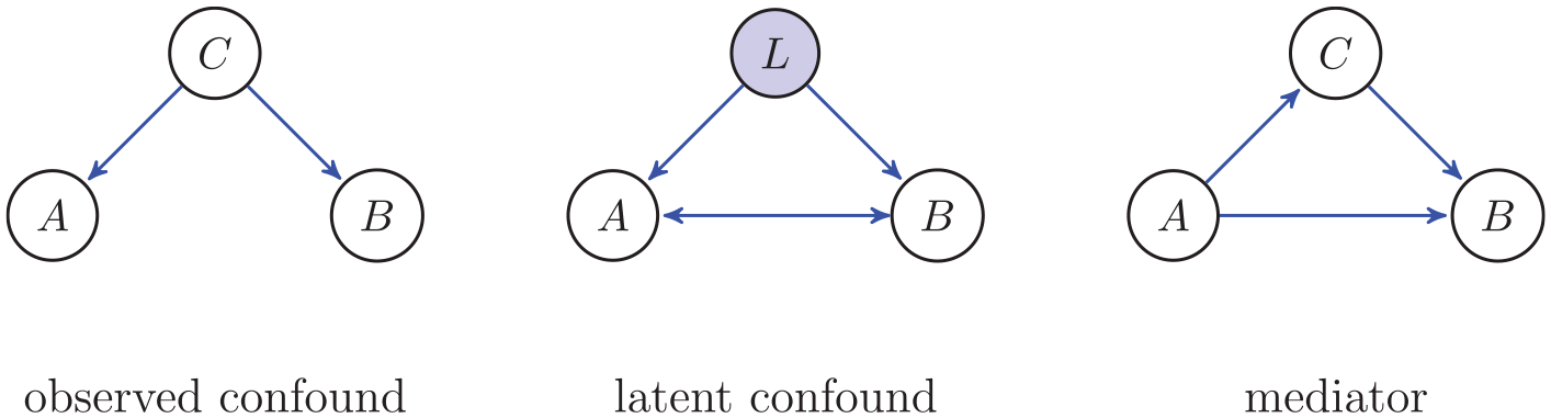
A confound is a common cause situation and can be an observed (left) or an unobserved (latent, middle panel) variable with edges into both A, the putative cause, and B, the putative effect. In the situation of a latent confound the variable L is not observed; often we denote an unobserved confound by A ↔ B. The right panel shows a mediator, where there are two directed paths from A to B; C is not a confound but a mediator for the path A→ C → B.

Figure 2.

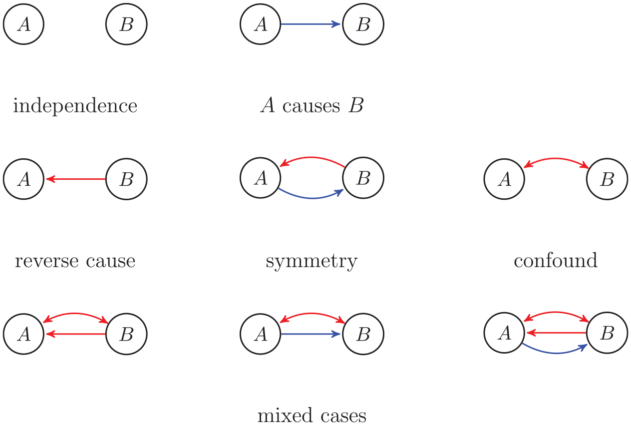
Causal inference of A → B requires excluding six possible alternatives (red edges). Reverse causation A ← B and symmetry A B are excluded because A comes before B; A ↔ B is excluded because it is assumed there are no confounds; the mixed cases are by consequence also excluded. If we then find a statistical dependence between A and B, we can conclude that A → B. Based on Mooij et al. (2020).

A configuration that is similar to a confound but not identical is mediation. The mediator in Figure 1 shows there are two directed paths from A to B; one direct path A → B and one indirect path A → C → B (e.g., Baron & Kenny, 1986). This is clearly different from a confound, since a change in C will lead to a change in B but not to a change in A. A mediator complies with intervening on A and expecting a change in the distribution of B; only now this change in B can both be due to the direct and indirect path. In mediation analysis the intention is to disentangle the direct and indirect effect; this is often quite difficult (Pearl et al., 2016).

We now have the assumptions in place to obtain the causal inference A → B. Consider the possible graphs for the two nodes A and B in Figure 2. We see that incorrect inference could be obtained from a confound or reverse causation (or any of the mixed cases). If we assume that A comes before B, then we can exclude any inference with reverse causation A ← B in Figure 2. If, additionally, A and B are not confounded, then we can exclude any inference with confounds A ↔ B in Figure 2. Then we are left only with the first two possibilities: A B (statistically independent) and A → B. And so, if we find that A and B are statistically dependent, then we infer that A → B. In summary, the reasoning to obtain causal inference is as follows:

There is a statistical dependence between A and B.

A precedes B (no reverse causation).

There is no confounding between A and B.

Hence, A is a cause of B.

In other words, no-confounding, temporal precedence, and statistical dependence together are equivalent to our interventionist account of cause (see Theorem E.1 in Appendix E [available online] and the fifth section). This is quite remarkable since it implies that to obtain causal information in terms of the interventionist account, we do not necessarily have to intervene (Pearl, 2009a; Pearl & Mackenzie, 2018; Spirtes et al., 1993). It also shows that we need to realise that causal claims made by experimental and observational data rely on the exact same set of criteria (see Corollary E.2 in Appendix E). And so, any causal claim, whether in an experimental or observational setting, needs to be evaluated by the strength of its arguments of excluding confounds. Such a causal claim must be supported by other arguments than statistical arguments, both in the experimental (with intervention) and in the observational (without intervention) setting. We shall discuss how confounds are excluded both in the experimental and in the observational setting.

Experimental data: Control and randomisation

The premises 1–3 in the reasoning in the previous section imply that if we can exclude confounds and we know that A comes before B, then statistical dependence is sufficient to claim a causal relation A → B (see e.g., Mooij et al., 2020, Proposition 10; Spirtes et al., 1993, Chap. 9). Hence, in an experiment we need to be certain that A comes before B and that there are no confounds. Then statistical dependence (e.g., a difference between groups or a correlation) establishes A → B.

As to the temporal precedence of A, in an experiment the cause is determined by an intervention, so that for intervention I we get I → A → B. For instance, the type of psychotherapy selected for a patient is an intervention (I), and this determines the psychotherapy for a patient (A), which in turn leads to changes in the symptoms of a disorder (B). In an experiment the intervention necessarily comes before the effect, and so the change in A comes before the change in B. Therefore, we only have to deal with excluding possible confounds.

Experimentation, actually intervening, reduces the difficulty of excluding confounds. There are many different versions of an experiment, but generally, two ingredients are generic: control and randomisation (Cox & Reid, 2000; Howson & Urbach, 2006). Control refers to the concept that an intervention on A is only on A and on no other variables, so that we have I → A and only this edge from I to A. It cannot be the case that, if A is the putative cause of B, then the intervention is a direct cause of both A and B (i.e., A ← I → B, where I is the intervention), because the intervention itself is then a confound. We say that the experiment is controlled if the intervention only determines A and there is no common cause of the intervention I and A, that is, there cannot be any C such that C ← I → A, and there cannot be any L such that I ← L → A (Spirtes et al., 1993, Chap. 9). Intuitively, in a controlled experiment there can be no other causes of A than the intervention. Since a confound implies that both the putative cause and the putative effect are caused by another variable C (see Figure 1), control prevents the presence of any confound, observed or unobserved. So, if there are no other causes of A except the intervention, then there can be no confounds at all. Hence, in a controlled experiment confounders are excluded.

We give an example to illustrate control. Consider the true graph in Figure 3 (top row), where A is not a cause of B but a latent confound L causes both A and B. In an experiment on A, the intervention I → A removes the edge L → A (Figure 3 experiment on A) because there is control over (the distribution of) A. It is then said that the incoming edges to A (the putative cause) are broken (Pearl, 2009a; Pearl et al., 2016; Spirtes et al., 1993). The reason that the edge into A, the putative cause, is removed is because if A is controlled, then there can be no other cause of A; and so, in the graph the edge from L into A is removed. Then, L is no longer a confound because it is not a common cause of A and B in the experiment on A. As a result of the experiment on A, we therefore detect correctly (right column in Figure 3) that there is no causal relation from A to B. If there actually is a causal effect from A to B, then Figure 3 (bottom row) shows that an experiment on A also leads to the correct conclusion in this case of a cause from A to B. So, because there is control in an experiment through the intervention, possible (latent) confounds are removed and correct causal conclusions are obtained.

Figure 3.

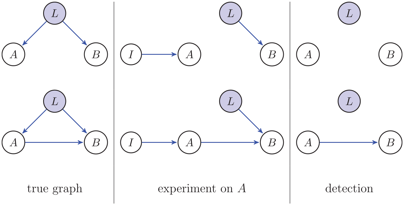
Left are two unknown true graphs including two observed variables A and B and one unobserved latent variable L. The middle panel shows two experiments on A now including the intervention variable I. In the right panel is what can be detected from these experiments on A given that the variable L is not observed.

Randomisation refers to the idea of breaking all possible and often unknown causes of A, the putative cause of B, by means of random assignment to two or more groups (Fisher, 1935, Section II.10). The simplest version is with two groups, an experimental and a control (placebo) group. As with control, we assume in randomisation that there is no common cause between assignment I and putative cause A. Then random assignment to either of the two groups achieves that, in the long run, characteristics of individuals (in psychology and the social sciences) are distributed evenly among the two groups, and this implies that there are no systematic differences between groups (Howson & Urbach, 2006, Chap. 7). In other words, randomisation is a convenient version of obtaining control by breaking possible causes to putative cause A of effect B.

Including a control group serves another purpose that may strengthen the causal claim that A causes B. Referring to the idea of Mill (1843), leaving only one aspect different between the two groups, the only putative cause of B is A. For instance, when investigating a new psychotherapy, comparison to treatment as usual is preferable to no therapy at all, because the treatment as usual resembles the new psychotherapy in many more respects than no therapy at all. And so, there are fewer differences that could also be the cause of B.

Overall, control is the basic ingredient of experimental data; control ensures that no confounds are possible because the putative cause A can have no other causes but the intervention (Howson & Urbach, 2006). In practice, control of the putative cause A is difficult because there are many possible confounders, many of them unknown (and so, latent confounders). And if possible confounders are unknown, it is by definition impossible to take them into account to obtain control. Randomisation is a practical tool that achieves control to a good approximation (in the long run). It works because randomisation breaks confounds from causing A, and so the confounds are nullified (they may still cause B, but not A). But even with randomisation, there is no guarantee. We will consider several examples that show that randomisation may not be sufficient.

Howson and Urbach (2006, Chap. 6) discuss the issue that there might be a possibility for a confound to coincide with the experimental condition. For instance, consider an experiment with random assignment to either the new psychotherapy group or the treatment as usual. But the new psychotherapy is provided by one psychotherapist and the treatment as usual by another psychotherapist. The characteristics of this psychotherapist are such that, on average, the patients obtain fewer symptoms after treatment, fewer also than the group with treatment as usual. In this case, the psychotherapist coincides exactly with the random assignment. And so, the differences between groups are that there is a different psychotherapy, but also a different psychotherapist. Because the psychotherapist coincides exactly with assignment, it is a confound between the intervention (random assignment) and therapy, such that random assignment to treatment does not disconnect the confound (psychotherapist) from the cause (see also Spirtes et al., 1993, Chap. 9, for an excellent example).

Another counter example to randomisation nullifying confounds is that if there are many (denumerable) confounds, and each has a small probability of being unequally represented in the two groups, then all confounds together will have a large probability of obtaining unequal groups in several respects (Deaton & Cartwright, 2018; Howson & Urbach, 2006, Chap. 6). This issue comes from the fact that randomisation is an ideal; it hinges on the concept of probability defined by the frequency interpretation. This implies that, for finite samples, but especially small samples, randomisation may not lead to approximately equal representation of all confounds in the two groups. And so, in general, there is no guarantee that all confounds are nullified.

In order to account for the possible confounders that remain (since an ideal experiment is not attainable), different strategies have been invented (for an excellent list, see Imbens & Rubin, 2015). Propensity scores, stratified analysis, regression adjustment, and parent adjustment are all special cases of what is sometimes called the back-door criterion. An example of a back door is seen in Figure 3 (top left), where the putative cause A is connected to the putative effect B by confound L. If L could be measured, then the back door can be nullified by conditioning on subsets of L, and checking for each value of L the dependence between A and B. If there is no dependence in any of the values of L between A and B, then the correct inference obtains that A does not cause B here (Pearl, 2000; see also Rohrer, 2018 for a discussion on how to cope with this central problem of observational data).

As a final drawback, consider the fact that in an experiment we cannot always differentiate between a common cause and a mediator. Consider again the graph in Figure 3, the bottom row, where the latent variable L (unmeasured) is a confound and there is a direct effect of A → B. In the experiment on A, the intervention I → A breaks incoming edges to A and we may conclude correctly that A causes B. Suppose now that we change the A ← L to A → L, so that A → L → B, and there is a direct effect of A → B. In an experiment on A, outgoing edges from A are not removed, because control only refers to how A (the putative cause) is caused by other variables and not how A may cause other variables. As a consequence, for the experiment on A, the detection of A → B (finding statistical dependence between A and B) is exactly the same either when the causal structure is a common cause, where L causes both A and B (Figure 3, bottom row), or when the causal structure is mediation. In both the common cause and mediator cases, where L is unmeasured, we obtain A as a cause of B. In other words, surprisingly, sometimes in an experiment where an intervention is implemented, a common cause cannot be distinguished from a mediator (Spirtes et al., 1993, Chap. 9).

In all, experimentation (intervention) is a good way to deal with confounds in a generic way; it is a practical and workable way to obtain control. Additionally, the intervention is necessarily before the effect, and hence the cause comes before the effect. So, a causal claim is reduced to determining statistical dependence. This is similar to what we saw in the second section to obtain correct causal inference A → B. However, there are no guarantees with experimentation, even with randomisation.

Observational data: Causal discovery

In observational data, the causal inference is more involved. This is mainly because we cannot easily guarantee that there are no confounds. In the two-variable case discussed in the second section, it is indeed hard to determine the causal direction between A and B (but see Mooij et al., 2016, where nonlinearity is used to detect directionality). But when more than two variables are measured, it becomes possible to determine directionality given certain assumptions. We focus initially on the question of how it is even possible to get causal direction, even when we assume that there are no confounders (causal sufficiency). Subsequently, we will address the problem of discovering causal direction in the presence of latent confounders. We first start with the important concept of d-separation.

In the second section, we discussed the causal Markov and causal faithfulness assumptions, which together make it possible to go from the world of graphs to the world of probability distributions and back. The world of probability distributions applies (un)conditional independence relations between variables: A and B are conditionally independent given C. Such probabilistic statements have to correspond to what we see in the graph, if there is to be a sensible mapping between the world of graphs and the world of probabilities. The analogous concept to conditional independence used in graphs is d-separation, and is about paths between nodes that can be blocked and nodes are then said to be separated. For example, in the graph A → C → B, A and B are d-separated by C; sometimes it is said that C blocks the information from A to B (Pearl, 2000). d-separation is a graphical concept that allows one to determine from the graph which paths are “active” or “inactive.” A path between A and B is a sequence of alternating nodes and edges (in any direction); for instance, A → U → ··· ← B is a path between A and B. A path is active if information can move from A to B; for example A → C → B is active. But A → C ← B is inactive. This is because on the path A → C ← B the node C is a collider node, where two arrows meet head to head and A and B are blocked. For a more precise definition of d-separation, see Appendix B and, for example, Lauritzen (1996), Pearl (2009b, Chap. 1), and Spirtes et al. (1993, Chap. 3).

The concept of d-separation in a graph corresponds to the concept of conditional independence in the probability distribution (obtained from the data). For the graph A → C → B the causal Markov assumption implies that A is conditionally independent of B given C. And conversely, the causal faithfulness assumption goes in the other direction: if A and B are conditionally independent given C, we conclude that A → C → B, A ← C ← B, or A ← C → B.

Although we would like to identify each unique representation of a causal graph with any set of conditional independencies, this is unfortunately not possible. We can only identify from the conditional independencies a set of causal graphs, where only some of the causal directions are identified. Such sets of equivalent graphs are called Markov equivalence sets (see, e.g., Pearl, 2000; Spirtes et al., 1993). Consider Figure 4, both the common cause and the chain. Suppose that we find that A is conditionally independent of B given C and A and B are dependent when not conditioning. Then, we identify with this set of conditional independencies three possible causal graphs: A ← C → B (common cause), A → C → B (chain), and A ← C ← B (chain), because in each case we see that C d-separates A and B and this corresponds to A and B being conditionally independent given C, and A and B are dependent when not conditioning. Hence, in general, the correspondence between graphs and probability distributions is not one to one; there are multiple graphs that correspond to the same set of conditional independence relations.

Figure 4.

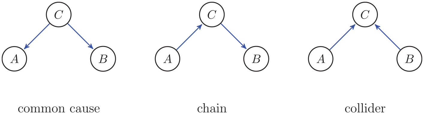
The configurations common cause and chain (a chain could also be the other way around A ← C ← B) have exactly the same conditional independencies (A and B are dependent and A and B are conditionally independent given C). Hence, they are indistinguishable given only data (but including more variables could improve distinguishability). The collider at C has different conditional independencies (A and B are independent but A and B are conditionally dependent given C).

However, there is a specific configuration of edges such that from conditional independencies, a unique graph is implied. This holds for the collider graph in Figure 4. The causal Markov condition implies a very specific set of conditional independence relations for the collider in Figure 4: A and B are conditionally dependent given C, but A and B are independent unconditionally. This is an especially interesting situation. Why do we obtain conditional dependence in this situation where A → C ← B? Suppose that C is the case where someone fails a test, and A is that the failure obtains because of lack of sleep, and B is that the failure obtains because of few hours of study. Then if we know someone failed the test and studied hard, then the cause of failure must be lack of sleep (we have supposed here there are no other causes of failing the test; see Pearl et al., 2016, Chap. 2 for other excellent examples). The unique graph that corresponds to these conditional independencies is the collider in Figure 4. Because of the unique mapping between the d-separations for the collider in Figure 4 and the conditional independencies, we obtain that the directions can be interpreted as causes (given the three assumptions; Spirtes et al., 1993, Chap. 5, Theorem 3.4). Therefore, in observational data, colliders make it possible to obtain the claim that A → B and not the other way around (Pearl et al., 2016). This will be illustrated in the next subsection.

PC algorithm: Assuming no confounders

One of the first implementations of causal discovery is the PC algorithm (the acronym comes from the names of the inventors Peter Spirtes and Clark Glymour). It has been shown that the PC algorithm obtains the correct graph (up to Markov equivalence; Kalisch & Bühlmann, 2007; Spirtes et al., 2000). In the PC algorithm, we assume the causal Markov assumption (d-separation implies conditional independence, Assumption A.1), the faithfulness assumption (conditional independence implies d-separation, Assumption A.2), causal sufficiency (there are no unmeasured confounders, Assumption A.3), there can be no cycles (i.e., feedback, A → ··· → A is not allowed), and there is no selection bias. Especially, the causal sufficiency assumption is too strong to be taken seriously in practice. That is why other algorithms exist that can account for unmeasured confounders. We discuss such algorithms in the next subsection. Also, the assumption that no cycles are allowed is strong and not always realistic. This assumption is, upon some alterations in the concept of d-separation, not necessary so that cycles are allowed (Mooij et al., 2020; Park et al., 2024). The FCI algorithm discussed in the next subsection is an algorithm where cycles can be detected (Mooij & Claassen, 2020).

The PC algorithm considers many different unconditional and conditional independencies (correlations and partial correlations for multivariate normal data) and infers edges from them to construct a causal graph. The algorithm uses all three assumptions explicitly. The data (estimated probability distribution) is used to determine unconditional and conditional independencies to conclude whether or not an edge should be present (using the faithfulness assumption). If for two nodes no unconditional or conditional independence is obtained in the data (i.e., the two nodes are dependent), then an edge between those two nodes obtains (Markov assumption). The interpretation of an edge A → B in the end result of the algorithm is interpreted as a cause (because of causal sufficiency).

In Appendix C, we give an example graph to illustrate why it is possible (given the three assumptions) to obtain causal directions from the PC algorithm; all steps of the PC algorithm for the example graph are described in Appendix C. For the general case, a full description of the algorithm can be found in Spirtes et al. (1993, Section 5.4.2) and Pearl (2000, Section 2.6).

FCI algorithm: Assuming possible latent confounders

The real problem is, of course, that in observational data, there could be many unmeasured (latent) confounders. The essential part of any causal analysis is then to guarantee that any causal inference is not due to unmeasured confounders. In an experimental setup, as we have shown, unmeasured confounders are (approximately) eliminated by randomisation. But in observational data, there is no randomisation process that can break the relation from the confounder to the putative cause. Hence, other steps must be taken to ensure that correct causal inference obtains.

One of the possible solutions to the problem of possible confounders and latent variables is to (1) find evidence for the possibility of confounding and (2) limit causal claims to possible chains of the form A → L → ··· → B, to suggest that A causes B through unmeasured latent variables like L. This is implemented in fast causal inference (FCI; Spirtes et al., 1993). We illustrate this with an example graph. This example is elaborately discussed in Appendix D; here we give a brief description. Extensive descriptions of the FCI algorithm more generally can be found in Spirtes et al. (1993, Chap. 6) and Spirtes et al. (1996), and it has been shown that FCI is correct (Spirtes et al., 2000) and has good finite sample properties (Raghu et al., 2018; Temme, 2006).

We consider how FCI encodes evidence for confounders in the output graph. In the FCI output in Figure 5, the bidirected edge B ↔ D indicates that there is evidence of a confounder, and so we cannot make a causal claim. The small circles in the FCI output graph indicate that FCI cannot determine whether there should be an arrow (→) or an endpoint (−). Because this represents uncertainty, we indicate edges where there could possibly be a confound also with a bidirected edge ↔. (The graph is then not maximally informative, but we are interested here in conservative estimates of causal claims.)

Figure 5.

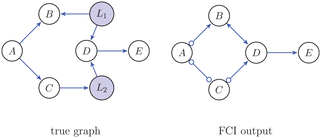
The true graph with latent confounder L₁ and mediator L₂. The output of the FCI algorithm without the latent variables (marginal), where ○ means that FCI cannot determine which mark it should be, and where the bidirected edge ↔ means that there is evidence for a latent confound.

We start with (1) determining that there is evidence for confounding. The reason FCI can differentiate between a possible confounder and no confounder between B and D is the following: Intuitively, if we find for two nodes that cannot be d-separated and for each there is no directed path from one to the other, then there might be a confound (see Spirtes et al., 1993, Section 6.7, for a detailed account; Zhang, 2008). We consider this for the example graph in Figure 5 for the latent confound L₁ on B and D. We first show that it appears to be the case that B ← D, and then we show that it appears to be the case that B → D; both cannot be simultaneously true and so we conclude that there is a collider. Conditioning on C in the true graph in Figure 5 makes A and D conditionally independent. But conditioning on B and C together will render A and D conditionally dependent. This suggests there must be some collider at B. This collider appears to come from D because conditioning on A in the true graph in Figure 5 makes B and C independent; so there is no edge C → B. There is also no edge E → B because conditioning on D makes B and E conditionally independent. Since there are no other variables to cause the collider at B, it seems as if B ← D. Furthermore, there is also a collider at D and this appears to come from B. This is because B and C are conditionally dependent given A and D. So, there seems to be an edge B ← D and an edge B → D, which cannot simultaneously be true. As a result, there is a latent confounder B ← L₁ → D. In the FCI output in Figure 5 we therefore see a bidirected edge between B and D, indicating that there is a possible confound.

As for (2), it is also possible that there are unmeasured variables, like the mediator L₂ in the true graph of Figure 5, that form a chain, here C → L₂ → D. Then C is still a cause of D because if we change C for this causal chain C → L₂ → D, the probability distribution of D will change accordingly. Because such unmeasured variables are not excluded, any causal inference with respect to the measured variables must allow for the possibility that there are such unmeasured variables like L₂ that are part of a chain from C to D in Figure 5.

Taken together, we see that for this graph it is quite difficult to obtain causal claims. If there are latent confounders, then FCI will obtain a bidirected edge representing a possible latent confounder (Zhang, 2008). Such conservative decisions for causal claims are warranted because we are trying to obtain information about interventions while not having performed any.

Causal evidence and experimental or observational data

The question here is not whether experimental or observational data is superior to obtain causal evidence; there certainly are some advantages for causal claims on the basis of experimental data (but see Deaton & Cartwright, 2018). The question here is whether both experimental and observational data are subject to the same criteria. The answer to this latter question is a resounding yes. Any causal claim either from experimental or observational data is subject to the same criteria.

The criteria for causal evidence are 1–3 in the second section, which we repeat here for convenience (Mill, 1843, Book III, Chap. XII; see also Mooij et al., 2020, Definition B.2):

There is a statistical dependence between A and B.

A precedes B (no reverse causation).

There is no confounding between A and B.

We show in Theorem E.1 (in Appendix E) that this definition of causal evidence is equivalent to the definition we have been using (Definition B.3; in Appendix B): A causes B if, whenever we change A, then a change in the probability distribution of B is obtained (given the causal Markov assumption A.1 and the faithfulness assumption A.2; in Appendix A). This equivalence is a remarkable fact, for we can apply the three criteria to observational (or quasi-experimental) data and make causal claims in terms of interventions (Illari & Russo, 2014; Pearl & Mackenzie, 2018). Causal claims are important because we often want to say what happens when we intervene; we are interested mostly in prediction upon intervention (Carnap, 1966). One of the most permeating examples in psychology is that of therapy: Will the intervention of therapy lead to fewer symptoms in a patient? Experimental evidence is not always available and so it may be informative to use causal claims from observational data (e.g., data obtained from patients on a waiting list) or from quasi-experimental evidence (Imbens & Rubin, 2015). But as we have seen, there are limitations.

The three criteria of causal evidence can be traced back to both experimental and observational data. In experimental data, we have seen that the intervention comes before the effect (criterion 2), and control (e.g., randomisation) prevents confounders (criterion 3; see the second and third sections). Then, to determine a causal relation only requires a statistical dependence. In observational data, we have seen that directionality (criterion 2) is obtained as a result of the unique correspondence between the collider structure A → C ← B and that A and B are conditionally dependent given C (see the fourth section). In such cases, upon finding that A and B are conditionally dependent given C and A and B are independent when not conditioning on C, we can conclude that A → C ← B. Furthermore, confounding cannot in general be excluded (criterion 3), as in the case of the ideal experiment, but evidence for confounders resulted in the conclusion that, in some cases, no causal claim could be made. The final graph obtained from observational data includes both causal and noncausal connections between variables. In this way, the uncertainty about a causal claim is represented clearly in the result.

Randomisation in experiments clearly has several advantages. As mentioned, in (the idealisation of) an experiment, randomisation eliminates all possible (latent) confounds. This is an extremely powerful and convenient technique to obtain control of the putative cause. Additionally, randomisation allows for creating appropriate confidence intervals and testing the null hypothesis (Cox & Reid, 2000, Chap. 2). Randomisation also allows for the possibility of performing blind and double-blind studies; such procedures reduce observer bias (Spirtes et al., 1993). These advantages certainly make experiments an attractive method to obtain causal claims.

With observational data, on the other hand, confounds are very difficult to ascertain. But we showed that it is possible with observational data with multiple variables to classify pairs of variables as likely to be causal or unlikely to be causal (using FCI).

However, there are also cases where we are able to distinguish causal structures with observational data that we cannot distinguish with experimental data. We saw an example in the third section, where we were unable to distinguish between a confound and mediator case with an intervention (cf. Figure 3). We show in Appendix F that, using observational data, we can distinguish between a confound and a mediator.

In summary, it turns out that the most important characteristic for causal claims is to be able to exclude confounds. In the experimental setting, this is achieved by control. Control in an experimental setting implies that the putative cause is fully determined by the intervention, and so there cannot be a latent confound (i.e., no variable L such that A ← L → B). In practice, control can be achieved by randomisation (with some limitations). And in observational data, we cannot exclude all confounds and so we search for evidence of possible confounders, and indicate this in the result if there is such evidence. Additionally, if it is possible that latent mediators are present, then any causal claim is actually, possibly, an indirect cause (causal chain).

Empirical illustration

Here we illustrate how the ideas about causal modelling can be applied to a theory about eating disorders. From the theory about eating disorders, we can build causal models that make predictions about conditional independence relations (using the Markov assumption) that are testable in data. This is a good strategy to test specific hypotheses about causal relations between variables in general, where the assumptions to obtain causal inference are made clear (e.g., Dawid, 2003; Pearl et al., 2016). Additionally, having theoretical models and testing them will lead to information about where to intervene, as we illustrate below.

Eating disorders are highly prevalent mental disorders that involve distorted body image and food-related cognitions and behaviours (American Psychiatric Association, 2013) and that have a great impact on the health and quality of life of affected individuals and their loved ones (Dakanalis et al., 2017). It is, however, still necessary to examine how exactly the various symptoms (e.g., weight and shape concerns, binge eating, restraint) are related. Insight into the exact mechanistic relationships between these various elements of eating disorder symptoms would be critical to select the best starting point for interventions. Another aspect that is relevant is the high comorbidity of eating disorders with internalising disorders such as anxiety and depression (Vervaet et al., 2021). Yet, it is unclear whether these internalising symptoms can be best seen as a cause or as a consequence of eating disorder problems or that both types of symptoms are elicited by a third factor (e.g., low meaning in life). Again, for selecting the most promising starting point for interventions, it would be critical to have insight in the mechanistic relationships between eating disorder symptoms and symptoms of comorbid internalising disorders.

Ignoring the factors that promote the comorbidity of internalising symptoms and symptoms of eating disorders might be one of the aspects limiting treatment success leading to higher mortality rates than the general population (van Hoeken & Hoek, 2020). Clearly, a better understanding of the mechanisms at play in eating disorder symptoms and their comorbidity is warranted.

Because causal information is about prediction, a causal graph can help both with understanding eating disorders and with obtaining information on how to best intervene (predict). A causal graph suggests ways of disorder development and maintenance. For instance, when considering the prominent example of the transdiagnostic eating disorder symptom model by Fairburn et al. (2003), knowing that overvaluation of weight, shape, and eating and their control have an effect on dietary restraint, which in turn affects binge eating, could suggest that increased overvaluation may lead to subsequent disordered eating behaviour. Such understanding can also be used in determining how to intervene. Applying the FCI might be a helpful strategy to elucidate the mechanistic relationships between the various eating disorder symptoms as well as the mechanisms involved in the prevalent comorbidity of eating disorder symptoms and symptoms of internalising disorders.

To illustrate ideas of causal modelling, we provide three different theoretical accounts of the causal relations between the most relevant variables for the models of eating disorders. The most relevant variables are: (a) symptoms of eating disorder, like dietary restraint, binge eating, and compensatory behaviour, together denoted by S; (b) overvaluation of eating, weight, and shape and their control, denoted by O; (c) depressive symptoms, denoted by D; (d) ineffectiveness, denoted by I; and finally, (e) presence of meaning in life, denoted by M. When considering the nodes most relevant to comorbidity within the study of eating disorders, three possibilities about causal relationships between them seem feasible (see Figure 6):

(a) Meaning M in life as an endpoint: Eating disorder symptoms S and overevaluation O have a causal effect on depression symptoms D, leading then to a decrease in perceived ineffectiveness I and meaning in life M.

(b) Meaning in life M as a mediator: Overvaluation of eating, weight, and shape O together with the other eating disorder symptoms S lead to a decreased perceived ineffectiveness I as well as low meaning in life, which then in turn lead to heightened depression symptoms D.

(c) Meaning in life M as a cause for comorbidity: Low meaning in life M causes perceived ineffectiveness I which then has a causal effect on eating disorder symptoms S as well as on depression symptoms D.

We shall discuss elaborately the first account (a) of the theoretical concepts implemented in a graph (set of hypotheses); we discuss the implications of the theoretical causal relationships to testable conditional independencies. The other two accounts (b) and (c) are discussed only briefly, as the implications can be similarly derived.

Figure 6.

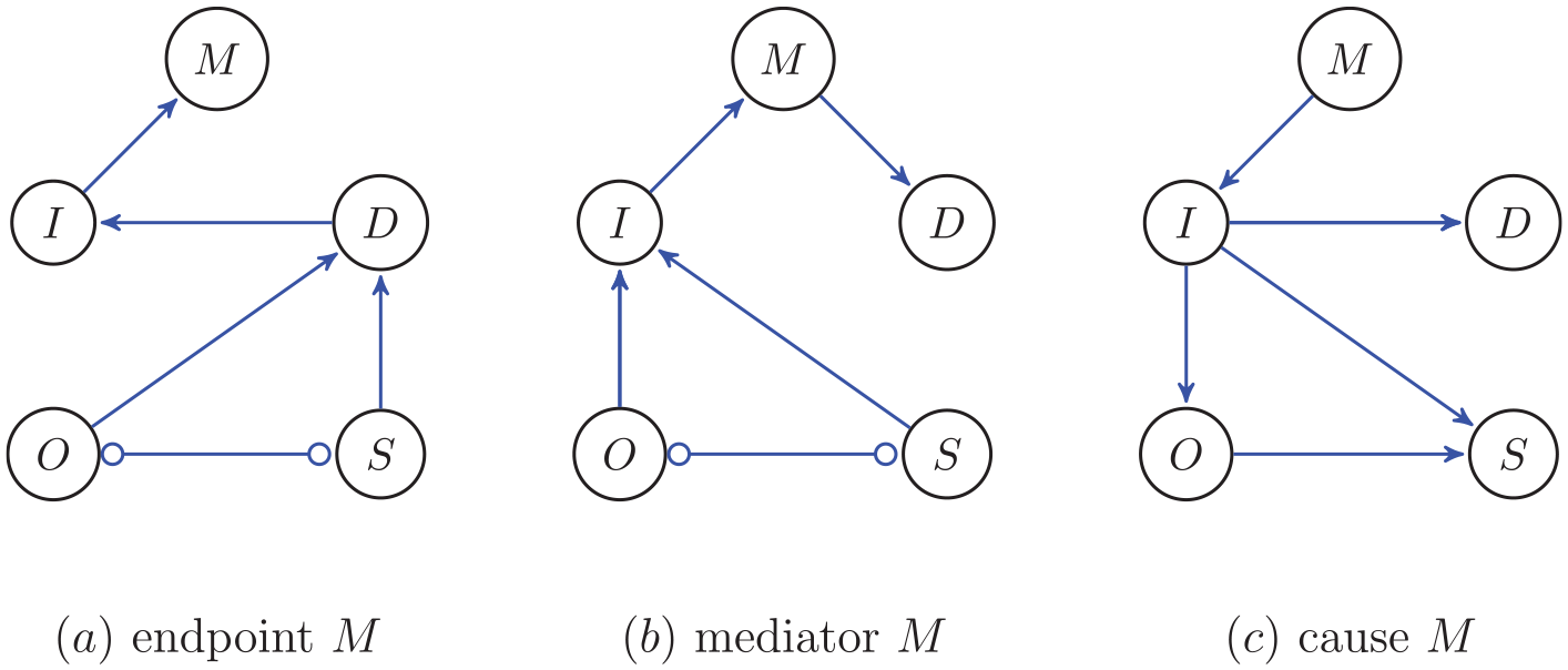
Three possible configurations for the most relevant variables of eating disorders. The edge ○−○ between O and S represents that the endpoints at O and S cannot be identified by FCI; there might be a confound.

In the first account of eating disorders, shown in the left panel of Figure 6, meaning in life M is an effect variable (end of a chain). In this account, depression D is caused by overvaluation O and symptoms S. Furthermore, depression D causes ineffectiveness I and in turn, ineffectiveness I causes low meaning in life M. This is a theoretical account, meaning that each edge (and absence of an edge) is derived from theory. And from these causal relations we can derive predictions about what, according to this causal graph, we should find in the data (using d-separation and the causal Markov assumption, see the fourth section). The predictions about conditional independencies are as follows. We start with connectivity without direction and then discuss directions. O and S should be conditionally independent of I and M given D; in other words, D screens off O and S from I and M. In the FCI algorithm (see the fourth section), the hypothesis is tested whether O and S on the one hand and I and M on the other hand are conditionally independent given D. If this is correct, then indeed, we may conclude that there are no edges from O and S to I and M that do not go through D (all edges from O and S to I and M must go through D). In a similar vein, I screens off D from M, and so if this were correct, FCI should obtain conditional independence between D and M given I. Furthermore, if there is an edge in the graph, then there is no set of other variables that can make the dependence between the two nodes disappear. For instance, the edge I → M implies that given any subset of the remaining variables, I and M are dependent. This holds for all the edges in the graph.

The directions can be obtained whenever there are colliders (see the fourth section). For instance, there is a collider O → D ← S. This collider induces a particular (different) dependence between O and S when conditioned on D than when not conditioned on D; this makes it possible for FCI to determine that there is a collider. FCI will not be able to obtain all directions from the conditional independencies. The heuristic is that if there is no collider at either end of the edge, then switching direction will not lead to a different conditional independence relation, and hence, it will not lead to a different d-separation.

The edge O ○−○ S has a ○ at O and S to indicate that FCI cannot identify whether there should be an arrowhead or not; there could be a confound.

The second account of eating disorders (b) in terms of the relevant variables is the mediator M (middle panel of Figure 6). The main difference with the first account (a), effect M (left panel of Figure 6), is that now I screens off O and S from D and M.

The third account of eating disorders (c) in terms of the relevant variables is the common cause M (right panel of Figure 6). Here, the effects are basically reversed; M is the common cause of D, O, and S and I causes D, O, and S, but I and M are not connected.

These are the theoretical predictions of the three models. Using theory to guide the construction of a causal graph leads to the possibility of distinguishing between them because of the implications for conditional independence relations (and the Markov and faithfulness assumptions, see the second section). We can now apply the FCI algorithm to a dataset to determine for which one of the above models there is most evidence, or for which set of edges there is evidence.

We will focus on a dataset used in a recent network study by Schutzeichel et al. (2024), which examined the role of meaning-related factors, such as feelings of ineffectiveness, presence of meaning in life, and the basic psychological needs of autonomy, competence, and relatedness in eating disorders and comorbid internalizing symptomatology. One-time questionnaire data was collected from the general population (n = 501) from Dutch-, German-, and English-speaking participants above the age of 16. Maximum age was 75 (with a mean of 30.5 years) and BMI ranged from 16.6 to 54.9 (with a mean of 24.11). 22.1% of the sample was within a clinically relevant cut-off score of 2.5 on the Eating Disorder Examination-Questionnaire (EDE-Q; Fairburn & Beglin, 2008; Rø et al., 2015). The authors not only made use of classic undirected network analysis based on correlational data, but they also applied the FCI algorithm with α = 0.1 to the data by means of the pcalg package in R (R code for causal discovery algorithms; Kalisch & Bühlmann, 2014). After using predictive mean matching and 50 iterations to deal with missing data, the FCI network was plotted using igraph (Csardi & Nepusz, 2006). To ensure stability of the edges, 500 subsamples using 80% of the total sample size were created and only edges that were present in at least 75% of all 500 subsamples remained in the graph. R-code of these analyses is available online (see Schutzeichel et al., 2024).

In this dataset, there are more variables than we discussed above for the three accounts of eating disorders. We deliberately reduced the number of variables for the hypothesised graphs to be able to clearly describe all implications for the data. The variables meaning in life M, ineffectiveness I, overvaluation O, and depression D are the same, but in the real dataset, we have for the symptoms S the following three variables: dietary restraint R, binge eating B, and compensatory behaviour C. All variable names are in the caption of Figure 7 (see Schutzeichel et al., 2024, for more details).

Figure 7.

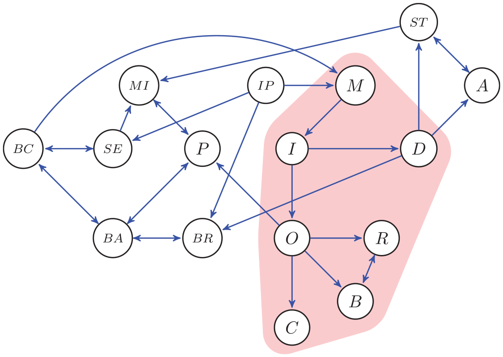
Graph of the FCI output for the data on eating disorders. The variables are: meaning in life M, ineffectiveness I, overevaluation O, depression D, dietary restraint R, binge eating B, compensatory behaviour C, interpersonal problems IP, mood intolerance MI, self-esteem SE, perfectionism P, basic need of competence BC, basic need of autonomy BA, basic need of relatedness BR, Anxiety A, and stress ST. The shaded area represents the nodes used for the hypotheses about the causal relations (a)–(c) in Figure 6, except that S there is here C, B, and R.

As shown in Figure 7, results demonstrated that, in line with Fairburn et al.’s (2003) transdiagnostic theory, overvaluation of weight, shape, and eating O influenced eating disorder symptoms, such as restraint R, binge eating B, and the intention to compensate for caloric intake C. While the original theory describes an interaction between these symptoms, the causal graph was unable to determine direction of causality between restraint R and binge eating B and showed otherwise no connection between these variables.

The investigation of meaning-related factors displayed a clear causal pathway from interpersonal problems IP (which is part of the transdiagnostic model) to meaning in life M, to ineffectiveness I, which then had a causal effect on overvaluation O, as well as depressive symptoms D. Note that this is in line with the proposed possibility (c), see also Figure 6. Following the latter pathway, depressive symptoms D exhibited influence on both anxiety A and stress ST. However, the algorithm could not clearly distinguish whether stress ST mediated the relationship with anxiety A, or if both depressive symptoms D and anxiety A contributed to the experience of stress ST; there might also be a confound.

Despite insufficient information or latent (i.e., unmeasured) variables in this dataset, the FCI function nevertheless provided relevant insights into the mechanisms of an eating disorder symptom network. This knowledge could now further be used to develop preventative measures for those struggling with eating disorder symptoms such as weight and shape concerns by targeting meaning in life M and ineffectiveness I directly to break the progression towards eating disorders or internalising disorders or as an add-on to current treatments for patients with eating disorders. In line with the former, a recent intervention directly targeting meaning in life by van Doornik et al. (2024) demonstrated effectiveness in reducing symptoms of eating disorders and internalising comorbidity in undergraduate students.

In conclusion, with this practical example, we can see that applying causal discovery to observational data can contribute valuable information on not only working mechanisms but also possible pre-intervention and intervention options. Adding the subsampling method led to more certainty about the presence of causal relations between nodes in this study, so that any interpretations drawn do not suffer from stability issues of the network. FCI furthermore shows a clear benefit over other causal inference algorithms as it only exposes causal relations when latent confounds can be ruled out. Within this practical example, we can observe this directly by detecting both correlational and causal output in the form of bidirectional and unidirectional arrows, respectively.

Conclusion and discussion

Our aim here was to show that causal claims can be obtained not only from randomised control trials (experiments) but also from observational data, where no intervention has been implemented. We believe that in many cases where experimentation might be difficult or impossible to implement or might not lead to the desired circumstances for an effect to show up (i.e., not ecologically valid), observational data can be used to obtain causal claims. These causal claims are to some extent uncertain, mostly because it is difficult to exclude confounds. However, causal claims from observational data are categorised in terms of evidence for causal claims and no evidence for causal claims. Additionally, applying resampling techniques (here we used subsampling), it is possible to obtain relative certainty about the causal claims.

We have in fact shown here that the common interpretation of causation, the interventionist account (Woodward, 2003), is equivalent to the causal evidence account (the three criteria discussed in the fifth section). This implies that we can interpret causal claims obtained from observational data, where we apply the three criteria, in exactly the same way as we do when we have actually intervened (see Pearl, 2009b; Spirtes et al., 1993). This means that causal claims from observational data can be very useful. We illustrated this with an example dataset on eating disorder symptoms. The causal analysis led to the idea that meaning in life may be relevant to also consider in treatments, as this may be involved in the progression or maintenance of the eating disorder symptoms. Supporting this claim and thereby also showing the predictive validity of the FCI-output, it was indeed shown that an intervention to increase meaning in life in individuals with eating disorder symptoms not only increased meaning in life but also reduced overvaluation of eating, weight, and shape as well as symptoms of depression (van Doornik et al., 2024).

In conclusion, then, experiments are not the only way to obtain causal information; applying carefully the ideas of causal discovery can also lead to causal claims with some degree of certainty. An interesting development is that we can combine information from experiments and observations in a single analysis (e.g., Mooij et al., 2020; Peters et al., 2016; Spirtes et al., 1993, Chap. 9). Such analyses may reveal more than analyses from either experimental or observational data alone.

Supplemental Material

sj-docx-1-tap-10.1177_09593543251325506 – Supplemental material for Causal inference: Principles unifying experimental and observational accounts

Supplemental material, sj-docx-1-tap-10.1177_09593543251325506 for Causal inference: Principles unifying experimental and observational accounts by Lourens Waldorp, Franziska Schutzeichel and Peter J. de Jong in Theory & Psychology

Supplemental Material

sj-docx-2-tap-10.1177_09593543251325506 – Supplemental material for Causal inference: Principles unifying experimental and observational accounts

Supplemental material, sj-docx-2-tap-10.1177_09593543251325506 for Causal inference: Principles unifying experimental and observational accounts by Lourens Waldorp, Franziska Schutzeichel and Peter J. de Jong in Theory & Psychology

Supplemental Material

sj-docx-3-tap-10.1177_09593543251325506 – Supplemental material for Causal inference: Principles unifying experimental and observational accounts

Supplemental material, sj-docx-3-tap-10.1177_09593543251325506 for Causal inference: Principles unifying experimental and observational accounts by Lourens Waldorp, Franziska Schutzeichel and Peter J. de Jong in Theory & Psychology

Supplemental Material

sj-docx-4-tap-10.1177_09593543251325506 – Supplemental material for Causal inference: Principles unifying experimental and observational accounts

Supplemental material, sj-docx-4-tap-10.1177_09593543251325506 for Causal inference: Principles unifying experimental and observational accounts by Lourens Waldorp, Franziska Schutzeichel and Peter J. de Jong in Theory & Psychology

Footnotes

Funding

The authors disclosed receipt of the following financial support for the research, authorship, and/or publication of this article: This work was supported by Gravity project, “New Science of Mental Disorders,” the Dutch Research Council and the Dutch Ministry of Education, Culture and Science (NWO), grant number 024.004.016.

ORCID iDs

Lourens Waldorp

Franziska Schutzeichel

Peter J. de Jong

Supplemental material

Supplemental material for this article is available online.

Author biographies

Lourens Waldorp is associate professor at the Psychological Methods group of the Department of Psychology at the University of Amsterdam. He studied both psychology and mathematics at the University of Amsterdam, and did his PhD in developmental psychology, also at the University of Amsterdam. His expertise is in probability, statistics, networks, causality, and dynamics, with a focus on modelling. He has collaborations with different organisations to model processes (over time) of different kinds of psychopathology. Recent publications include (with J. Kossakowski & H. L. van der Maas) “Perturbation Graphs, Invariant Prediction and Causal Relations in Psychology,” in British Journal of Mathematical and Statistical Psychology (2024) and (with O. Ryan & J. Haslbeck) “Non-Stationarity in Time-Series Analysis: Modeling Stochastic and Deterministic Trends,” in Multivariate Behavioral Research (2025).

Franziska Schutzeichel is a doctoral student at the Department of Clinical Psychology and Experimental Psychopathology at the University of Groningen. Her research focuses on the transdiagnostic role of meaning in life for eating disorder symptoms and comorbid internalising symptoms from a network perspective. Her recent publications include “Life Meaning and Feelings of Ineffectiveness as Transdiagnostic Factors in Eating Disorder and Comorbid Internalizing Symptomatology – A Combined Undirected and Causal Network Approach,” in Behaviour Research and Therapy (2024) and “A Meaning-Centered Intervention for Undergraduate Women with High Weight and Shape Concerns—Replication of a Randomized Controlled Trial,” in European Eating Disorders Review (2025).

Peter J. de Jong is full professor of experimental psychopathology at the University of Groningen. Following a transdiagnostic approach, his research focuses on cognitive-motivational mechanisms that may help explain the aetiology and course of various disorders including eating disorders and depression. Recent publications include (with E. C. Bennik & K. A. Glashouwer) “‘If I Feel Disgusted, I Will Become Fat’: Disgust-Based Emotional Reasoning in the Context of Weight and Shape Concerns,” in Journal of Experimental Psychopathology (2024).

References

American Psychiatric Association. (2013). Diagnostic and statistical manual of mental disorders (5th ed.).

Baron

R. M.

Kenny

D. A.

(1986). The moderator–mediator variable distinction in social psychological research: Conceptual, strategic, and statistical considerations. Journal of Personality and Social Psychology, 51(6), 1173–1182. https://doi.org/10.1037/0022-3514.51.6.1173

Carnap

(1966). An introduction to the philosophy of science. Dover Publications.

Cartwright

(2001). What is wrong with bayes nets? The Monist, 84(2), 242–264. https://www.jstor.org/stable/27903726

Cox

Reid

(2000). The design of experiments. Chapman and Hall.

Csardi

Nepusz

(2006). The igraph software package for complex network research. InterJournal, Complex Systems, 1695(5), 1–9.

Dakanalis

Clerici

Bartoli

Caslini

Crocamo

Riva

Carra

(2017). Risk and maintenance factors for young women’s DSM-5 eating disorders. Archives of Women’s Mental Health, 20(6), 721–731. https://doi.org/10.1007/s00737-017-0761-6

Dawid

(2003). Causal inference using influence diagrams: The problem of partial compliance. In Green

P. J.

Hjort

N. L.

Richardson

(Eds.), Highly structured stochastic systems (Vol. 27, pp. 45–65). Oxford University Press.

Deaton

Cartwright

(2018). Understanding and misunderstanding randomized controlled trials. Social Science & Medicine, 210, 2–21. https://doi.org/10.1016/j.socscimed.2017.12.005

10.

Durrett

(2010). Probability: Theory and examples (2nd ed.). Duxbury Press.

11.

Eberhardt

Scheines

(2007). Interventions and causal inference. Philosophy of Science, 74(5), 981–995. http://www.jstor.org/stable/10.1086/525638

12.

Fairburn

C. G.

Beglin

(2008). Eating disorder examination questionnaire (EDE-Q 6.0). In Fairburn

C. G.

(Ed.), Cognitive behavior therapy and eating disorders (pp. 309–313). Guilford Press.

13.

Fairburn

C. G.

Cooper

Shafran

(2003). Cognitive behaviour therapy for eating disorders: A “transdiagnostic” theory and treatment. Behaviour Research and Therapy, 41(5), 509–528. https://doi.org/10.1016/S0005-7967(02)00088-8

14.

Fisher

(1935). The design of experiments. Haffner Press.

15.

Gillies

(2019). Causality, probability, and medicine. Routledge.

16.

Hausman

D. M.

Woodward

(1999). Independence, invariance and the causal Markov condition. The British Journal for the Philosophy of Science, 50(4), 521–583. https://www.jstor.org/stable/40072257

17.

Howson

Urbach

(2006). Scientific reasoning: The Bayesian approach. Open Court Publishing.

18.

Illari

Russo

(2014). Causality: Philosophical theory meets scientific practice. Oxford University Press.

19.

Imbens

G. W.

Rubin

D. B.

(2015). Causal inference in statistics, social, and biomedical sciences. Cambridge University Press.

20.

Kalisch

Bühlmann

(2007). Estimating high-dimensional directed acyclic graphs with the PC-algorithm. The Journal of Machine Learning Research, 8, 613–636.

21.

Kalisch

Bühlmann

(2014). Causal structure learning and inference: A selective review. Quality Technology & Quantitative Management, 11(1), 3–21. https://doi.org/10.1080/16843703.2014.11673322

22.

Lauritzen

(1996). Graphical models. Oxford University Press.

23.

Lauritzen

(2001). Causal inference from graphical models. In Barndorff Nielsen

O. E.

Cox

D. R.

Kluppelberg

(Eds.), Complex stochastic systems (pp. 63–107). Chapman and Hall / CRC Press.

24.

Mill

J. S.

(1843). A system of logic: Ratiocinative and inductive, being a connected view of the principles of evidence, and the methods of scientific investigation. John W. Parker.

25.

Mooij

J. M.

Claassen

(2020). Constraint-based causal discovery using partial ancestral graphs in the presence of cycles. Proceedings of the 36th Conference on Uncertainty in Artificial Intelligence, 124, 1159–1168.

26.

Mooij

J. M.

Magliacane

Claassen

(2020). Joint causal inference from multiple contexts. Journal of Machine Learning Research, 21, 1–108.

27.

Mooij

J. M.

Peters

Janzing

Zscheischler

Schölkopf

(2016). Distinguishing cause from effect using observational data: Methods and benchmarks. Journal of Machine Learning Research, 17, 1–102.

28.

Park

Waldorp

L. J.

Ryan

(2024). Discovering cyclic causal models in psychological research. Advances in Psychology, 2, Article e72425. https://doi.org/10.56296/aip00012

29.

Pearl

(2000). Causality: Models, reasoning and inference. Cambridge University Press.

30.

Pearl

(2009a). Causal inference in statistics: An overview. Statistics Surveys, 3, 96–146. https://doi.org/10.1214/09-SS057

31.

Pearl

(2009b). Causality: Models, reasoning and inference. Cambridge University Press.

32.

Pearl

Glymour

Jewell

N. P.

(2016). Causal inference in statistics: A primer. John Wiley & Sons.

33.

Pearl

Mackenzie

(2018). The book of why: The new science of cause and effect. Basic Books.

34.

Peters

Bühlmann

Meinshausen

(2016). Causal inference by using invariant prediction: Identification and confidence intervals. Journal of the Royal Statistical Society: Series B. Statistical Methodology, 78(5), 947–1012. https://www.jstor.org/stable/44682904

35.

Peters

Janzing

Schölkopf

(2017). Elements of causal inference: Foundations and learning algorithms. MIT Press.

36.

Raghu

V. K.

Ramsey

J. D.

Morris

Manatakis

D. V.

Sprites

Chrysanthis

P. K.

Glymour

Benos

P. V.

(2018). Comparison of strategies for scalable causal discovery of latent variable models from mixed data. International Journal of Data Science and Analytics, 6, 33–45. https://doi.org/10.1007/s41060-018-0104-3

37.

Reichenbach

(1956). The direction of time: Volume 65. University of California Press.

38.

Rø

Ø.

Reas

D. L.

Stedal

. (2015). Eating disorder examination questionnaire (EDE-Q) in Norwegian adults: Discrimination between female controls and eating disorder patients. European Eating Disorder Review, 23(5), 408–412. https://doi.org/10.1002/erv.2372

39.

Rohrer

J. M.

(2018). Thinking clearly about correlations and causation: Graphical causal models for observational data. Advances in Methods and Practices in Psychological Science, 1(1), 27–42. https://doi.org/10.1177/2515245917745629

40.

Schutzeichel

Waldorp

L. J.

aan het Rot

Glashouwer

K. A.

Frey

M. I.

Wiers

R. W.

de Jong

P. J.

(2024). Life meaning and feelings of ineffectiveness as transdiagnostic factors in eating disorder and comorbid internalizing symptomatology—A combined undirected and causal network approach. Behaviour Research and Therapy, 172, Article 104439. https://doi.org/10.1016/j.brat.2023.104439

41.

Spirtes

(2010). Introduction to causal inference. Journal of Machine Learning Research, 11(5), 1643–1662.

42.

Spirtes

Glymour

Scheines

(1993). Causation, prediction and search. Springer-Verlag.

43.

Spirtes

Glymour

Scheines

(2000). Causation, prediction, and search. MIT Press.

44.

Spirtes

Meek

Richardson

(1996). Causal inference in the presence of latent variables and selection bias. ArXiv. https://arxiv.org/pdf/1302.4983

45.

Temme

(2006). Constraint-based inference algorithms for structural models with latent confounders—Empirical application and simulations. Computational Statistics, 21(1), 151–182. https://doi.org/10.1007/s00180-006-0257-8

46.

van Doornik

S. F. W.

Glashouwer

K. A.

Ostafin

B. D.

de Jong

P. J

. (2024). The effects of a meaning-centered intervention on meaning in life and eating disorder symptoms in undergraduate women with high weight and shape concerns: A randomized controlled trial. Behavior Therapy, 55(1), 177–190. https://doi.org/10.1016/j.beth.2023.05.012

47.

van Hoeken

Hoek

H. W

. (2020). Review of the burden of eating disorders: Mortality, disability, costs, quality of life, and family burden. Current Opinion in Psychiatry, 33(6), 521–527. https://doi.org/10.1097/YCO.0000000000000641

48.

Vervaet

Puttevils

Hoekstra

R. H. A.

Fried

Vanderhasselt

M. A.

(2021). Transdiagnostic vulnerability factors in eating disorders: A network analysis. European Eating Disorders Review, 29(1), 86–100. https://doi.org/10.1002/erv.2805

49.

Williamson

(2005). Bayesian nets and causality. Oxford University Press.

50.

Williamson

(2019). Establishing causal claims in medicine. International Studies in the Philosophy of Science, 32(1), 33–61. https://doi.org/10.1080/02698595.2019.1630927

51.

Woodward

(2003). Making things happen: A theory of causal explanation. Oxford University Press.

52.

Zhang

(2008). On the completeness of orientation rules for causal discovery in the presence of latent confounders and selection bias. Artificial Intelligence, 172(16–17), 1873–1896. https://doi.org/10.1016/j.artint.2008.08.001

Supplementary Material

Please find the following supplemental material available below.

For Open Access articles published under a Creative Commons License, all supplemental material carries the same license as the article it is associated with.

For non-Open Access articles published, all supplemental material carries a non-exclusive license, and permission requests for re-use of supplemental material or any part of supplemental material shall be sent directly to the copyright owner as specified in the copyright notice associated with the article.

0.00 MB

0.03 MB

0.16 MB

0.18 MB

0.09 MB