Sage Journals: Discover world-class research

Abstract

Many manufacturing companies are always looking for a way to reduce energy consumption by utilizing energy-efficient production methods. These methods can be different depending on the type of products and production technology. For instance, one of the ways to increase energy efficiency and keep the precision of production is to use robots for the transportation of the parts among the machines and loading/unloading the machines. This technology is affordable compared to the technologies used in manufacturing companies. Manufacturing companies that rely on robotics technology must have a strategy to reduce energy costs and at the same time increase production by adjusting the intensity of processing or controlling the production rate. This study presents an exact solution method for flexible robotic cells to control the production rate and minimize energy consumption, which aims to both reduce electricity prices and minimize greenhouse gas (GHG) emissions under a lead time of production. Then, considering the NP-hardens nature of the problem, a heuristic solution method based on the genetic algorithm (GA) is proposed. Using the proposed approach, manufacturing companies will be able to make more accurate decisions about processing intensity and process scheduling while ensuring sustainability.

Keywords

Flexible robotic cell sustainability energy-efficient scheduling genetic algorithm

Introduction

Millions of people are already suffering from the devastating effects of extreme climate change disasters. Today, greenhouse gases (GHGs), such as methane, which is formed by agricultural activities similar to animal manure, are at their highest levels compared to previous decades. Additional emissions such as CO₂ are produced from natural processes such as breathing and burning fossil fuels such as coal, oil, and gas.¹ Therefore, one of the important issues for policymakers in different countries is to decide on the cost of measures related to the reduction of GHG emissions. In this regard, they should have the ability to compare the costs of renewable energy sources and sustainable production.^2,3 Sustainable production is the formation of goods and services using pollutant-free procedures and systems, in addition to saving energy and natural resources. The use of sustainable production systems leads to achieving general development strategies, reducing future environmental and social costs, strengthening financial competitiveness, and reducing poverty in societies.^4,5

One of the possible ways to improve the stability of production systems is to use robotic technology and control the amount of electricity consumption,^6,7 aiming to have an energy-efficient manufacturing platform.⁸ Production speed of the robotic and/or fully automated systems can be adjusted when the time of production is limited. If there is such a limitation for changing the robot processing speeds, using a parallel-machine system is the traditional answer.⁹ On the other hand, enabling to change the robots’ processing speeds, whether manual or using a sensor,¹⁰ are directly caused different amounts of electricity consumption. Using this technology is one of the useful solutions for controlling electricity costs.^11,12

Within either manufacturing companies or transportation and logistics systems, performing tasks take place using utility energy sources (e.g., electric current or natural gas).^13,14 Specifically, manufacturing processes such as machining and assembly require the use of energy-consuming tools. Most production systems, such as flowshop systems, work in multiple shifts and have limited production flexibility.^15,16 For sustainable development, it is necessary for manufacturing companies to reduce their energy consumption, because excessive energy consumption has a destructive effect on the environment. For example, the emission of GHGs, acidification of the environment, and extensive land use are among the disadvantages of this excessive use. On the other hand, energy is a vital element of production. This is why energy demand reduction is limited in scope and dependent on the desired output. Therefore, increasing the ratio of energy input to the desired outcome in a production process, i.e. increasing energy efficiency, is an essential part of sustainable production.⁸

To our knowledge, no research has been conducted to establish energy-efficient production planning and control in flexible robotic cells (FRCs) under time limitations for production. Recently, Wang et al.¹⁷ proposed a solution method to paint large objects using robots for a service organization. In FRCs, each machine should perform all the activities associated with a part that needs distinct operations and processing times. When a robot loads a part into a machine, the machine can perform several more processes before transferring the product to the storage system. The only processing intensity that may be addressed in FMC for energy-efficient scheduling is the speed of machine and robot processes. As a fact, manufacturing companies prefer to run their machines at ultimate production speed to satisfy the customer demands according to the lead time, however, working at high speed will affect the electricity used by machines.¹⁸

Considering the complexity and limitations of production using FMC, as well as the difficulty of accurate modeling and optimization to achieve a reduction of energy consumption in modern production systems, the study presents a mathematical model and metaheuristic solution method for this problem. Hence, the aim of this article is to focus on the problem of energy-efficient scheduling of FRCs with a robot to pick and place parts, CNC machines to perform processes, and buffers to store raw materials and products. CNC machines and robots can work at different speeds. This research aims to achieve optimal energy consumption for FRCs while meeting demand considering the lead time, by setting appropriate speed levels for the machines and finding the best time sequence of operations.

The related literature is reviewed in the next chapter, and the problem is defined and formulated in the third chapter. In Chapter 4, the metaheuristic-based solution method is proposed and explained in detail, and the initial parameters are set to utilize the algorithm. Chapter 5 contains the detail of the case study, the related results after solving the problem by the proposed algorithm, and discussions about the results. Finally, the study is concluded in the last chapter.

Literature review

The global manufacturing industry is highly fragmented, and a large portion of it is dedicated to small- and medium-sized businesses. Deterioration of the environment and rising energy costs put a lot of pressure on the manufacturing industry to save energy and reduce GHG emissions. Companies should consider energy efficiency planning based on energy consumption rates to increase their energy efficiency. An imbalance in energy consumption and more use causes an increase in the energy tariff rate and leads to a significant increase in these costs. To address this, a pricing scheme is used to encourage customers to reduce energy consumption, thereby balancing energy demand. The energy consumption of each job varies during the production process, which means that operations that require a large amount of energy must be scheduled over months while operations that require a small amount of electricity can be used continuously.¹⁹

Particularly energy-intensive industrial processes are of special relevance when it comes to production planning and scheduling using uniform machines that are processing parts under some restrictions.²⁰ Here, a significant amount of energy is required to power the machines, which are tasked with the task of converting input (i.e., raw materials) to the desired output (i.e., final products). Giret et al.²¹ investigated sustainable scheduling in a broader sense, emphasizing solution techniques in multiobjective situations. Cui et al.²² discussed the scheduling of power loads in demand response programs but do not go into detail about scheduling. Garwood et al.²³ conducted a review of works that include energy considerations in production settings using simulation. Narciso and Martins²⁴ organized the latest machine learning developments into energy-related scheduling applications. Bänsch et al.²⁵ conducted a survey of the literature on energy-related research in manufacturing settings, with a particular emphasis on mathematical optimization-based decision support models. Recently, Zhang et al.²⁶ proposed an optimization algorithm using a deep-learning method to solve the life-cycle production scheduling problem considering real-time cycles.

Mouzon and Yildirim²⁷ are pioneers in incorporating energy usage into production scheduling. Energy-efficient scheduling promotes energy efficiency primarily in two ways: by reducing energy consumption and by lowering energy costs. The previous research on energy-efficient scheduling is mostly concerned with reducing energy consumption at various stages, such as the processing stage, the setup stage, and the standby stage. Recently, energy-efficient scheduling has been shown to reduce energy costs when both energy usage and energy prices are included. Energy-related planning including energy-efficient planning, low-carbon planning, and sustainable planning in diverse manufacturing environments has been increasingly considered in the literature.²⁸

Research on reducing environmental impacts of manufacturing companies is mainly focused on minimizing transportations in supply chains using ground or aerial logistics,^29,30 or it is limited to production scheduling of a single-machine cell, parallel/unparalleled machine in flow shop type production, and/or job shop manufacturing. For the energy-efficient scheduling of single-machine cells, Fang et al.³¹ discussed the scheduling of a single-machine problem, aiming to minimize the total electricity expenditure. Later, Cheng et al.³² developed a bi-objective mixed-integer linear programming model to minimize the total electricity cost and the makespan of a single-machine batch processing problem. To solve large-size problems efficiently, they developed a heuristic-based e-constraint method. Tan et al.³³ scrutinized the economic load dispatch, aiming to minimize electricity charges with penalties caused by jumps among adjacent slabs. Zhao et al.¹² considered campaign decisions and managing demands to address manufacturing scheduling problems in the rolling sector for producing steel. They dealt with a multistage production and proposed a mixed-integer nonlinear programming model to solve the problem.

For hot-rolled batch processing, Hu et al.,³⁴ developed a model aiming to minimize the entire penalty caused by the alterations in width, thickness, and hardness among adjacent slabs, in addition to the electricity costs. Wang et al.³⁵ considered a flow shop with two machines and studied the related permutation scheduling problem to optimize the overall electricity price of processing tasks. Geng et al.³ developed a multiobjective ant lion optimization method to solve a scheduling problem related to a hybrid re-entrant flow shop aiming to minimize the total process time and minimize the energy consumption charge, simultaneously. Ho et al.³⁶ considered the joint optimization of the total producing time and electric charge in a flow shop with two machines. They studied the economic issues of the optimum solution of a scheduling problem considering the permutations of jobs, aiming to minimize the electricity charge without increasing the total process time.

From the parallel/unparalleled machines, Ding et al.³⁷ studied the scheduling problem include of unrelated parallel-machine. Their objective was to minimize the overall electricity consumption cost when there is a deadline for handling all the jobs in the considered manufacturing system. Cheng et al.³⁸ established an MILP formulation to solve a parallel machine scheduling problem, aiming to minimize the total electricity charges. Zang et al.³⁹ proposed a continuous-time MILP model to solve a two-stage parallel machine production floor include of identical speed-scaling machines at the first step and unrelated parallel machines at the next step.

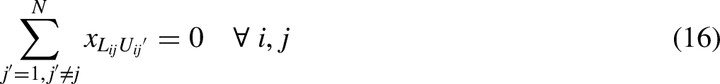
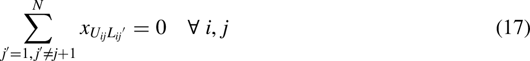
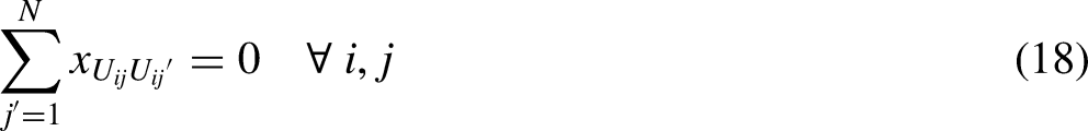
During the past years, the authors have studied various types of FRC scheduling problems and their applications in real cases in industries. For instance, in 2018, Nejad et al.⁴⁰ considered an FRC to produce identical parts cyclically, including identical CNC machines, and separate input, and output buffers, aiming to find a sequence of operations to minimize the cycle time (Figure 1 illustrates the scheme of the mentioned FRC). To solve such a problem they developed a mathematical model and discussed the lower bound for the total makespan.⁴¹

Figure 1.

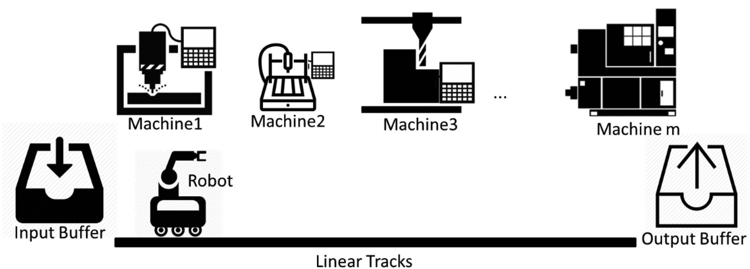
m-machine flexible robotic cell.

Then, they proved and considered the NP-hardness of such a problem and developed an SA approach for solving the problem in cases of having a high number of CNC machines in the production line.⁴² Later on, a bi-objective scheduling problem for the FRCs has been considered to minimize the cost of the cyclic production and the cycle time, simultaneously.⁴³ They developed a genetic algorithm (GA) to solve such a problem and utilized the Taguchi method to set the initial parameters of the algorithm. Afterward, they considered a real-life sequencing problem of FRC with individual input buffers for each CNC machine and proposed a GA, SA, and a hybrid metaheuristic algorithm based on GA and SA.⁴⁴

Numerous studies have been conducted on energy efficiency scheduling in a variety of generic manufacturing systems. Numerous scholars have examined simple production systems, such as single machines and parallel machines.⁴⁵ However, few studies have been conducted on complex manufacturing systems such as flow shops, flexible flow shops, job shops, and flexible job shops.² As far as the authors’ knowledge in this context, no report on the energy efficiency scheduling of FRCs has been made, especially considering the time limits to produce the products. Considering the importance of FRC in industries and the complexity of such problems, the authors decided to focus on the batch production type of FRCs in this study, aiming to minimize the developed energy cost function for running such a system using exact and heuristic solution methods.

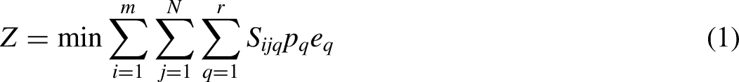
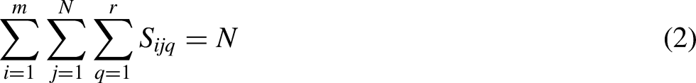
Problem definition and formulation

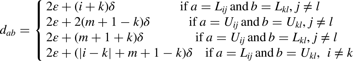
To solve the robot movements scheduling problem, by minimizing the energy consumption of the robot and machines to produce identical parts, the definitions, parameters, and variables are as follows:

$L_{i j}$ : Loading of machine i for the timecap $j^{t h}$ time

$U_{i j}$ : Unloading of machine i for the $j^{t h}$ time

$A$ : Set of loading and unloading tasks

$q$ : Diverse machines’ speed levels, from 1 to r

$S_{i j q}$ : 1; if the machine i is loaded for the $j^{t h}$ time with speed level q, otherwise; 0

$p_{q}$ : The processing time of a machine if it operates with a speed level $q$

$e_{q}$ : Energy consumption of a machine if it operates with speed level q, per time unit

$m$ : Number of machines

$N$ : Total demand, which is the number of required parts to be produced by the system

$M_{i}$ : The number of parts to be produced by machine $i$

$x_{a b}$ : 1; if task b is done immediately after task a, otherwise; 0

$t_{a b}$ : Completion time of task b if it is done immediately after task a, otherwise; 0

T: Acceptable time threshold of production

$ε$ : Time of loading/unloading a machine when the robot stands by the machine

$δ$ : Travel time of the robot between two consecutive machine

$d_{a b}$ : The robot transportation time for performing task b immediately after task a, which is not related to the machines’ process times, can be calculated using the following formula where $i, j, k, a n d l$ are indices of machines.

d_{a b} = {\begin{matrix} 2 ε + (i + k) δ if a = L_{i j} and b = L_{k l}, j \neq l \\ 2 ε + 2 (m + 1 - k) δ if a = U_{i j} and b = U_{k l}, j \neq l \\ 2 ε + (m + 1 + k) δ if a = U_{i j} and b = L_{k l}, j \neq l \\ 2 ε + (| i - k | + m + 1 - k) δ if a = L_{i j} and b = U_{k l}, i \neq k \end{matrix}

Mathematical formula:

Z = min \sum_{i = 1}^{m} \sum_{j = 1}^{N} \sum_{q = 1}^{r} S_{i j q} p_{q} e_{q}

(1)

Subject to:

\sum_{i = 1}^{m} \sum_{j = 1}^{N} \sum_{q = 1}^{r} S_{i j q} = N

(2)

\sum_{j = 1}^{N} \sum_{a} x_{L_{i j} a} = M_{i} \forall i; a \neq L_{i j}

(3)

\sum_{q = 1}^{r} S_{i j q} \geq \sum_{q = 1}^{r} S_{i j + 1 q} \forall i, j

(4)

\sum_{q = 1}^{r} S_{i j q} = \sum_{a} x_{L_{i j} a} \forall i, j; a \neq L_{i j}

(5)

\sum_{q = 1}^{r} S_{11 q} = 1

(6)

\sum_{a} x_{a b} \leq 1 \forall a, b; a \neq b

(7)

\sum_{a} x_{L_{i j} a} = \sum_{b} x_{b U_{i j}} \forall i, j; a \neq L_{i j}; b \neq U_{i j}

(8)

t_{L_{11} U_{11}} \geq (\sum_{q = 1}^{r} S_{11 q} p_{q} + d_{L_{11} U_{11}}) x_{L_{11} U_{11}} + (2 ε + δ)

(9)

t_{L_{11} L_{i 1}} \geq d_{L_{11} L_{i 1}} x_{L_{11} L_{i 1}} + (2 ε + δ) d o e s \forall i; i \neq 1

(10)

t_{L_{i j} L_{i^{'} j^{'}}} \geq (\sum_{a} t_{a L_{i j}} + d_{L_{i j} L_{i^{'} j^{'}}}) x_{L_{i j} L_{i^{'} j^{'}}} \forall i, j, i^{'}, j^{'}; a \neq L_{i j}; a \neq L_{i^{'} j^{'}}; i j \neq i^{'} j^{'}

(11)

t_{L_{i j} U_{i^{'} j^{'}}} \geq x_{L_{i j} U_{i^{'} j^{'}}} \times M a x {\begin{matrix} \sum_{a} t_{a L_{i j}} + d_{L_{i j} U_{i^{'} j^{'}}} \\ \sum_{b} t_{b L_{i^{'} j^{'}}} + \sum_{q = 1}^{r} S_{i^{'} j^{'} q} p_{q} + (m + 1 - i^{'}) δ + 2 ε \end{matrix}} \forall i, j, i^{'}, j^{'}; a, b \neq L_{i j}; a, b \neq U_{i^{'} j^{'}}

(12)

t_{U_{i j} L_{i^{'} j^{'}}} \geq x_{U_{i j} L_{i^{'} j^{'}}} (\sum_{a} t_{a U_{i j}} + d_{U_{i j} L_{i^{'} j^{'}}}) \forall i, j, i^{'}, j^{'}; a \neq L_{i^{'} j^{'}}; a \neq U_{i j}; i j \neq i^{'} j^{'}

(13)

\begin{aligned} t_{U_{i j} U_{i^{'} j^{'}}} \geq x_{U_{i j} U_{i^{'} j^{'}}} \times M a x {\begin{matrix} \sum_{a} t_{a U_{i j}} + d_{U_{i j} U_{i^{'} j^{'}}} \\ \sum_{b} t_{b L_{i^{'} j^{'}}} + \sum_{q = 1}^{r} S_{i^{'} j^{'} q} p_{q} + (m + 1 - i^{'}) δ + 2 ε \end{matrix}} \\ \forall i, j, i^{'}, j^{'}; a, b \neq U_{i j}; a, b \neq U_{i^{'} j^{'}}; i j \neq i^{'} j^{'}; i j \neq i j^{'} \end{aligned}

(14)

\sum_{j^{'} = 1}^{N} x_{L_{i j} L_{i j}^{'}} = 0 \forall i, j

(15)

\sum_{j^{'} = 1, j^{'} \neq j}^{N} x_{L_{i j} U_{i j}^{'}} = 0 \forall i, j

(16)

\sum_{j^{'} = 1, j^{'} \neq j + 1}^{N} x_{U_{i j} L_{i j}^{'}} = 0 \forall i, j

(17)

\sum_{j^{'} = 1}^{N} x_{U_{i j} U_{i j}^{'}} = 0 \forall i, j

(18)

t_{a b} \leq M x_{a b} \forall a, b \in A; a \neq b

(19)

t_{a b} \leq T \forall a, b \in A; a \neq b

(20)

x_{a b} \in {0, 1} \forall a, b

(21)

t_{a b} \geq 0 \forall a, b

(22)

S_{i j q} \in {0, 1} \forall i, j, q

(23)

N \geq M_{i} \geq 0 \forall i

(24)

The first equation is the objective function, which indicates that the total energy consumption must be minimized. Equation (2) guarantees that all demand is satisfied, and consequently. Equation (3) finds the amount of total production by each machine and equation (4), shows the sequence of jobs on a particular machine. Equation (5) makes sure that one speed is selected for any loaded task, and Equation (6) ensures that machine 1 is the first machine to be loaded in the production period. Equations (7) and (8) ensure that there exists one and only one activity immediately after a loading activity, and for each loading activity of each machine, there must be an unloading activity for the same machine. The completion time of each task is calculated by Equations (9) to (14). Equations (15) to (18) respectively guarantee that a machine cannot be loaded again before its previous job is unloaded, a machine cannot be unloaded again if its previous job has not been unloaded, and a machine can be loaded just after its previous job is unloaded, and two consecutive unloading activities cannot be performed on a machine. Equation (19) ensures that the completion time of any performed activity can be a positive value; zero otherwise. Equation (20) ensures that the time limit of the production period is given and fixed, and finally, Equations (21) to (24) define the positive and binary variables.

According to the literature, the traditional TSP is a nondeterministic polynomial-time hardness problem, which is called NP-hard in short.⁴⁶ Therefore, those problems that include TSP, like vehicle routing and transportation scheduling, have been proven to be NP-hard type problems. Accordingly, it has been reported that more than 800,000 s (more than 223 h) is needed to solve a simple FRC problem containing just six machines in the cell with a fixed amount of time for producing identical parts and there is no report mentioning solving such problems containing more than that number of machines.⁴¹ Hence, it is clear that the considered problem in this research belongs to NP-hard type problems. Different types of solution approaches have been developed to solve such problems. Metaheuristic methods are one of the most powerful approaches that search for finding the optimal solution in a feasible area in a short time and with high efficiency. Consequently, in this research, a GA has been proposed to solve the problem, as the GA is one of the most well-known metaheuristic algorithms for solving different types of NP-hard problems in the literature.⁴⁷

The developed GA

The GA starts by generating a set of random initial solutions. After computing the fitness function values of these solutions, the algorithm tries to improve the solution by using some distinguished operators such as crossover and mutation.^48,49 The detail of the developed GA in this research are the followings:

Encoding

A solution is presented by an array including 2n + m elements in which n is the number of parts to be produced, and m is the number of machines. The following assumptions must be considered to generate numbers for the first 2n elements:

An integer number from 1 to 2m is allowed to be generated.

An integer belonging to the interval of $[1, m]$ indicates the loading of the first m machines correspondingly, and an integer belonging to the interval of [m + 1, 2m] indicates their, respectively.

For each number generated in the interval of $[1, m]$ , like g, there must be a number in the interval of [m + 1, 2m], like h, in a way that h = g + m. Similarly, for each number generated in the interval of [m + 1, 2m], like h’, there must be a number in the interval of [1, m] before it, like g′, in a way that g′ = h′−m.

The last m elements indicate the speed level of the corresponding CNC machine which processes the parts with that speed level. Let us consider the representation of a random solution for a three-machine FRC, shown in Figure 2, in which five parts are going to be produced with the machines. In this case, the related chromosome contains

2 * 5 + 3 = 13

cells. The first-left 10 elements are related to loading and unloading the machines. For instance, the first, second, fourth, and seventh elements correspond to loading machine 1, loading machine 3, unloading machine 1, and unloading machine 3, respectively. Therefore, the figure shows

L_{1} L_{3} L_{2} U_{1} U_{2} L_{1} U_{3} L_{2} U_{1} U_{2}

activity order. The last three elements illustrate that machine 1, machine 2, and machine 3 are processing the parts with speed levels of 1, 2, and 1, respectively.

Figure 2.

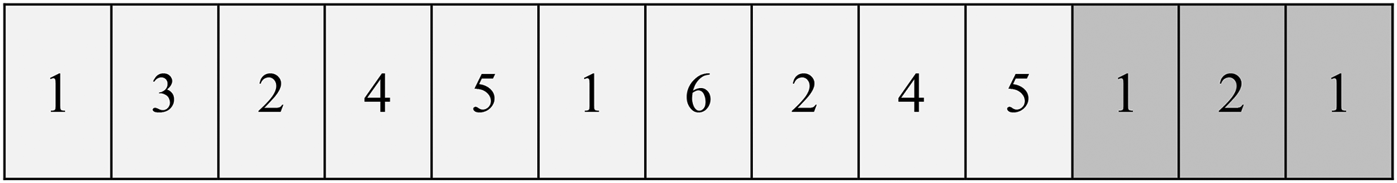
Representation of a solution for a 3-machine FRC. FRC: flexible robotic cell.

Initial solution

The GA starts with generating a population of random solutions. To make solutions feasible, there is a repair function that ensures that all loading activities have been unloaded and that this unloading activity is after the loading.

Evolution

The population evolves through crossover and mutation operations. Binary crossover is incorporated for the crossover operation. For mutation operation, three operations are considered and only one of them is applied on a chromosome randomly with equal probability; Swap, Reversion, and Insertion.⁵⁰ In the swap operation, one pair of genes is selected and their positions in the chromosome are swapped. In reversion operation, two genes of the chromosome are selected and the order of the genes between these selected genes is reversed. The insertion operator selects a gene and inserts it into a new random position.

It is obvious that each selected operation is performed independently on the first and second parts of the chromosomes, related to the sequence of the jobs and speed levels of the machines. Furthermore, it is mandatory to repair the genes after crossover and mutation operations. It should be mentioned that the repair function should not limit the randomness of the solutions. The unbalanced genes are selected randomly pair by pair and the values are changed in a way to fix the problem. In Figure 3, the pseudo-code of the proposed GA in this study is represented. Additionally, Figure 4 demonstrates the flowchart of the proposed GA.

Figure 3.

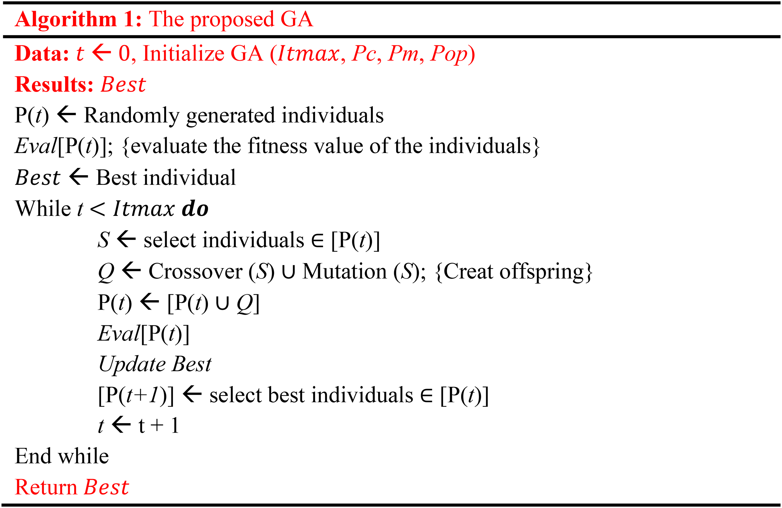
The pseudo-code of the proposed GA. GA: genetic algorithm.

Figure 4.

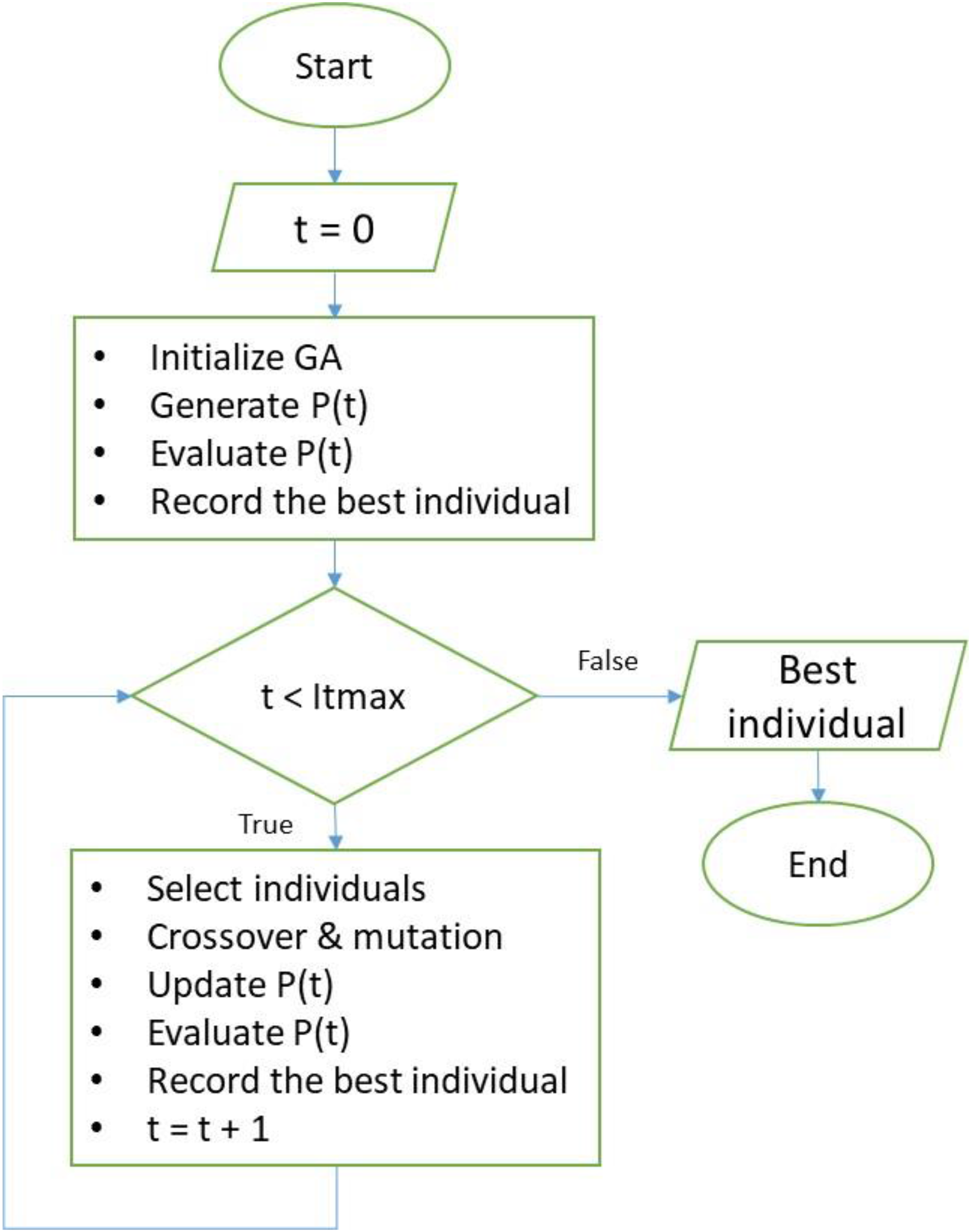
The flowchart of the proposed GA. GA: genetic algorithm.

Completion time and energy consumption calculations for a given solution

There are two steps for calculating the completion time of a given solution. The first step is calculating the duration times of loading, unloading, and transporting the parts by the robot among the machines and buffers. The second step is computing robot waiting times when the robot is ready to unload the part from a machine but the machine is still processing the part.

Let us consider a three-machine cell (its general form has been shown in Figure 1), where $ε = 1$ , $δ = 2$ , the order is like $L_{1} L_{3} L_{2} U_{1} U_{2} L_{1} U_{3} L_{2} U_{1} U_{2}$ , and machines 1 and 3 are processing the parts with speed level 1, in which $P_{1} = 180$ seconds and machine 2 is processing the parts by speed level 2, in which $P_{2} = 300$ seconds. The times needed for performing the robot operations in the first step are calculated by using the d_ab formula given in the problem definition and formulation section, plus the time for loading the first machine at the beginning which is $ε + δ + ε = 4$ . For example, $d_{L_{1} L_{3}}$ is $2 ε + 4 δ = 10$ . Similarly, times between $L_{3} L_{2}$ , $L_{2} U_{1}$ , $U_{1} U_{2}$ , $U_{2} L_{1}$ , $L_{1} U_{3}$ , $U_{3} L_{2}$ , $L_{2} U_{1}$ , and $U_{1} U_{2}$ are calculated as 12, 10, 10, 12, 8, 14, 10, and 10, respectively, which is 96 s in total.

The robot may wait before performing each unloading activity, and these waiting times are not trivial to compute. Let $w_{1}$ to $w_{5}$ be the waiting times before performing the first to the last unloading activities according to the mentioned order, where some or even all of them might be zero. The updated times between the completion of the successive activities in the given order are 4 for $L_{1}$ , 10 for $L_{1} L_{3}$ , 12 for $L_{3} L_{2}$ , $10 + w_{1}$ for $L_{2} U_{1}$ , $10 + w_{2}$ for $U_{1} U_{2}$ ,12 for $U_{2} L_{1}$ , $8 + w_{3}$ for $L_{1} U_{3}$ , 14 for $U_{3} L_{2}$ , $10 + w_{4}$ for $L_{2} U_{1}$ , and $10 + w_{5}$ for $U_{1} U_{2}$ . Thus, the completion time for this order is $C T = 4 + 10 + 12 + (10 + w_{1}) + (10 + w_{2}) + 12 + (8 + w_{3}) + 14 + (10 + w_{4}) + (10 + w_{5}) = 100 + w_{1} + w_{2} + w_{3} + w_{4} + w_{5} .$ The time between the completion of $L_{i}$ and $U_{i}$ must be at least $(2 ε + (m + 1 - i) δ) + p_{1}$ for machine i. Hence, the total time between the completion of $L_{1}$ to $U_{1}$ is $10 + 12 + 10 + w_{1} = 32 + w_{1}$ . This time should be at least $(2 + (3 + 1 - 1) 2) + 180 = 188$ . Therefore $w_{1} \geq 156$ .

Considering a similar procedure to find the other waiting times, the following inequalities are obtained.

w_{1} + w_{2} + w_{3} \geq 132

w_{1} + w_{2} \geq 286

w_{3} + w_{4} \geq 156

w_{4} + w_{5} \geq 286

Consequently, the completion time for the given order is

C T = 100 + w_{1} + w_{2} + w_{3} + w_{4} + w_{5}

, which should be minimized to find the minimum values for the waiting times. This can be done by solving the linear programming model with the objective function of

M i n C T = 100 + w_{1} + w_{2} + w_{3} + w_{4} + w_{5}

, subject to the five obtained inequalities.

To calculate the total energy consumption of the mentioned example, energy consumption by the machines and the robot should be considered. Since in this example, machine 1 and machine 3 are processing with speed level 1, and they produce three parts, they are using $3 * 180 * E_{1}$ energy units in total, and the consumption of machine 2 with speed level 2 to produce two parts is $2 * 300 * E_{2}$ . The energy consumption of the robot is its working time multiplied by its consumption which is $100 * E_{R}$ . Therefore, the total energy consumption for producing all five parts is $3 * 180 * E_{1} + 2 * 300 * E_{2} + 100 * E_{R}$ .

Considering the energy consumption for the faster and slower speed levels as 9.1 and 3.3 watts per minute, respectively, and energy consumption of 0.7 watts per minute, for robot movements, the total energy consumption for producing the parts with the faster level is 137.67 watts. Solving this problem with the same parameters value as the presented exact method, where three parts are processed using the faster speed level, and the other two parts are processed with the slower speed level, gives the total energy consumption of 116.07 watts. The calculations show that the proposed method has the potential to improve total energy consumption by up to 15.69%, which is found by $\frac{137.67 - 116.07}{137.67} * 100 % .$

Results and discussions

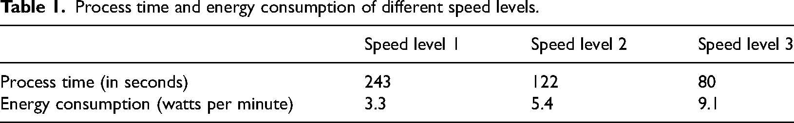
A real-case problem with a demand of 50 has been considered to be performed by the FRC, similar to what is shown in Figure 1. Seven CNC machines are working in parallel and have been located in a line layout at the same distance from each other. These machines are able to process the parts at three different speed levels, say 1, 2, and 3, in which the first speed level is the slowest, the second is medium, and the third/last is the fastest one. Each of the speed levels incurs special energy consumption and process time. Expectedly, the speed level and energy consumption have negative relation; i.e. the lowest speed level causes a lower energy consumption, the second one has a medium energy consumption, and the highest speed level causes a higher energy consumption. Table 1 contains process times and energy consumption of the different speed levels in terms of seconds and watts per minute, respectively.

Table 1.

Process time and energy consumption of different speed levels.

	Speed level 1	Speed level 2	Speed level 3
Process time (in seconds)	243	122	80
Energy consumption (watts per minute)	3.3	5.4	9.1

The robot is responsible for transporting the parts among buffers and machines, loading, and unloading the machines with an energy consumption of 0.7 in terms of watts per minute. It takes an unprocessed part from the input buffer, at the beginning of the production line, and loads one of the machines according to the previously dictated schedule. Additionally, the robot unloads a finished part from a machine and put the part in the output buffer, which is located at the end of the line right after the last machine. The transportation time of the robot between every two machines or between a buffer and its closest machine is 2 s, and the time of loading or unloading of each part by the robot is 1 s. Three steps have been considered to deal with the considered problem as follows:

Step 1: According to the provided pseudocode and flowchart of the developed GA in this study, in the first step the number of iterations, number of populations, crossover percentage, and mutation percentage must be decided. In this study, the algorithm was set to 500 iterations, a population of 100, crossover, and mutation percentages of 70 and 60, respectively. The problems have been solved by an Intel^® Core^™ i5-3320M CPU@2.60 GHz, and 4 GB Ram on a Windows 10 Operating System. Firstly, the problem was solved without considering a time limit for processing all 50 parts in three different situations as follows:

All the machines are processing the parts with the first speed level only (243 s),

All the machines are processing the parts with the second speed level only (122 s),

All the machines are processing the parts with the third speed level only (80 s),

The energy consumption for these problems was 689.15, 569.91, and 627.57, and the total process time for them was 4893, 4544, and 3412, respectively.

Step 2: In the second step, the machines were free to be set at any speed level, to find the minimum energy consumption. In this case, the optimal energy consumption was 569.81 (watts/minute), with a total time of 4134 (seconds), and CPU time of 3121.93 s.

Step 3: Different time limits have been considered for the problem in this step. The time limits are started from a feasible level, which means reaching a value that there is no feasible solution for the problem even when all the machines work at their highest speed level. For this reason, after some trials, 2100 s were found. This means that the considered problem does not have any feasible solution considering a time limit of less than 2100 for sure. In other words, when the time limit is 2100 s, the total process time violates the time limitation. Then, the time limit is increased up to the level that all machines can process the parts with their minimum speed as mentioned in Step 2. Table 2 provides the obtained results of solving the mentioned problem considering different time limits.

Table 2.

Results with different time limits for processing of 50 parts.

Test no.	Process time levels (s)	Energy consumption levels (watts/minute)	Time limit (s)	Total time (s)	Energy consumption (watts/minute)	CPU time (s)
1	243/122/80	3.3/5.4/9.1	2200	2198	628.41	2677.37
2	243/122/80	3.3/5.4/9.1	2300	2282	608.43	3141.14
3	243/122/80	3.3/5.4/9.1	2400	2398	606.31	2754.93
4	243/122/80	3.3/5.4/9.1	2500	2492	578.41	2679.64
5	243/122/80	3.3/5.4/9.1	2600	2598	581.08	3151.09
6	243/122/80	3.3/5.4/9.1	2700	2694	597.32	2527.88
7	243/122/80	3.3/5.4/9.1	2800	2764	587.77	2958.74
8	243/122/80	3.3/5.4/9.1	2900	2880	573.15	2369.19
9	243/122/80	3.3/5.4/9.1	3000	2968	571.62	3122.73
10	243/122/80	3.3/5.4/9.1	3200	3070	570.37	3496.46
11	243/122/80	3.3/5.4/9.1	3300	3272	570.37	3437.98
12	243/122/80	3.3/5.4/9.1	3400	3358	570.47	3465.26
13	243/122/80	3.3/5.4/9.1	3600	3464	570.05	3444.25
14	243/122/80	3.3/5.4/9.1	3800	3628	570.01	3512.5
15	243/122/80	3.3/5.4/9.1	4000	3844	569.95	3325.09

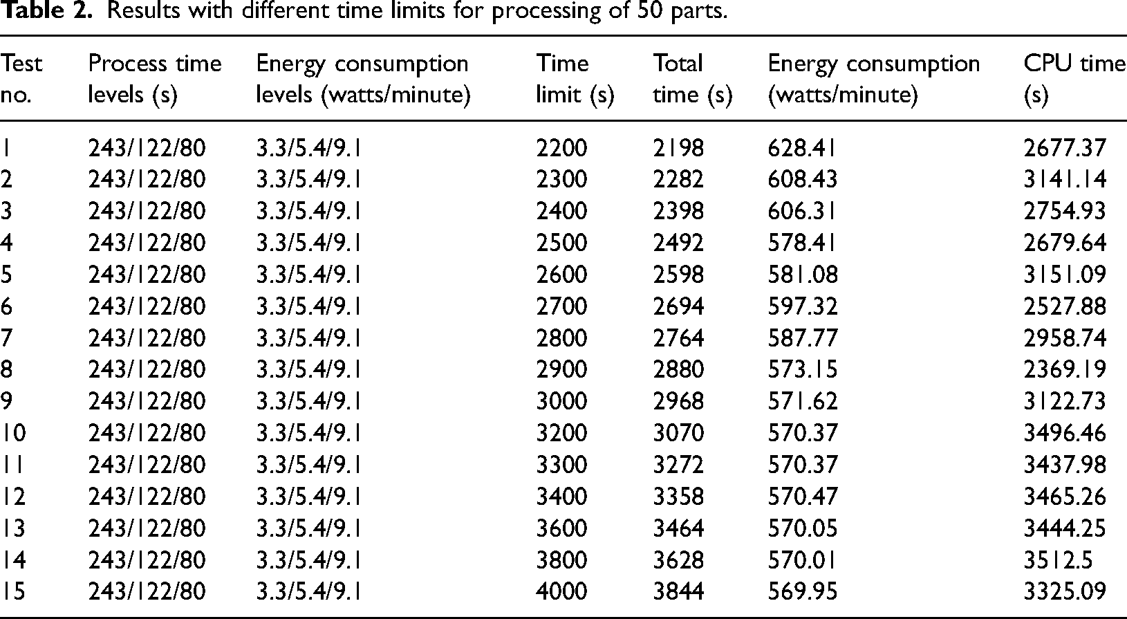
In Table 2, a time limit was considered in each step, from 2200 up to 4000 s. The results of total times show large fluctuations, between the time limit and the total time. For instance, this value for the time limit of 2200 is only 2 s (2200–2198 = 2), whereas this value for the time limit of 3800 is 172 s (3800–3628 = 172). As a general trend, it can be mentioned that with increasing the time limit, its difference with the total time is generally, not necessarily, increased. In the opposite manner, energy consumption is generally decreased by increasing the time limit of the production, which is because of utilizing a lower speed level for producing the products, in comparison with using the highest production speed level. The CPU time for solving the problems highly fluctuated at the beginning, by increasing the time limit from 2200 to 2900, but after that it increased meaningfully from 3000 up to 3800, followed by decreasing value for 3900 and 4000.

Figure 5 illustrates the trend of total times and the time limits for the 15 numbered test problems given in Table 2. As mentioned before, the time limits are growing from 2200 up to 4000 s. However, the trend of increasing the total time is not uniform. The trend of both parameters and the differences among them illustrate that with increasing the time limit, the total time is increasing.

Figure 5.

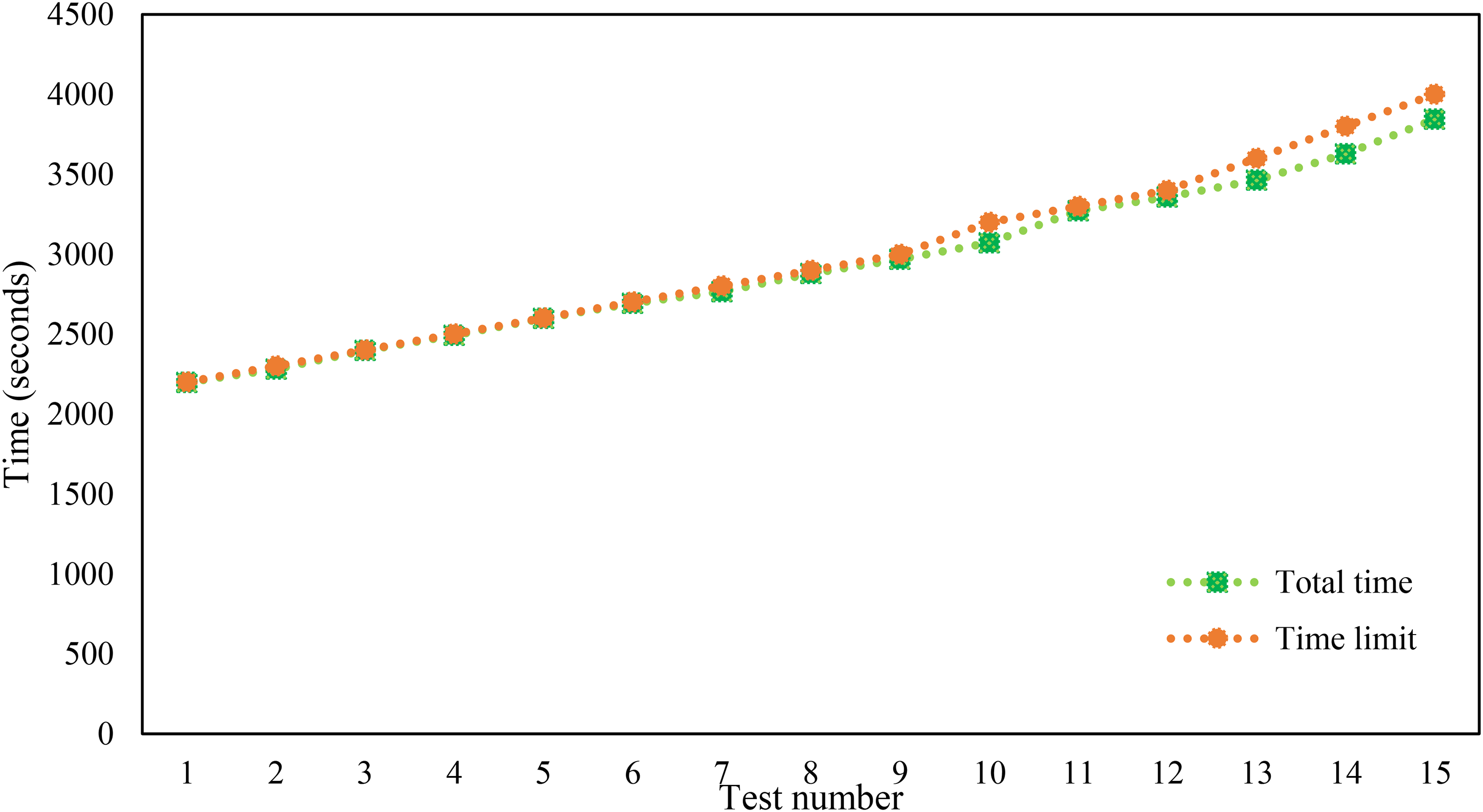
Trend of total time based on the time limit.

Figure 6 illustrates the trend of energy consumption based on the time limitation. In Figure 6, it is seen that with increasing the time limit, the energy consumption decreases, generally. However, in the beginning, with increasing the time limit from 2200 to 2900, the energy consumption decreased rapidly, with fluctuations, but for time limits above 3000, the energy consumption has a very decrement with small fluctuations from 573.15 to 569.81.

Figure 6.

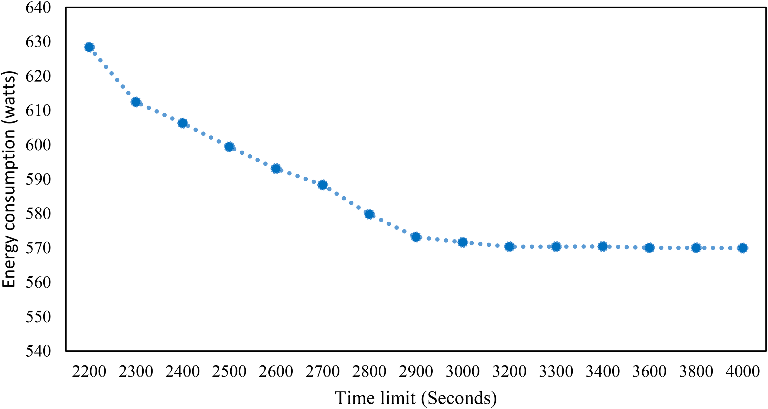
Trend of energy consumption based on the time limitation.

Figure 7 depicts the trend of CPU time based on the time limits. The figure shows high fluctuations in the CPU time in the first half of the diagram, from 2200 up to 3200 s of time limits, but thereafter, the CPU time converges to 3400 s. In the last level of the time limit, a time limit of 4000 s, the CPU time is dropped.

Figure 7.

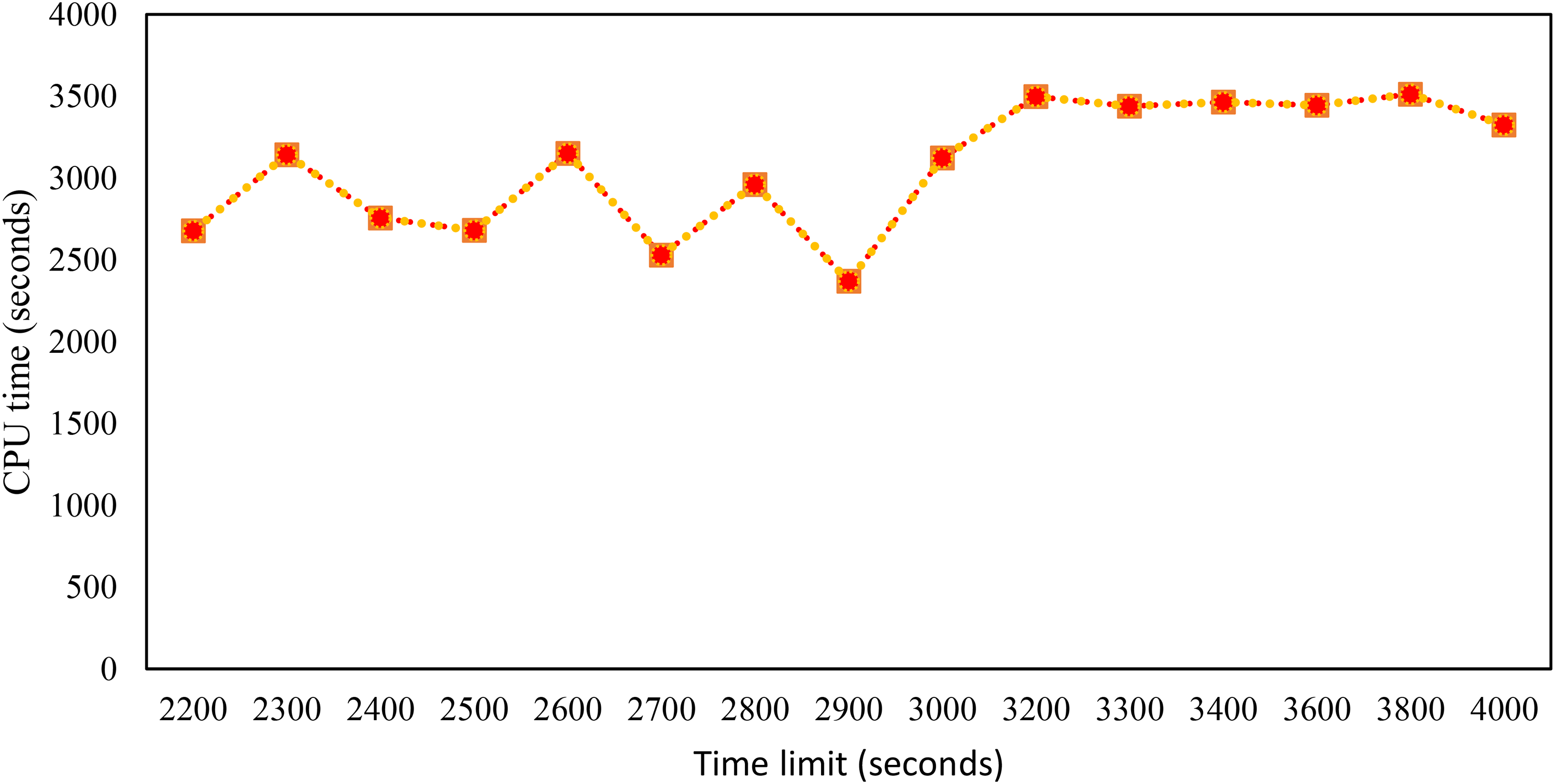
Trend of CPU time based on the time limitation.

Considering the results shown in Figures 5 to 7 in a frame gives a deeper understanding of the effect of using a time limit on the obtained results. In the first view, it is seen that by increasing the time limit, the shape of the graphs and the trend of the results change from 2900 time units. In Figure 5, up to 2900 time units, both curves are fitted to each other, and thereafter the differences will appear. In Figure 6, the graph reached a steady state after a sharp decline, and in Figure 7, it reached a steady state after some random fluctuation.

To compare the presented study with some of the most recent-related studies in a similar field, the studies performed by Wang et al.,¹⁷ Nejad et al.,⁴³ and Rubio et al.⁵¹ have been considered. The similarities and differences between the systems with what has been considered in this study are mentioned in Table 3.

Table 3.

Comparing the considered FRC with a novel system from the literature.

Specification	Presented study	Wang et al.¹⁷	Nejad et al.⁴³	Rubio et al.⁵¹
Production system	Parallel machines	Single machine	Parallel machines	Assembly line
Objectives	Energy consumption minimization	Traveling path minimization	Cycle time minimization	Cost minimization and energy efficiency maximization
Material handling system	Grounded mobile robots	Robot Manipulator	Grounded mobile robots	Automated guided vehicles
Complexity	Production time limits, speed level selection, scheduling of the robot activities sequences	Multimanipulator, maximizing operating space, multiple traveling salesman problem	Production time limits, scheduling of the robot activities considering in/out buffers of machines	Trade-off between profits and product manufacturing times
Applicability	Real-case workshops logistics	Real-case workshops and large objects	Real-case workshops logistics	Real-case factory logistics

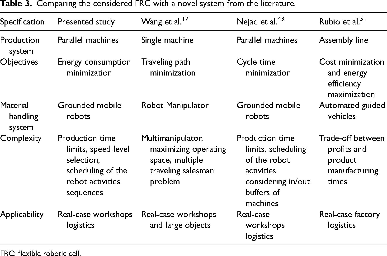
FRC: flexible robotic cell.

Conclusion

In this work, an FRC was used for the processing of a specified demand for a certain part. The machines were arranged in a line and were able to process components at different speed levels of 1, 2, and 3. Consequently, adjusting the speed of the machines results in varying energy usage during the process. As each demand typically has a deadline for fulfillment, a time constraint was addressed, with the goal of minimizing energy use for processing the entire demand. Given that this problem falls within the category of NP-hard problems, a GA was created to tackle it. A case example involving the demand for 50 products was considered to be solved, under various time limitations. The data indicate that reducing the time limit increases total energy consumption, in general, while it has been proved that the total energy consumption can be decreased by up to 15.69%, using the proposed method. Thus, this study not only aids manufacturers in meeting their customers’ requests at the lowest possible cost and energy consumption, but it also serves as a tool for improving the sustainability and reduction of GHG emissions. The case study demonstrates how optimum process scheduling can result in a reduction in total energy costs. Such savings are essential because according to Econometrics et al.⁵² in many countries the price index has increased in real terms by more than 60% over the period in such industries. The proposed approach is immediately applicable to other energy-intensive manufacturing processes. Additionally, the optimization technique can be used in any continuous process industry with adjustable loads. If process industries reschedule their operations in accordance with changing the specified optimal schedules, the utility can achieve significant peak demand reductions. Moreover, for further studies, researchers may consider different solution algorithms such as other well-known metaheuristic algorithms, to solve the problem. Considering any other types of production systems and assembly lines can be a topic for future studies.

Footnotes

Declaration of conflicting interests

The authors declared no potential conflicts of interest with respect to the research, authorship, and/or publication of this article.

Funding

The authors received no financial support for the research, authorship, and/or publication of this article.

ORCID iD

Reza Vatankhah Barenji

Mazyar Ghadiri Nejad is an Assoc. Prof. in Productions & Operations Management at Cyprus International University, Turkey. He worked as a faculty member at Girne American University, from 2018-2023. He finished his sabbatical in the Production Department at the University of Vassa. He received his PhD in Industrial Engineering from Eastern Mediterranean University. Mazyar researches Operations Research, Production Systems, Supply Chain Management, Data Analysis, and Meta-heuristic Algorithms.

Reza Vatankhah Barenji is a Senior Lecturer with over 15 years of experience in digitalization and optimization. He holds a PhD in Mechanical Engineering and has since worked with numerous organizations across various industries to help them improve their business processes through the use of digital technology. Throughout his career, he has been passionate about leveraging technology to improve the efficiency and effectiveness of business operations. He has extensive experience in process optimization, data analysis, and the implementation of digital systems, and has worked with companies of all sizes, from small startups to large multinational corporations. He has also published numerous research papers and articles on the topics of digitalization and optimization, and has been a keynote speaker at several conferences. His expertise and insights are highly sought after, and he is frequently consulted by organizations looking to improve their operations through digital transformation. As a Senior Lecturer, he brings his wealth of experience and knowledge to the classroom, helping to prepare the next generation of professionals to tackle the challenges of the digital age. He is passionate about teaching and mentoring students, and is dedicated to helping them develop the skills they need to succeed in their careers.

Güldal Güleryüz is an accomplished Assistant Professor at Hacettepe University, specializing in Industrial Engineering with a profound expertise in production scheduling. With a strong academic background and practical experience, she brings a unique perspective to the challenges of optimizing manufacturing processes. Their research focuses on developing innovative scheduling techniques that enhance production efficiency and resource allocation. Through a combination of theoretical insights and real-world applications, she continues to contribute significantly to the advancement of production scheduling methods, preparing the next generation of industrial engineers for a dynamic and competitive landscape.

Seyed Mahdi Shavarani received his PhD degree in Industrial Engineering from Eastern Mediterranean University in 2018 and a PhD in Multi-Objective Optimization and Multi-Criteria Decision-Making in 2023 from the University of Manchester. He is currently lecturing in Business Analytics at the University of Kent. His research interests lie in operations research, particularly optimization algorithms, logistics, production systems, and applications of machine learning in OR.

References

Arets

EJMM

Van Der Kolk

Hengeveld

, et al. Greenhouse gas reporting for the LULUCFsector in the Netherlands: methodological background, update 2020 (2352–2739). 2020.

Akbar

Irohara

. Scheduling for sustainable manufacturing: a review. J Cleaner Prod 2018; 205: 866–883.

Geng

Liu

. Bi-objective re-entrant hybrid flow shop scheduling considering energy consumption cost under time-of-use electricity tariffs. Complexity 2020; 2020: 1–17.

Coca

Castrillón

Ruiz

, et al. Sustainable evaluation of environmental and occupational risks scheduling flexible job shop manufacturing systems. J Cleaner Prod 2019; 209: 146–168.

, et al. An energy-responsive optimization method for machine tool selection and operation sequence in flexible machining job shops. J Cleaner Prod 2015; 87: 245–254.

Tan

Duan

. Economic batch sizing and scheduling on parallel machines under time-of-use electricity pricing. Oper Res 2018; 18: 105–122.

Yang

Chen

Wei

, et al. Robust optimization for integrated scrap steel charge considering uncertain metal elements concentrations and production scheduling under time-of-use electricity tariff. J Cleaner Prod 2018; 176: 800–812.

Gao

Yin

, et al. Human-robot collaborative scheduling in energy-efficient welding shop. IEEE Trans Ind Inf 2023: 1–9.

Wang

Liang

Zhou

, et al. Analysis of position, pose and force decoupling characteristics of a 4-UPS/1-RPS parallel grinding robot. Symmetry (Basel) 2022; 14: 825.

10.

Hou

Zhang

, et al. A space crawling robotic bio-paw (SCRBP) enabled by triboelectric sensors for surface identification. Nano Energy 2023; 105: 108013.

11.

Saberi-Aliabad

Reisi-Nafchi

Moslehi

. Energy-efficient scheduling in an unrelated parallel-machine environment under time-of-use electricity tariffs. J Cleaner Prod 2020; 249: 119393.

12.

Zhao

Grossmann

Tang

. Integrated scheduling of rolling sector in steel production with consideration of energy consumption under time-of-use electricity prices. Comput Chem Eng 2018; 111: 55–65.

13.

Zeng

, et al. 3D trajectory optimization for energy-efficient UAV communication: a control design perspective. IEEE Trans Wireless Commun 2021; 21: 4579–4593.

14.

Min

Pan

Dai

, et al. Trajectory optimization of an electric vehicle with minimum energy consumption using inverse dynamics model and servo constraints. Mech Mach Theory 2023; 181: 105185.

15.

Meng

Zhang

Shao

, et al. MILP models for energy-aware flexible job shop scheduling problem. J Cleaner Prod 2019; 210: 710–723.

16.

Zheng

Yin

, et al. An improved iterated greedy algorithm for the distributed hybrid flowshop scheduling problem. Eng Optim 2023: 1–19.

17.

Wang

Yang

Liang

, et al. An algorithm for painting large objects based on a nine-axis UR5 robotic manipulator. Appl Sci 2022; 12: 7219.

18.

Zhao

Bai

Shi

, et al. Optimal scheduling of a byproduct gas system in a steel plant considering time-of-use electricity pricing. Appl Energy 2017; 195: 100–113.

19.

Hasnaeen

SMN

Rahman

Uddin

. Load scheduling of a refrigerated warehouse with homogeneous compressors under dynamic pricing. In 2019 1st International Conference on Advances in Science, Engineering and Robotics Technology (ICASERT), 2019, pp. 1–6. IEEE.

20.

Liu

. Scheduling uniform machines with restricted assignment. Math Biosci Eng 2022; 19: 9697–9708.

21.

Giret

Trentesaux

Prabhu

. Sustainability in manufacturing operations scheduling: a state of the art review. J Manuf Syst 2015; 37: 126–140.

22.

Cui

Liu

, et al. Thermochromic VO2 for energy-efficient smart windows. Joule 2018; 2: 1707–1746.

23.

Garwood

Hughes

O’Connor

, et al. A framework for producing gbXML building geometry from point clouds for accurate and efficient building energy modelling. Appl Energy 2018; 224: 527–537.

24.

Narciso

Martins

. Application of machine learning tools for energy efficiency in industry: a review. Energy Rep 2020; 6: 1181–1199.

25.

Bänsch

Busse

Meisel

, et al. Energy-aware decision support models in production environments: a systematic literature review. Comput Ind Eng 2021; 159: 107456.

26.

Zhang

Wang

Chen

, et al. Training effective deep reinforcement learning agents for real-time life-cycle production optimization. J Petroleum Sci Eng 2022; 208: 109766.

27.

Mouzon

Yildirim

. A framework to minimise total energy consumption and total tardiness on a single machine. Int J Sustain Eng 2008; 1: 105–116.

28.

Wang

Yang

Zhang

, et al. Infinitely repeated game-based real-time scheduling for low-carbon flexible job shop considering multi-time periods. J Cleaner Prod 2020; 247: 119093.

29.

Wang

Shen

, et al. An adaptive sliding mode fault-tolerant control of a quadrotor unmanned aerial vehicle with actuator faults and model uncertainties. Int J Robust Nonlinear Control 2023: 1–17.

30.

Wang

Zhu

Han

, et al. Adaptive fault-tolerant control of a hybrid canard rotor/wing UAV under transition flight subject to actuator faults and model uncertainties. IEEE Trans Aerosp Electron Syst 2023: 4559–4574.

31.

Fang

Uhan

Zhao

, et al. Scheduling on a single machine under time-of-use electricity tariffs. Ann Oper Res 2016; 238: 199–227.

32.

Cheng

Chu

Liu

, et al. Bi-criteria single-machine batch scheduling with machine on/off switching under time-of-use tariffs. Comput Ind Eng 2017; 112: 721–734.

33.

Tan

Yang

H-l

Duan

, et al. Optimizing production scheduling of steel plate hot rolling for economic load dispatch under time-of-use electricity pricing. Math Probl Eng 2017; 2017: 1–14.

34.

Song

, et al. Model and algorithm for planning hot-rolled batch processing under time-of-use electricity pricing. Processes 2020; 8: 42.

35.

Wang

Zhu

Fang

, et al. Scheduling on a two-machine permutation flow shop under time-of-use electricity tariffs. Int J Prod Res 2018; 56: 3173–3187.

36.

Hnaien

Dugardin

. Electricity cost minimisation for optimal makespan solution in flow shop scheduling under time-of-use tariffs. Int J Prod Res 2020: 1–27.

37.

Ding

J-Y

Song

Zhang

, et al. Parallel machine scheduling under time-of-use electricity prices: new models and optimization approaches. IEEE Trans Autom Sci Eng 2015; 13: 1138–1154.

38.

Cheng

Chu

Zhou

. An improved model for parallel machine scheduling under time-of-use electricity price. IEEE Trans Autom Sci Eng 2017; 15: 896–899.

39.

Zhang

Pan

, et al. Two-stage parallel speed-scaling machine scheduling under time-of-use tariffs. J Intell Manuf 2020: 1–22.

40.

Nejad

Güden

Vizvári

. Time minimization in flexible robotic cells considering intermediate input buffers: a comparative study of three well-known problems. Int J Computer Integr Manuf 2019; 32: 809–819.

41.

Nejad

Kovács

Vizvári

, et al. An optimization model for cyclic scheduling problem in flexible robotic cells. Int J Adv Manuf Technol 2018; 95: 3863–3873.

42.

Ghadiri Nejad

Güden

Vizvári

, et al. A mathematical model and simulated annealing algorithm for solving the cyclic scheduling problem of a flexible robotic cell. Adv Mech Eng 2018; 10: 1687814017753912.

43.

Nejad

Shavarani

Güden

, et al. Process sequencing for a pick-and-place robot in a real-life flexible robotic cell. Int J Adv Manuf Technol 2019; 103: 3613–3627.

44.

Nejad

Shavarani

Vizvári

, et al. Trade-off between process scheduling and production cost in cyclic flexible robotic cells. Int J Adv Manuf Technol 2018; 96: 1081–1091.

45.

Babu

Ashok

. Peak load management in electrolytic process industries. IEEE Trans Power Syst 2008; 23: 399–405.

46.

Uğur

Aydin

. An interactive simulation and analysis software for solving TSP using Ant Colony Optimization algorithms. Adv Eng Softw 2009; 40: 341–349.

47.

Vatankhah Barenji

Ghadiri Nejad

Asghari

. Optimally sized design of a wind/photovoltaic/fuel cell off-grid hybrid energy system by modified-gray wolf optimization algorithm. Energy Environ 2018; 29: 1053–1070.

48.

Nejad

Kashan

. An effective grouping evolution strategy algorithm enhanced with heuristic methods for assembly line balancing problem. J Adv Manuf Syst 2019; 18: 487–509.

49.

Bahlouli

Lotfi

Ghadiri Nejad

. A new multi-heuristic method to optimize the ammonia–water power/cooling cycle combined with an HCCI engine. Sustainability 2023; 15: 6545.

50.

Liu

Guo

Wang

. Integrated green scheduling optimization of flexible job shop and crane transportation considering comprehensive energy consumption. J Cleaner Prod 2019; 211: 765–786.

51.

Rubio

Llopis-Albert

Valero

. Multi-objective optimization of costs and energy efficiency associated with autonomous industrial processes for sustainable growth. Technol Forecast Soc Change 2021; 173: 121115.

52.

Econometrics

SystemTechnik

Trinomics

. Study on energy prices, costs and subsidies and their impact on industry and households. 2019.

Energy consumption optimization for sustainable flexible robotic cells: Proposing exact and metaheuristic methods

Abstract

Keywords

Introduction

Literature review

Problem definition and formulation

The developed GA

Encoding

Initial solution

Evolution

Completion time and energy consumption calculations for a given solution

Results and discussions

Conclusion

Footnotes

Declaration of conflicting interests

Funding

ORCID iD

References