Sage Journals: Discover world-class research

Abstract

The carbon emission trading scheme (ETS) and tradable green certificate (TGC) system have been widely used to encourage renewable technology and mitigate greenhouse gas emissions. Previous studies have discussed the interaction between these market-based instruments and the electricity market from a theoretical perspective. This research contributes to the literature by empirically examining the interplay of carbon market, the TGC market, and electricity market using a vector autoregressive (VAR) model to investigate the price transmission between different markets. A VAR-BEKK-GARCH model, based on discrete wavelet decomposition, was used to reveal the spillover effect between the three markets over multiple time scales. Based on evidence from the partially deregulated electricity market in South Korea, we do not find a significant short-term interaction between carbon market and the TGC market through the price transmission. However, the analysis over multiple time scales demonstrates that the return spillover between the carbon market and the TGC market is positive and bidirectional in the medium-term and long-term. In addition, the policy integration may create higher price risks to the carbon market and the TGC market, resulting from long-term risk spillovers. We explain these contrasting findings and discuss implications for the future deployment of these policies.

Keywords

Carbon trading green certificates electricity dynamic transmission spillover effects

Introduction

Market-based instruments, such as the carbon emission trading scheme (ETS) and tradable green certificate (TGC) system, have dominated the diversity in content of legitimate climate policy options since 1990’s.¹ The ETS has been associated with the TGC, which facilitates the generation of electricity from renewable energy sources (RES-E) within a broader set of policy solutions.² To meet policy objectives, the newly created carbon market and TGC market need to provide the correct price signals to market participants.³ The emergence of many market-based tools has sparked intense debate about whether they may serve cross-purposes.⁴ Skeptics and critics have concluded that the interaction between ETS and TGC may generate substantial excess costs and benefit the most emission-intensive producers.⁵

Market-based instruments are rules that rely on market signals to promote behaviours that achieve pollution control.⁶ However, the interplay of carbon reduction and renewable energy promotion policies has a significant impact, sometimes creating counter-intuitive results.² Tinbergen⁷ proposed the phenomenon of overlapping regulations. That study concluded that if the objective of a single policy was to correct a single specific market failure, introducing two or more independent policy instruments may either be redundant or unnecessarily increase policy costs. Amundsen and Mortensen⁸ found that a rise in carbon price has not had the intuitively expected beneficial influence on RES-E production, either in the short-term or long-term when ETS and TGC system are both implemented. When carbon prices increased, the RES-E was substituted for electricity generated from fossil fuel sources (FFE-E); however, greater RES-E production would result in more TGC being produced.^9,10 This may lead to a decrease in the TGC price, possibly limiting the RES-E investment in the long-term. As the expression in Schusser and Jaraitė,³ in order to reduce greenhouse gas emissions, both the EU ETS and the Swedish-Norwegian TGCs employ market-based instruments. TGC price rises as a result of rising CO₂ costs, which suggests that the aims of EU ETS do not conflict with those of the Swedish-Norwegian TGCs system in the short term. They also explained why the results do not support that there are significant overlapping regulation problems between EU ETS and Swedish-Norwegian TGC. This confirms that past studies exploring these questions have generated a controversial framework. Identifying the possible interplay between the three markets is crucial to interpreting the disparate findings. Following the relevant theoretical research, we sketch a schematic diagram of the relationship between carbon, TGC, and electricity prices in Figure 1.

Figure 1.

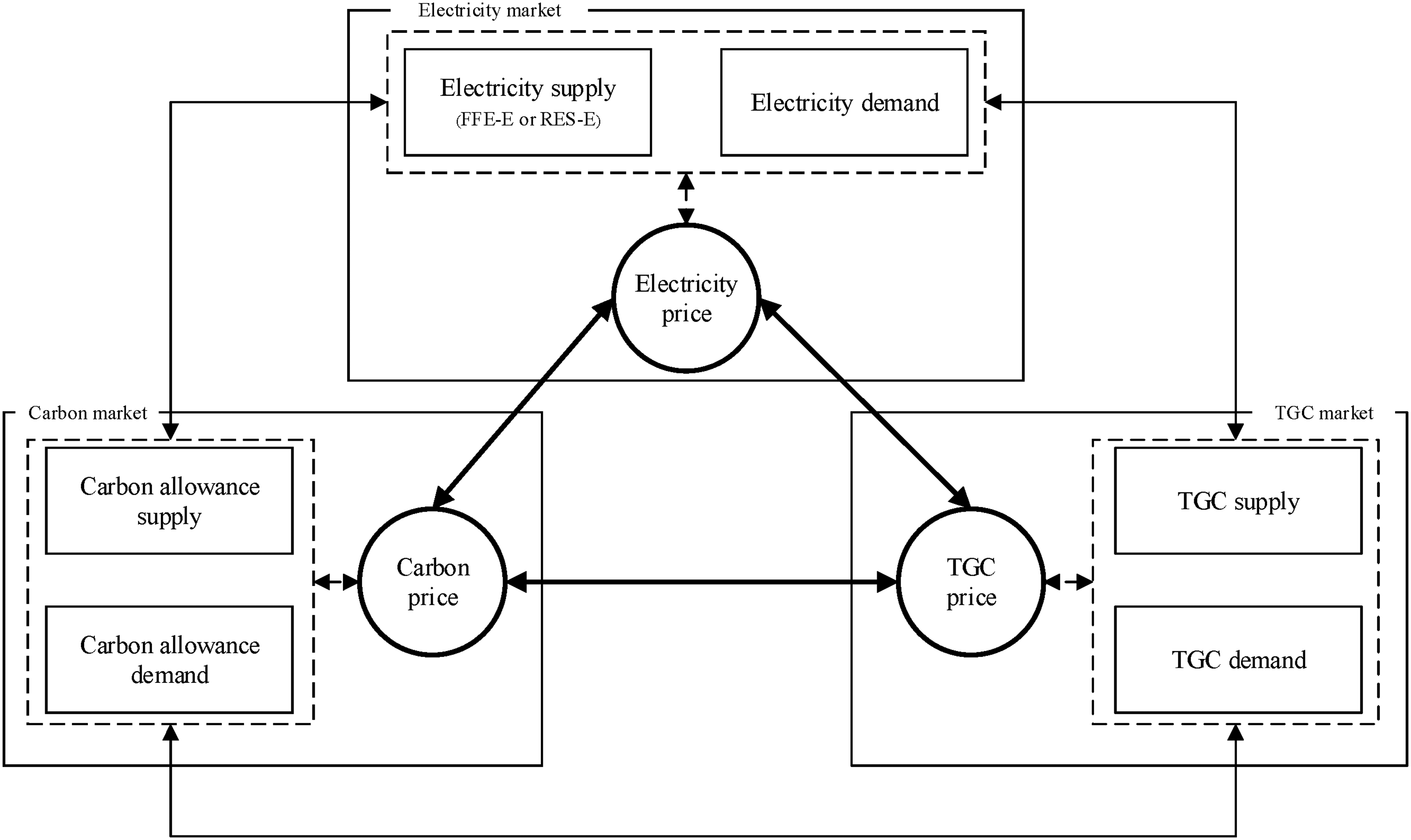
The schematic diagram of the relationship between carbon, TGC, and electricity prices.

We address the problem by exploiting the interplay of prices in a partially deregulated electricity market. The research case study is South Korea, which has introduced both carbon trading and a TGC market to achieve the decarbonization of the electricity sector. After approximately a decade of enforcement using Feed-in Tariffs, the South Korea government grew concerned about the rapid increase in the Feed-in Tariffs budget and replaced it with a Renewable Portfolio Standards (RPS) scheme in 2012. Renewable Energy Certificates (equivalent to TGC) are issued for the RES-E produced. To comply, eligible renewable units receive certificates; and electricity providers can buy the certificates or generate RES-E themselves. South Korea initiated the CO₂ emissions trading scheme in January 2015 to achieve a sustainable transition.

In addition to these actions, South Korea began transforming the operational structure of its electricity industry from a public monopoly to market competition in 1998. In April 2001, the generation sector was separated from the Korea Electric Power Corporation (KEPCO) into six generation companies. Concurrently, the Korea Power Exchange (KPX) was established to run the power industry's market pool and network infrastructure. However, following a two-thirds majority proposal from a six-member joint research panel in 2004, the Korean government postponed its reform of the electricity market.¹¹ The marketization of the electricity sector remains a controversial reform, however, ETS may lose some of its effectiveness in a partially deregulated electricity market.¹² Nevertheless, market-based instruments derived from neoclassical economic ideas play a key part in creating what Bernstein referred to as the liberal environmentalism compromise, or the adoption of liberal economic standards in international environmental policy.¹

Our paper contributes to the empirical literature by testing the potential interaction between the carbon, TGC, and a partially deregulated electricity market. Many countries and regions have partially deregulated electricity market; however, few studies have examined the interplay of prices between the market-based instruments and the electricity under such regulatory environments. We used a vector autoregressive (VAR) model to examine the interplay between the carbon market, the TGC market and the partially deregulated electricity market in South Korea. The postulated impacts of overlapping regulations have not been identified based on evidence from South Korea. However, we found the response of the electricity price to the cost of carbon is redressed, indicating excessive suppression. Furthermore, the cost created by the TGC price is not captured by the electricity price in a partially deregulated electricity market. In addition, we applied the VAR-BEKK-GARCH model based on the discrete wavelet decomposition to examine the spiller effect (return and risk spillover) between the electricity market, the carbon market, and the TGC market at multiple time scales. In practice, the policy integration may bring a higher risk of volatility, which stems from the risk spillover from the electricity market on both the long-term carbon market and the TGC market.

We present a literature review in the next section. The econometric approaches are discussed in section 3. Section 4 describes the data used in this study. The model estimation and discussion are addressed in Section 5. The final section summarizes our findings and policy implication.

Literature review

A detailed evaluation of the interaction between carbon market, the TGC market, and electricity market is an essential foundation for policy action and a criterion to adapt policy implementation. For the previous researches, dynamic price transmission and spillover effects are key concepts to consider while deconstructing this issue. As a consequence of the European Union's ETS, CO₂ emission permit payments are increasingly incorporated in sale offers and raising the cost of electricity.¹³ Rathmann¹⁴ noted that when both the policies are implemented, the wholesale price for electricity will decrease. However, the renewable support systems are usually financed through the electricity market, increasing retail electricity prices. Nevertheless, Jensen and Skytte¹⁵ found that the consumer price of electricity does not unambiguously decrease or increase by introducing TGCs. In the theoretical scope, if the introduction of TGC on the basis of ETC results in a decrease in the shadow cost of carbon emission constraints, the increased profitability of renewable energy technologies makes carbon emission caps more achievable.¹⁰ To the contrary, Schusser and Jaraitė³ found that the price of TGCs rises as the carbon price increases based on a VAR model.

On the other hand, following the contribution of Engle et al.¹⁶ and Lin et al.¹⁷ to the measurement of spillover effects, return spillover and risk spillover have been frequently employed in multi-market correlation research. In general, return spillover refers to the effect of price or return changes of one market on other markets.¹⁸ Risk spillover is to describe the impact of volatility shifting, which is often quantified as the variation of price in one market on the other.¹⁹ The carbon market may serve as a receiver in a return spillover and as a transmitter in a volatility spillover.²⁰ Despite minor changes in the underlying supply and demand factors, both the TGC market and carbon market are fundamentally vulnerable to unstable pricing.²¹ This can lead to rapid swings, from near zero values to the penalty threshold. A critical problem is created by volatility spillover between market-based instrument prices and the electricity price. To explore risk transmission, Han, Kordzakhia²² linked dynamic spillover patterns to specific short-term market events, as well as to long-term changes in the proportion of renewable energy and the installation of a carbon pricing mechanism. Gong, Shi²³ discovered significant spillover effects between the carbon and fossil energy markets, with asymmetrical intensity and direction that varied over time. Ciarreta, Pizarro-Irizar²⁴ concluded that regulatory uncertainty is linked to the time of greatest electricity price volatility. A stable regulatory policy minimizes electricity price volatility, even when renewables account for a significant part of the power market. These different studies highlight the need to further explore outstanding controversies and the interaction between the electricity market, carbon market, and green certificate markets at multiple time scales.

Furthermore, due to the financial characteristics, markets are made up of many investors, whose activities span a variety of time scales, including speculative behaviours over a few minutes and investing behaviours over several years.²⁵ There are continued debates about the different types of interplay between carbon and energy markets at different time scales. The VAR-BEKK-GARCH model is used to determine the direction of volatility spillovers between multiple markets. Wavelets are a class of mathematical functions used to decompose a signal into specific frequency components. The combination of wavelet analysis and the econometric method has been applied to examine the interaction between multiple markets.²⁶

Although past studies have made significant progress, the results are of little practical importance when assessing markets with imperfect competition. In fact, the regulatory framework may counteract the stabilizing effect expected from the competition created by the market.²⁷ A tight regulatory environment may significantly impact the price transmission of carbon, TGC, and electricity. Despite the many studies that discuss the theoretical relationship between electricity price, carbon price, and TGC price, few studies have empirically tested the relationship between the three, particularly in a partially deregulated electricity market. This type of research is needed, given the only partially deregulated status of the electricity sector in many countries. Understanding risk transmission between these markets is important for both policy makers and market investors; however, few studies have considered the possible return and risk spillover effects between carbon, TGC and electricity markets at different time scales. Therefore, we evaluated the dynamic transmission and spillover effects of carbon market, TGC market, and the partially deregulated electricity market in South Korea for the reference in policy development.

Methodology

VAR model construction

Previous studies inform the hypothesis that electricity, carbon, and green certificate prices are closely related to and influence each other in a circular way.^5,8,10 Without losing generality, we construct a standard VAR model that considers the interrelationships between the selected variables by treating them symmetrically. The basic regression model is shown in Eq. (1). A similar design is described in Schusser and Jaraitė.³

y_{t} = C + \sum_{i = 1}^{n} A_{i} y_{t - i} + μ_{t}

(1)

where

y_{t}

is the (3 × 1) vector of endogenous variables (TGC price, electricity price, and carbon price);

A_{i}

are (3 × 3) coefficient matrices for lag

i = 1, \dots, N

;

μ_{t}

is the error term with zero mean and time invariant covariance; and C is the (3 × 1) vector of constants.

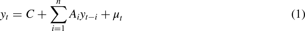
In this paper, the VAR model was used to explore the interaction among the three prices. Based on the regression, an impulse response analysis was adopted to discuss the intensity, direction, and timing of the appearance of the response to the specific price, if there were unexpected positive impacts on the other two market prices.

Multilevel time scales decomposition by discrete wavelet transform

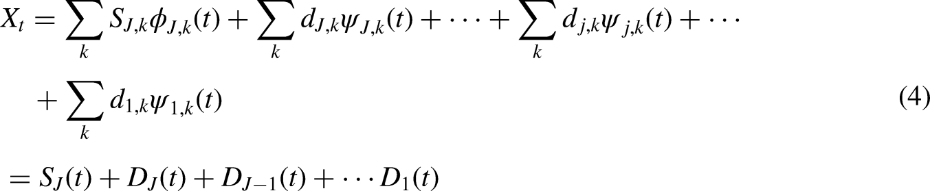
The wavelet transform provides a solution to time-related information, which is lost after decomposition (for example, an abrupt change could not be captured by the Fourier Transform). Using the definition of Ramsey and Econometrics,²⁸ the father wavelets integrate to one, and are used to represent the very long scale smooth component of the signal (generating the scaling coefficients); mother wavelets integrate to zero, and represent the deviations from the smooth components (generating the differencing coefficients).

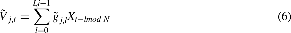
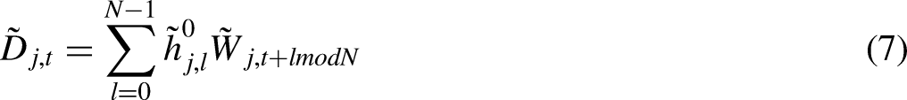
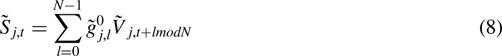
The father wavelets are shown in Eq. (2).

ϕ_{j, k} = 2^{- \frac{j}{2}} ϕ (\frac{t - 2^{j} k}{2^{j}}), \int_{- \infty}^{+ \infty} ϕ (t) d t = 1

(2)

The mother wavelets are shown in Eq. (3).

ψ_{j, k} = 2^{- \frac{j}{2}} ψ (\frac{t - 2^{j} k}{2^{j}}), j = 1, \dots, J, \int_{- \infty}^{+ \infty} ψ (t) d t = 0

(3)

Then, the original time series

X_{t}

is decomposed into:

\begin{aligned} X_{t} = \sum_{k} S_{J, k} ϕ_{J, k} (t) + \sum_{k} d_{J, k} ψ_{J, k} (t) + \dots + \sum_{k} d_{j, k} ψ_{j, k} (t) + \dots \\ + \sum_{k} d_{1, k} ψ_{1, k} (t) \\ = S_{J} (t) + D_{J} (t) + D_{J - 1} (t) + \dots D_{1} (t) \end{aligned}

(4)

Where,

D_{j} = \sum_{k} d_{j, k} ψ_{j, k} (t), j = 1, \dots J

S_{J} (t) = \sum_{k} S_{J, k} ϕ_{J, k} (t)

. The variable

D_{j}

is the detail coefficients and shows the

j^{t h}

level wavelet details associated with the variations of

X_{t}

at scale

λ_{j} = 2^{j}

. The variable

S_{J} (t)

is the smooth coefficient and presents the smoothed variations of

X_{t}

in each scale.

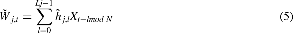
The maximal overlap discrete wavelet transform (MODWT) provides a uniform frequency band and has the property of time invariance, which is effective for working with economic data.²⁹ MODWT is used to calculate the highly redundant non-orthogonal transformation and provide the wavelet and scaling coefficients. Using Percival and Walden,³⁰ the $j^{t h}$ level MODWT wavelet and scaling coefficients can be defined as:

{\tilde{W}}_{j, t} = \sum_{l = 0}^{L j - 1} {\tilde{h}}_{j, l} X_{t - l m o d N}

(5)

{\tilde{V}}_{j, t} = \sum_{l = 0}^{L j - 1} {\tilde{g}}_{j, l} X_{t - l m o d N}

(6)

Where,

t = 0, \dots, N - 1

{{\tilde{h}}_{j, l}}

and

{{\tilde{g}}_{j, l}}

are the

j^{t h}

level MODWT wavelet and scaling filters. Then, the

j^{t h}

detail and smooth coefficients are as follows:

{\tilde{D}}_{j, t} = \sum_{l = 0}^{N - 1} {\tilde{h}}_{j, l}^{0} {\tilde{W}}_{j, t + l m o d N}

(7)

{\tilde{S}}_{j, t} = \sum_{l = 0}^{N - 1} {\tilde{g}}_{j, l}^{0} {\tilde{V}}_{j, t + l m o d N}

(8)

Where,

t = 0, \dots, N - 1

{{\tilde{h}}_{j, l}^{0}}

and

{{\tilde{g}}_{j, l}^{0}}

are the filters obtained by periodizing

{{\tilde{h}}_{j, l}}

and

{{\tilde{g}}_{j, l}}

to length N, respectively. Based on Jiang and Yoon,³¹ an asymmetric family of wavelet filters with a length L = 8 (called LA8) to was applied to conduct the wavelet decomposition. The detail coefficient

D_{j}

presents a decomposition of the original data at a time scale from

2^{j}

2^{j + 1}

. The total length of time used for this study was 202 weeks; as such, the series was decomposed into wavelet coefficients from

D_{1}

D_{5}

in our study. The

S_{6}

smooth coefficient presents a long-term trend.

VAR-BEKK-GARCH model

The VAR-BEKK-GARCH model, a multivariate GARCH model proposed by Engle and Kroner.³² It estimates the conditional mean function and the conditional volatility function of high-dimensional relationships. In this study, we used it to test the mean and volatility spillovers between electricity, carbon, and TGC market. By treating the major factors in the economic problem as endogenous variables and using the hysteresis values of all endogenous variables to create the model, the VAR model extends the univariate autoregressive to the VAR. We used the VAR(2)-BEKK-GARCH (1,1) to calculate the multiple time scale spillover effect between the electricity, carbon, and TGC markets. The VAR model was implemented to investigate the mean spillovers. The BEKK-GARCH model accounts for the volatility persistence of each market and for the own- and cross-volatility spillover effects between the markets.³³ The VAR(2)-BEKK-GARCH(1,1) model is specified as follows:

R_{t} = μ + Λ_{1} R_{t - 1} + Λ_{2} R_{t - 2} + ε_{t}

(9)

ε_{t} \sim N (0, H_{t})

(10)

H_{t} = C C^{'} + D H_{t - 1} D^{'} + B (ε_{t - 1} ε_{t - 1}^{'}) B^{'}

(11)

where,

R_{t}

is the returns matrix of the electricity, carbon, and TGC markets;

Λ_{j}

are coefficient matrices for lag

j = 1, 2

;

ε_{t}

is a 3 × 1 vector of the residual and follows a normal distribution. The variable

H_{t}

is the conditional variance-covariance matrix; C is the constant matrix and 3 × 3 lower triangular vector; and D is a (3 × 3) matrix of conditional variance, where the

d_{i j}

captures the own volatility persistence and the volatility interactions between markets i and j. The variable B is a (3 × 3) parameter matrix of residual and its element

b_{i j}

capture the ARCH effect in the residual in market i and j. We use the Wald test to test the mean and volatility spillover effect between the considered markets. To be specific, for market i and j, the Wald test hypothesize that

Λ_{j} = 0, j = 1, 2

. The rejection of the null hypothesis indicates that there is a return spillover from market i to market j. The null hypothesis of Wald test is

D (i, j) = B (i, j) = 0

. The rejection indicates that there is risk spillover from market i to market j.

Data description

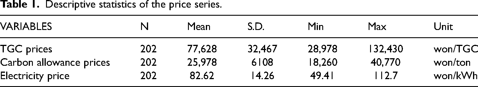
This study examined the weekly price series for TGC in the South Korea TGC system; the price of electricity in mainland Korea; and the carbon allowances in the Korean emission trading scheme. The average price of the bidding zones in Korea's major territory was used to calculate the spot price of electricity, which was determined from the Electric Power Statistics Information System. KEPCO was separated into six subsidiaries in April 2001 to achieve supply-side competition. Despite this, KEPCO purchases electricity from the pool in the retail sector as a monopolistic demand-side operator. The marginal cost of electricity generation largely determines the electricity price; however, government intervention and the monopolistic structure significant impact electricity price. The electricity market, which is monopolistic in nature and subject to government price controls, creates a significant cost-effectiveness problem for policymakers.

The weekly TGC prices in the Korean TGC system were collected from the KPX for the years 2017–2021. As noted above, concerns about the rapidly escalating expenditures for Feed-in Tariffs subsidies prompted the Korean government to introduce the RPS scheme in 2012. Under the RPS, 18 power generation companies with capacities more than 500 MW must use RES-E to generate a certain amount of their electricity. The RES-E target is expected to increase from 2% in 2012 to 10% in 2023. A power company can achieve this goal either by supplying RES-E or by acquiring TGC from the TGC market. The TGC price is vulnerable to rapid changes under RPS.³⁴ In reality, the supply and demand of TGC influence TGC pricing. TGC demand is determined by the availability of electricity, and the percentage requirement. TGC supply is determined by the number of granted TGCs. The production of RES-E is favourably linked to the issued TGCs.

The data series capturing the carbon allowance price was retrieved from the Korea Exchange. CO₂ emissions from the power sector account for approximately 30% of total emissions in South Korea, indicating the power sector's possible significant role in ETS development.³⁵ With the exception of the electricity industry, most industrial sectors are less likely to be active traders under the ETS. Power companies are the most active traders among regulated entities, due to several unique advantages in the power sector, including daily electricity trades in the wholesale market operated by KPX, real-time monitoring of fuel inputs for generation, and subsequent calculation of CO₂ emissions.

The empirical analysis was conducted using weekly data from the last week in March of 2017 to the last week in February of 2021. The data were not seasonally adjusted, as seasonal patterns were not significant in any of the data series. No further data transformations were performed. Table 1 presents the basic descriptive statistics of the data used in this paper.

Table 1.

Descriptive statistics of the price series.

VARIABLES	N	Mean	S.D.	Min	Max	Unit
TGC prices	202	77,628	32,467	28,978	132,430	won/TGC
Carbon allowance prices	202	25,978	6108	18,260	40,770	won/ton
Electricity price	202	82.62	14.26	49.41	112.7	won/kWh

Model estimation and discussion

VAR model estimation and impulse response analysis

VAR model specification and diagnostics

In this study, we used Augmented Dickey Fuller (ADF) and Phillips Perron (PP) unit root tests to assess the integration order of each variable. The results are shown in Table 2. The results are presented for a lag length of four, but are robust to changes in the lag length. The statistics associated with both the ADF and PP unit root tests indicate that all price series are integrated in an order of one, whereas the first differences reflect a stationary process.

Table 2.

Unit root tests.

	Level			First difference
	ADF^a	PP		ADF	PP
	ADF^a	Z( $ρ$ )^b	Z(t)^c	ADF	Z( $ρ$ )^b	Z(t)^c
Electricity price	−1.765	−6.268	−1.782	−5.659	−190.933	−14.408
TGC price	−0.774	−1.081	−0.714	−7.334	−104.579	−9.580
Carbon price	−1.239	−4.558	−1.444	−6.338	−141.786	−11.857

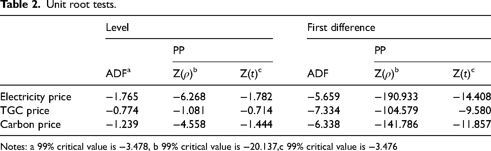
Notes: a 99% critical value is −3.478, b 99% critical value is −20.137,c 99% critical value is −3.476

Table 3 shows the lag length test results. With the exception of the Schwarz’s Bayesian information criterion (SBIC), the Final prediction error (FPE) shows that the Akaike’s information criterion (AIC) and Hannan and Quinn information criterion indicate that two lags should be used to estimate the VAR model. Therefore, this paper estimates the model with two order lags.

Table 3.

VAR lag order selection criteria.

lag	LL	LR	df	p	FPE	AIC	HQIC	SBIC
0	978.729				1.0e–08	−9.906	−9.886	−9.856*
1	997.057	36.656	9	0.000	9.1e–09	−10.001	−9.920	−9.801
2	1023	51.883*	9	0.000	7.7e–09*	−10.1726*	−10.0309*	−9.823
3	1026.320	6.636	9	0.675	8.1e–09	−10.115	−9.912	−9.615
4	1031.830	11.026	9	0.274	8.4e–09	−10.079	−9.816	−9.430

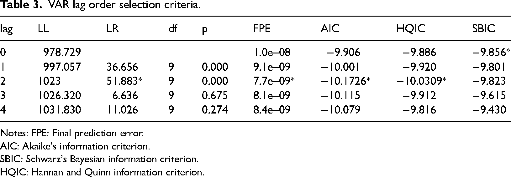
Notes: FPE: Final prediction error.

AIC: Akaike's information criterion.

SBIC: Schwarz's Bayesian information criterion.

HQIC: Hannan and Quinn information criterion.

We conducted a co-integration test based on the VAR model. The results in Table 4 show that there are three cointegration relationships between the variables based on five different test type.

Table 4.

Number of cointegrating relations.

	None	None	Linear	Linear	Quadratic
Test Type	No Intercept	Intercept	Intercept	Intercept	Intercept
	No Trend	No Trend	No Trend	Trend	Trend
Trace	3	3	3	3	3
Max-Eig	3	3	3	3	3

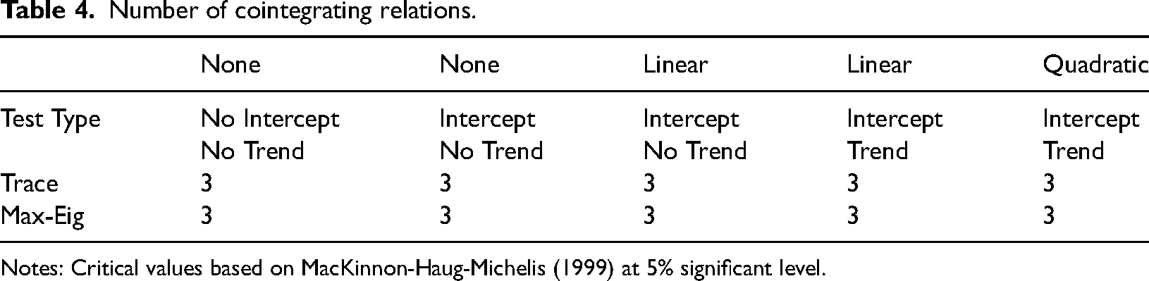
Notes: Critical values based on MacKinnon-Haug-Michelis (1999) at 5% significant level.

The roots of the characteristic polynomial were calculated to ensure the stability of the VAR model. Figure 2 shows that all the inverse roots of the AR characteristic polynomial are in the unit circle. This demonstrates that the VAR model is stable.

Figure 2.

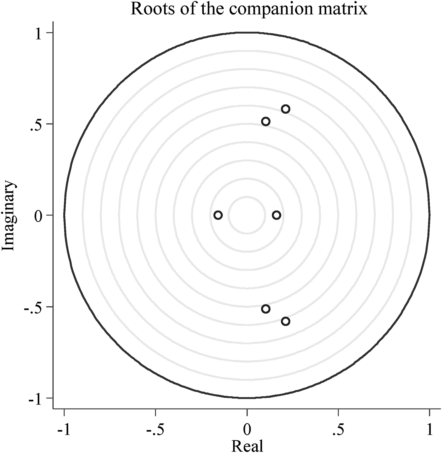
Inverse roots of AR characteristic polynomial.

Impulse response analysis

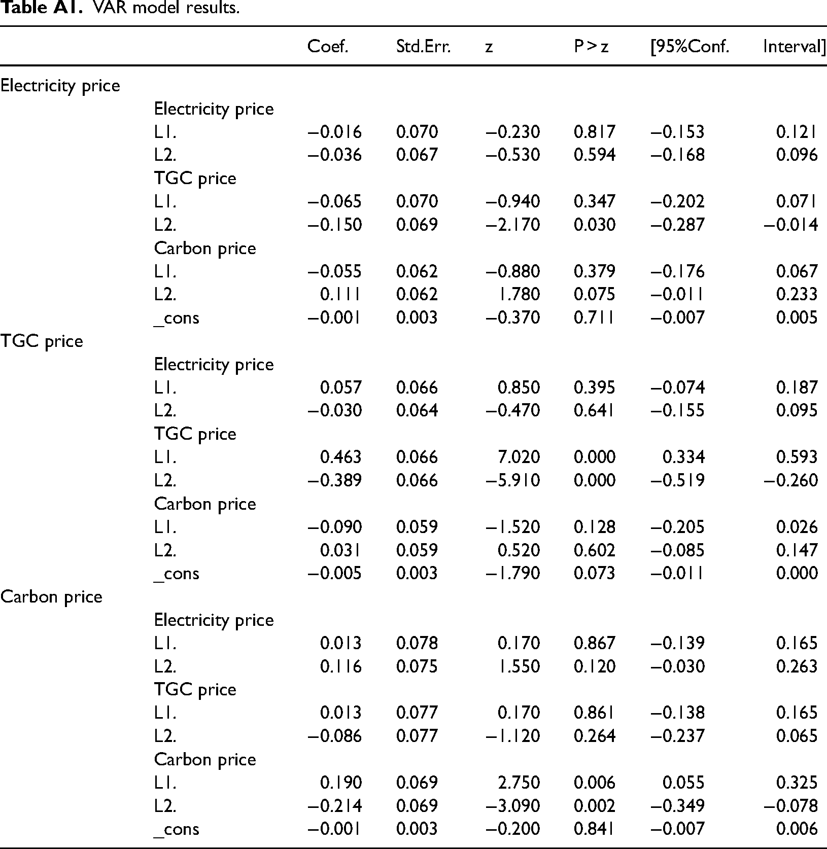
The detailed results of the estimated VAR model are presented in Appendix A. We investigated the interplay of the three prices, by estimating the impulse response functions to investigate the dynamic properties of the VAR system. The changes on the y axis indicate how individual variables respond to other endogenous shocks. The legend indicates the response variables. The pattern in the Figures 3(a)–5(b) is determined by the estimate results of VAR Models and the impulse response function choices. We collect all the impulse response results in one sheet in the Appendix B.

Figure 3.

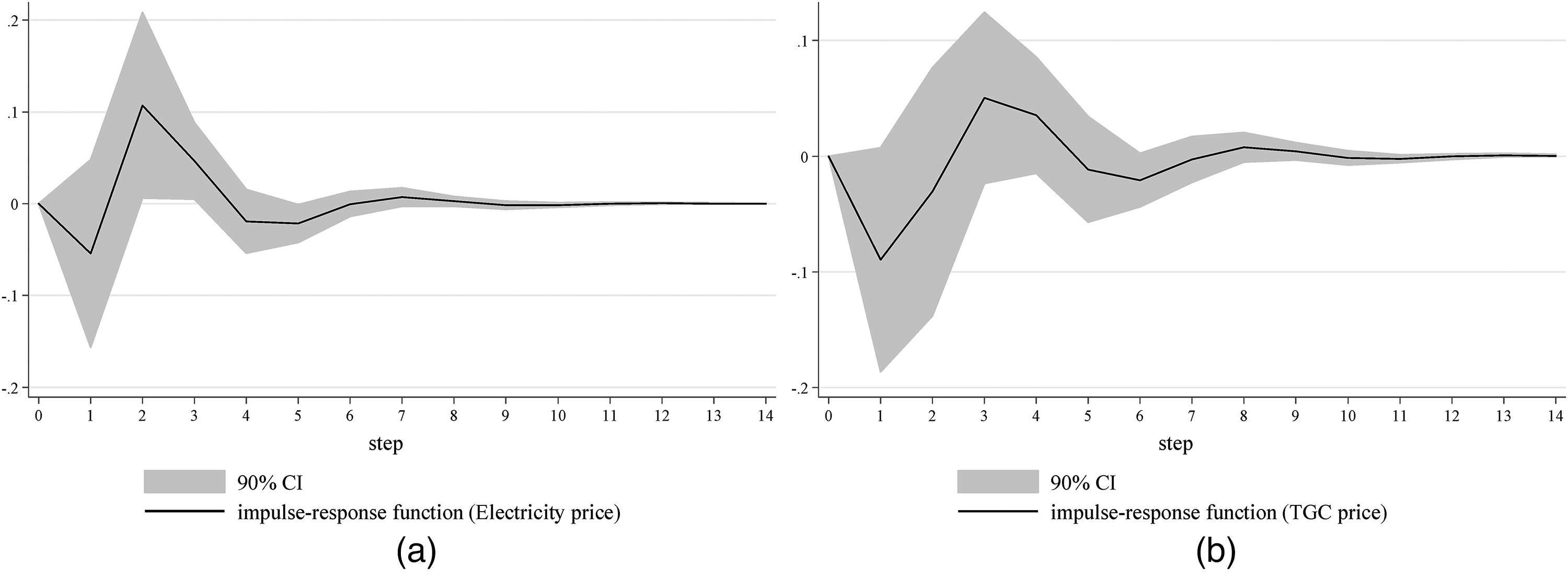
(a) Response of electricity price to a shock to carbon price. (b) Response of TGC price to a shock to carbon price.

Figure 5.

(a) Response of carbon price to a shock to electricity price. (b) Response of TGC price to a shock to electricity price.

Figure 3(a) shows the impulse responses of the electricity price from a positive one-standard deviation shock in the carbon price. This type of shock can arise from an economic expansion, which results in an increase in demand for the products from the industries regulated under ETS.³⁶ The shock may be derived from the plan that tries to reduce the total carbon allowances, which may fulfil the expectations of a shrinking supply of carbon allowance.³⁷ The expected shock in carbon price significantly positively impacts the electricity piece in the second and third week. However, the response is temporary and becomes negative in the fifth week. This may be due to the partially deregulated feature of the Korean power market. KEPCO was split into six distribution businesses to establish wholesale market competition; however, KEPCO remains the sole purchaser of electricity (electricity retail business). Therefore, competition is allowed in the supply side, but there is a monopoly on the demand side. The electricity price shows short-term fluctuation, instead of a continuous increase when the cost of generating FFE-E rises.

Figure 3(b) shows that the shock to carbon price has a negative effect on TGC price in the first two weeks, but becomes positive in the following two weeks. However, the responses are insignificant for all horizons. These results differ from previous empirical evidence and theoretical considerations. Previous studies have found that when carbon prices increase, the RES-E is substituted for FFE-E, changing the electricity supply structure and influencing the TGC price. In the context of the South Korea TGC system, the strictly regulated electricity price blocks the cost pass-through in the electricity trading market and in the carbon market.³⁵ As a result, the ETS cannot function to reduce the cost gap between producing the FFE-E and the RES-E. Likewise, the merit order effect is distorted by the price interference. Therefore, this test indicates that changes in the carbon price do not significantly influence the electricity supply structure in a strictly regulated environment.

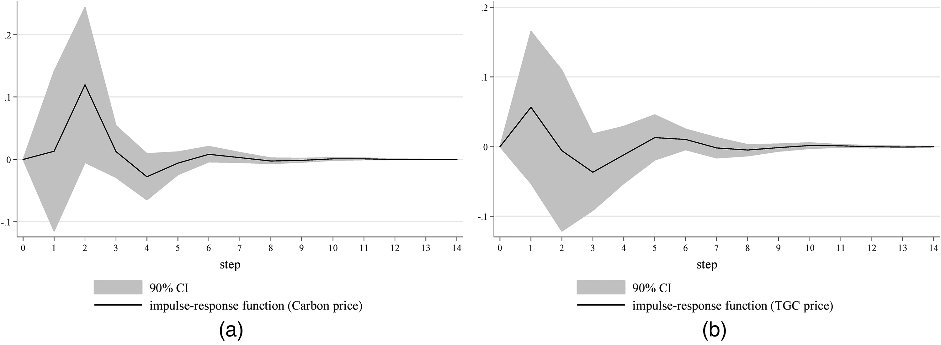
Figure 4(a) presents the impulse responses in carbon prices from a positive one-standard deviation shock in TGC price. Such a shock can arise with a higher tuning of the annual obligation requirements³⁸ or lower availability of RES-E due to weather.³⁹ Figure 4(a) shows that a shock in the TGC price has a fairly small positive effect on carbon price in the first week, but becomes negative in the following three weeks. However, these results are not significant for the entire time horizon. These results are consistent with Schusser and Jaraitė³ who hypothesized that the size of the TGC market is too small compared to the carbon market to generate a significant sustained change. Electricity companies are the most active traders among regulated entities under the ETS in South Korea³⁵; however, the TGC price also did not significantly impact carbon prices in the short-term. In addition to the differences in relative size, this phenomenon may be explained by the low contribution of the potential expansion of RES-E to carbon emission reductions in the power sector. Although the increase in the TGC price may stimulate the substitution of RES-E for the FFE-E, strong growth in electricity demand will also incentivize a potential FFE-E supply due to electricity price regulation in South Korea.

Figure 4.

(a) Response of carbon price to a shock to TGC price. (b) Response of electricity price to a shock to TGC price.

Figure 4(b) shows how the electricity price responds when the TGC price experiences a positive shock. In contrast to the findings of Schusser and Jaraitė,³ our results indicate that the electricity price shows a negative, though insignificant, response in the first week, but becomes significantly negative in the second week. This phenomenon may be due to the insufficient substitutability of the supply of RES-E on the electricity supply from fossil fuel. Kim and Chang⁴⁰ stressed that renewable technologies show an overstated learning capacity, which is partially inconsistent with South Korea's technological setting, in which nuclear energy could potentially serve as a primary substitute. In addition, the larger electricity suppliers with an RPS obligation have generally fulfilled their requirements by producing more RES-E.⁴¹ After adjusting the RES-E supply due to the positive shock to TGC price, the possible increase in supply of RES-E may place downward pressure on the electricity price, if the increased renewable energy power does not substitute the FFE-E.

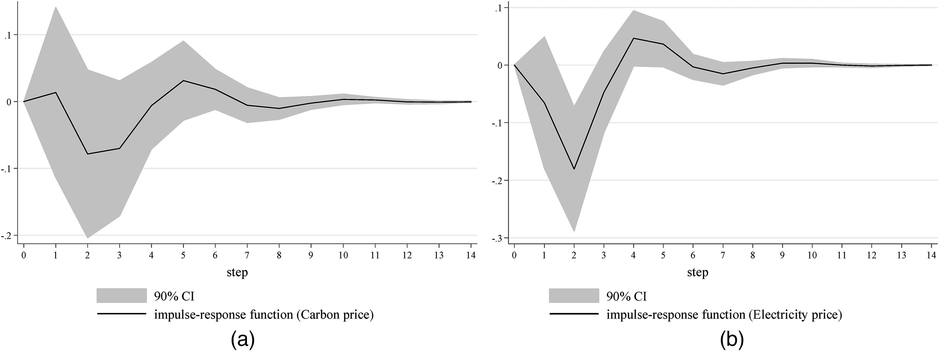
Figure 5(a) presents the impulse responses in carbon prices from a positive one-standard deviation shock in the electricity price. Electricity price shocks are often loosely motivated by shocks to electricity demand (e.g., temperature changes) or by shocks to an inelastic electricity supply (e.g., production or system breakdowns).⁴² In Figure 5(a), the carbon price shows a positive, though insignificant, response to the shock to electricity price in the first three weeks; however, the response becomes negative in the fourth week. The rise of electricity price may simultaneously stimulate the supply of RES-E and FFE-E. This may result in an insignificant increase in potential carbon demand, because the two kinds of electricity may share the potential incremental market.

Figure 5(b) presents the impulse responses in the TGC price from a positive one-standard deviation shock in the electricity price. The TGC price shows a positive response to the shock to electricity price at the first week; however, it becomes negative in the following three weeks. The value is insignificant across time horizons. Schusser and Jaraitė³ hypothesized that an increase in electricity price will reduce electricity demand, as well as the demand for green certificates, leading to a lower TGC price. In addition, as discussed above, an increase in electricity price may not significantly change the proportion of renewable electricity in the total electricity supply. The response of the TGC price to changes in the electricity price may depend on the substitutability of the RES-E to FFE-E through incremental competition.

VAR-BEKK-GARCH model estimation at multi-time scales

Mean spillover at multi-time scales

Based on the MODWT, we decomposed the original series into five detail wavelet coefficients from $D_{1}$ to $D_{5}$ and smooth coefficient $S_{6}$ . The discrete wavelet transform can be conceived of as a method for subsampling on dyadic scales. $D_{j}$ picks times from $2^{j}$ to $2^{j + 1}$ $(j = 1, \dots, 5)$ weeks scale and captures the features of specific frequency sample motions. High-frequency motions of the 2 to 4 weeks scale are represented by $D_{1}$ . A sample motion with a relatively low frequency is represented by $D_{5}$ . The similar design can be found in Jiang and Yoon.³¹ Table 5 shows the time scales (or horizon) of each $D_{j}$ used in the estimation of VAR-BEKK-GARCH model. The ADF test and ARCH test for each series can be found in Appendix C.

Table 5.

The time scales (or horizon) of the detail coefficients in wavelet decomposition.

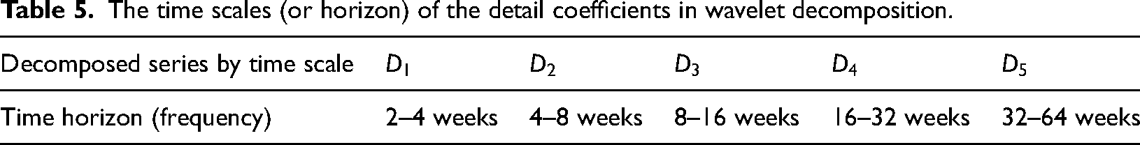
Decomposed series by time scale	$D_{1}$	$D_{2}$	$D_{3}$	$D_{4}$	$D_{5}$
Time horizon (frequency)	2–4 weeks	4–8 weeks	8–16 weeks	16–32 weeks	32–64 weeks

The detailed estimation results of the mean function to VAR-BEKK-GARCH model are presented in Appendix C. As discussed above, the Wald test was used to determine if there is return spillover from market i to market j. The results are shown in Table 6.

Table 6.

Wald test of mean spillover between the three markets at the specific multi-time scales.

	Electricity market	Carbon market	TGC market
$D_{1}$ (2–4 weeks)
Spillover from electricity market to		0.839	0.613
Spillover from carbon market to	2.576*		0.402
Spillover from TGC market to	0.065	0.952
$D_{2}$ (4–8 weeks)
Spillover from electricity market to		3.121**	12.435***
Spillover from carbon market to	3.489**		3.919**
Spillover from TGC market to	0.482	6.834***
$D_{3}$ (8–16 weeks)
Spillover from electricity market to		5.750***	9.907***
Spillover from carbon market to	2.136		8.589***
Spillover from TGC market to	25.828***	3.931**
$D_{4}$ (16–32 weeks)
Spillover from electricity market to		4.430**	6.260***
Spillover from carbon market to	20.715***		20.010***
Spillover from TGC market to	2.013	3.646**
$D_{5}$ (32–64 weeks)
Spillover from electricity market to		5588.485***	237.861***
Spillover from carbon market to	385.857***		190.944***
Spillover from TGC market to	236.669***	318.516***

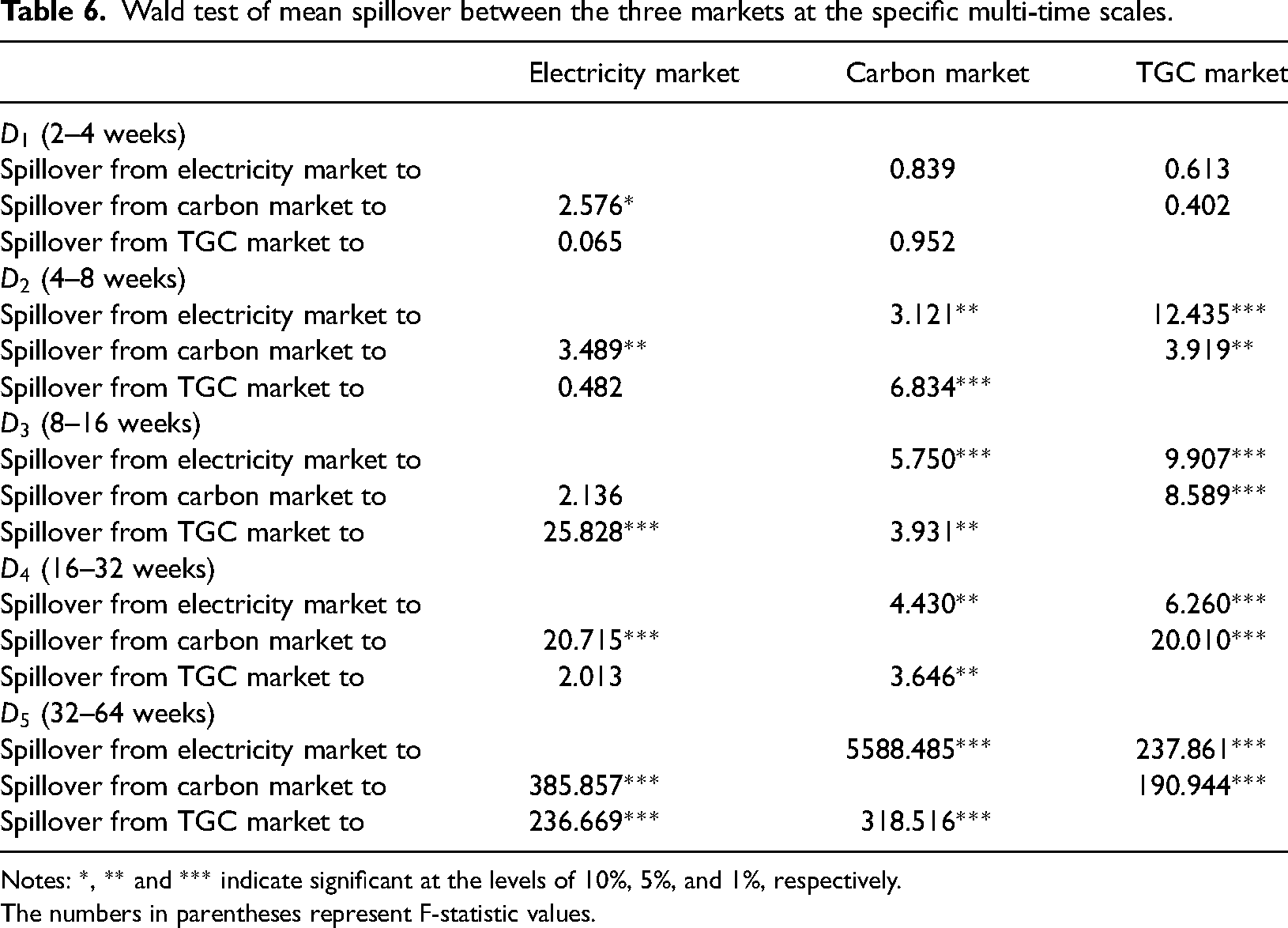
Notes: *, ** and *** indicate significant at the levels of 10%, 5%, and 1%, respectively.

The numbers in parentheses represent F-statistic values.

Our results demonstrate that in a short-term horizon (2–4 weeks), there is no significant mean spillover among different markets with one exception: a positive mean spillover from the carbon market to the electricity market, these results are similar to the findings in Section 3. This can be explained by the fact that government regulation can restrict price fluctuations. Both emission reduction investment and the growth of installed renewable energy capacity are challenging to play a part in a short period of time.^43,44 As a result, carbon price changes are unlikely to have a substantial influence on renewable energy production in a short period of time. Similarly, short-term fluctuations in the price of TGC have little discernible effect on the relatively large carbon market. However, in the medium-term and long-term horizons, there may be significant mean spillover effects among different markets. Specifically, the positive mean spillover between the carbon market and the TGC market is positive and bidirectional in the medium-term and long-term (4–64 weeks). To avoid large short-term increases in the cost of power or environmental protection, the government generally implements price-control measures. However, a cost shock may not be avoidable, even when there is a long-term price control system.⁴⁵ Therefore, our results demonstrate that the ETS and TGC policies do not produce the theoretically overlapping regulatory problems, where an increase in the carbon price would lead to a decrease in the TGC price and limit long-term RES-E investments. These findings can be explained as follows. The increase in carbon prices usually stems from a growth of carbon demand created by economic expansion. Likewise, energy resources and economic growth tend to create a positive feedback loop, locking an economy into specific consumption patterns.⁴⁶ Potential electricity price regulation restricts the demand response.⁴⁷ Therefore, due to the limited supply capacity of RES-E and the insufficient substitutability of the RES-E for FFE-E, the demand for the TGC may increase, which is accompanied by an increase in the carbon price.

In contrast, the Electricity Market Operation Council in South Korea serves as an expert group that performs this cost review role. The Council is a non-profit body that makes objective and fair judgements on topics pertaining to the Electricity Market Operation Rules. The Council holds monthly meetings with its chairman and eight members to ensure careful attention when amending or establishing processes, and relevant elements are evaluated in a fair and open manner. The current electricity market is a Cost Based Pool, which means the market price is determined by calculating costs from each generator's variable expenses. Therefore, the response of the electricity market to spillovers from the carbon market and the TGC market is volatile within specific time scales. The response of the electricity market depends on the committee's targets in a defined time scale.

Risk spillover at multi-time scales

Detailed estimation results of the conditional variance-covariance matrix and matrix of residual are presented in Appendix C. As discussed above, the Wald test was applied to determine whether there is a risk spillover from market i to market j. The results are shown in Table 7.

Table 7.

Wald test of volatility spillover between the three markets at the specific multi-time scales.

	Electricity market	Carbon market	TGC market
$D_{1}$ (2–4 weeks)
Spillover from electricity market to		2.035	14.368***
Spillover from carbon market to	1.445		5.740***
Spillover from TGC market to	0.607	2.088
$D_{2}$ (4–8 weeks)
Spillover from electricity market to		2.310*	14.690***
Spillover from carbon market to	1.037		3.572**
Spillover from TGC market to	7.946***	0.354
$D_{3}$ (8–16 weeks)
Spillover from electricity market to		0.222	4.386**
Spillover from carbon market to	1.096		4.722***
Spillover from TGC market to	0.166	1.076
$D_{4}$ (16–32 weeks)
Spillover from electricity market to		1.840	9.032***
Spillover from carbon market to	8.086***		5.706***
Spillover from TGC market to	1.662	3.859**
$D_{5}$ (32–64 weeks)
Spillover from electricity market to		67.428***	36.015***
Spillover from carbon market to	10.320***		1.127
Spillover from TGC market to	12.320***	23.529***

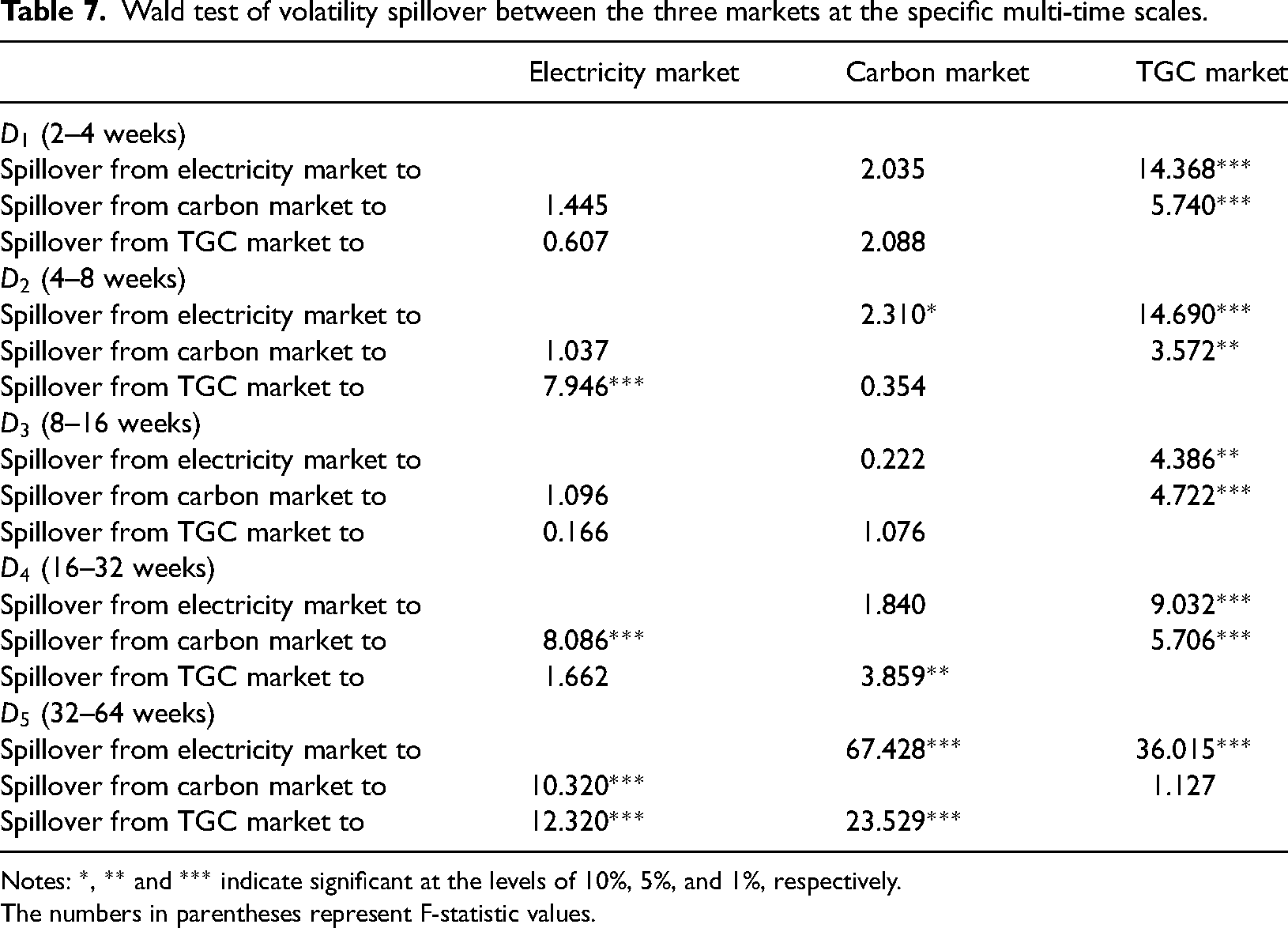
Notes: *, ** and *** indicate significant at the levels of 10%, 5%, and 1%, respectively.

The numbers in parentheses represent F-statistic values.

When considering the risk spillover at multiple time scales between the three markets, the TGC market becomes the main risk receiver. This means that the TGC market is mitigated by the risk from other markets at a time scale of less than 32 weeks. This means that risk in any market may evolve into price fluctuations in the TGC market. In other words, besides the endogenous policy uncertainty, the TGC market may experience greater market risks due to overlapping regulation. The risk spillover between the carbon market and the TGC market is unidirectional at a time scale shorter than 16 weeks. However, the spillovers between the carbon market and the TGC market are bidirectional in the time-scale of 16–32 weeks. This may be because the size of the TGC market is smaller than the size of the carbon market. The uncertainty of carbon prices may pass risks to the TGC market by adjusting the supply strategy of relevant electricity companies. However, companies in other industries may not adjust their investment of carbon allowance due to the short-term fluctuations in TGC price. In contrast to short-term investment behaviours, long-term investment behaviours are more likely to reflect the potential impact of renewable energy deployment on carbon emissions, because the electricity sector is the main source of carbon emissions.⁴⁸ Therefore, the volatility of the TGC market may spill over to the carbon market in the long-term. However, each generation of carbon allowances usually lasts one year; as such, the response of the TGC market to the risk in the carbon market becomes insignificant when the time scale is too long.

In addition, the risk spillover of the electricity market on the other two markets also differs between the different time scales. In the short-term or medium-term (2–4 weeks, 8–32 weeks), the risks in the electricity market have no spillover effects on the carbon market. This may be because participants in the carbon market do not change their investment behaviour to mitigate the potential threats caused by fluctuations in the electricity price. However, in the long-term, an increase in electricity price could lead to an increase in the number of patents associated with renewable energy technologies.⁴⁹ Lin and Chen⁴⁹ stressed that a higher electricity price could make renewable energy more competitive. Therefore, the electricity market may have a risk spillover effect on the carbon market in the long-term (32–64 weeks).

Conclusion and policy implications

There are few econometric analyses of the price interaction of carbon, TGC and electricity under partially deregulated environment, though the insufficient electricity market liberalization reform is ubiquitous across the world. We used evidence from South Korea to perform a standard VAR and MODWT-based VAR-BEKK-GARCH analysis. This case study country has a partially deregulated electricity sector, providing crucial evidence about the interaction of the three markets. Three areas need to be prioritized. The first is that the short-term interplay between the carbon and TGC markets may need to be re-examined in the future. The second is the pricing method for electricity in a partly deregulated market. The third is the control of long-term risk arising from policy tool overlap.

Our results did not find a significant interaction between the carbon price and green certificate price in the partially deregulated market environment in a short run. As such, we conclude that an increase in carbon prices does not significantly impact the electricity supply structure. This finding demonstrates that the polices of ETS and TGC have retained a high degree of independence in the short term. Therefore, we recommend gradually reducing carbon quotas and increasing the targeted share of renewable electricity, to achieve the decarbonization in the electricity sector in a short term. However, as the substitutability of renewable energy improves, the interaction between the carbon market and the TGC market may need to be re-examined.

Second, the response of the electricity price to a shock to the carbon price was not continuously positive as hypothesized, potentially generating a significant negative response. This means the demand response in the electricity sector from rising carbon prices may be limited. Furthermore, the electricity price shows a significant negative response to the shock in the TGC price, indicating that the substitutability of RES-E to FFE-E may be insufficient. An increase in RES-E can only achieve an increase in electricity supply. Therefore, any increase in the requirement to obligate a proportion of quotas to the TGC system may become a policy choice to curb the increase in the electricity price in a short run. However, in the long term, it is critical to enhance the substitution of renewable energy for fossil energy through a more flexible method for setting electricity prices in a partially deregulated electricity market.

Third, the positive mean spillover between the carbon market and the TGC market is bidirectional in the medium and long term (4–64 weeks). This means that the green quota imposed on top of the ETS would not encourage electricity production using high carbon emission technologies. However, policy integration may bring higher risks to the carbon market and TGC market, which stem from long-term risk spillovers. From a policy perspective, the simultaneous implementation of ETS and TGC in the electricity sector is still feasible in the long run. However, we recommend that the government strengthen its long-term risk management of the carbon market and TGC market. These actions are needed to control risk spillover when a risk event occurs in either the carbon market or the TGC market.

The results of this work are influenced by the characteristics of the samples utilized in the study. The three markets’ supply and demand are likely to interact in the near future, necessitating additional theoretical research and data analysis to explain the phenomenon.

Footnotes

Declaration of conflicting interests

The author(s) declared no potential conflicts of interest with respect to the research, authorship, and/or publication of this article.

Funding

The author(s) disclosed receipt of the following financial support for the research, authorship, and/or publication of this article: This work was supported by the China Scholarship Council, Postgraduate Research & Practice Innovation Program of Jiangsu Province, National Natural Science Foundation of China, Fundamental Research Funds for the Central Universities, (grant numbers 202006830108, KYCX20_0232, 71834003, 72074111, NE2018105).

ORCID iD

Changsong Wu

Changsong Wu is a PhD student in the College of Economics and Management at Nanjing University of Aeronautics and Astronautics, Nanjing, Jiangsu, China. He is also a research associate at Seoul National University's Institute for Sustainable Development. His core research area is energy economics.

Dequn Zhou is professor in the College of Economics and Management at Nanjing University of Aeronautics and Astronautics, Nanjing, Jiangsu, China. His main research areas are energy economics and energy system. He has participated as researcher and director of research projects in the energy field. The main results of his research have been published in journals as Applied Energy, Energy Policy, among others.

Donglan Zha is professor in the College of Economics and Management at Nanjing University of Aeronautics and Astronautics, Nanjing, Jiangsu, China. Her research interests include energy economics and energy policy. The main results of her research have been published in journals as Energy, Energy Policy, Energy Economics, among others.

Appendix A

Table A1.

VAR model results.

		Coef.	Std.Err.	z	P > z	[95%Conf.	Interval]
Electricity price
	Electricity price
	L1.	−0.016	0.070	−0.230	0.817	−0.153	0.121
	L2.	−0.036	0.067	−0.530	0.594	−0.168	0.096
	TGC price
	L1.	−0.065	0.070	−0.940	0.347	−0.202	0.071
	L2.	−0.150	0.069	−2.170	0.030	−0.287	−0.014
	Carbon price
	L1.	−0.055	0.062	−0.880	0.379	−0.176	0.067
	L2.	0.111	0.062	1.780	0.075	−0.011	0.233
	_cons	−0.001	0.003	−0.370	0.711	−0.007	0.005
TGC price
	Electricity price
	L1.	0.057	0.066	0.850	0.395	−0.074	0.187
	L2.	−0.030	0.064	−0.470	0.641	−0.155	0.095
	TGC price
	L1.	0.463	0.066	7.020	0.000	0.334	0.593
	L2.	−0.389	0.066	−5.910	0.000	−0.519	−0.260
	Carbon price
	L1.	−0.090	0.059	−1.520	0.128	−0.205	0.026
	L2.	0.031	0.059	0.520	0.602	−0.085	0.147
	_cons	−0.005	0.003	−1.790	0.073	−0.011	0.000
Carbon price
	Electricity price
	L1.	0.013	0.078	0.170	0.867	−0.139	0.165
	L2.	0.116	0.075	1.550	0.120	−0.030	0.263
	TGC price
	L1.	0.013	0.077	0.170	0.861	−0.138	0.165
	L2.	−0.086	0.077	−1.120	0.264	−0.237	0.065
	Carbon price
	L1.	0.190	0.069	2.750	0.006	0.055	0.325
	L2.	−0.214	0.069	−3.090	0.002	−0.349	−0.078
	_cons	−0.001	0.003	−0.200	0.841	−0.007	0.006

Appendix B

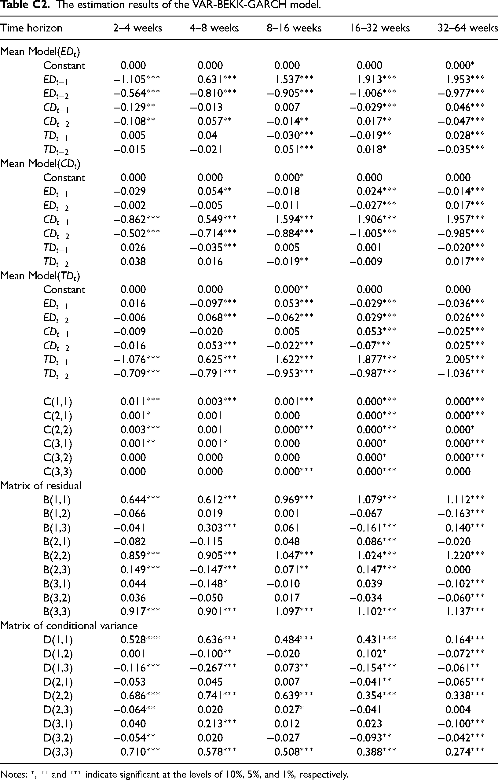
Appendix C

Table C2.

The estimation results of the VAR-BEKK-GARCH model.

Time horizon		2–4 weeks	4–8 weeks	8–16 weeks	16–32 weeks	32–64 weeks
Mean Model( $E D_{t}$ )
	Constant	0.000	0.000	0.000	0.000	0.000*
	$E D_{t - 1}$	−1.105***	0.631***	1.537***	1.913***	1.953***
	$E D_{t - 2}$	−0.564***	−0.810***	−0.905***	−1.006***	−0.977***
	$C D_{t - 1}$	−0.129**	−0.013	0.007	−0.029***	0.046***
	$C D_{t - 2}$	−0.108**	0.057**	−0.014**	0.017**	−0.047***
	$T D_{t - 1}$	0.005	0.04	−0.030***	−0.019**	0.028***
	$T D_{t - 2}$	−0.015	−0.021	0.051***	0.018*	−0.035***
Mean Model( $C D_{t}$ )
	Constant	0.000	0.000	0.000*	0.000	0.000
	$E D_{t - 1}$	−0.029	0.054**	−0.018	0.024***	−0.014***
	$E D_{t - 2}$	−0.002	−0.005	−0.011	−0.027***	0.017***
	$C D_{t - 1}$	−0.862***	0.549***	1.594***	1.906***	1.957***
	$C D_{t - 2}$	−0.502***	−0.714***	−0.884***	−1.005***	−0.985***
	$T D_{t - 1}$	0.026	−0.035***	0.005	0.001	−0.020***
	$T D_{t - 2}$	0.038	0.016	−0.019**	−0.009	0.017***
Mean Model( $T D_{t}$ )
	Constant	0.000	0.000	0.000**	0.000	0.000
	$E D_{t - 1}$	0.016	−0.097***	0.053***	−0.029***	−0.036***
	$E D_{t - 2}$	−0.006	0.068***	−0.062***	0.029***	0.026***
	$C D_{t - 1}$	−0.009	−0.020	0.005	0.053***	−0.025***
	$C D_{t - 2}$	−0.016	0.053***	−0.022***	−0.07***	0.025***
	$T D_{t - 1}$	−1.076***	0.625***	1.622***	1.877***	2.005***
	$T D_{t - 2}$	−0.709***	−0.791***	−0.953***	−0.987***	−1.036***

	C(1,1)	0.011***	0.003***	0.001***	0.000***	0.000***
	C(2,1)	0.001*	0.001	0.000	0.000***	0.000***
	C(2,2)	0.003***	0.001	0.000***	0.000***	0.000*
	C(3,1)	0.001**	0.001*	0.000	0.000*	0.000***
	C(3,2)	0.000	0.000	0.000	0.000*	0.000***
	C(3,3)	0.000	0.000	0.000***	0.000***	0.000
Matrix of residual
	B(1,1)	0.644***	0.612***	0.969***	1.079***	1.112***
	B(1,2)	−0.066	0.019	0.001	−0.067	−0.163***
	B(1,3)	−0.041	0.303***	0.061	−0.161***	0.140***
	B(2,1)	−0.082	−0.115	0.048	0.086***	−0.020
	B(2,2)	0.859***	0.905***	1.047***	1.024***	1.220***
	B(2,3)	0.149***	−0.147***	0.071**	0.147***	0.000
	B(3,1)	0.044	−0.148*	−0.010	0.039	−0.102***
	B(3,2)	0.036	−0.050	0.017	−0.034	−0.060***
	B(3,3)	0.917***	0.901***	1.097***	1.102***	1.137***
Matrix of conditional variance
	D(1,1)	0.528***	0.636***	0.484***	0.431***	0.164***
	D(1,2)	0.001	−0.100**	−0.020	0.102*	−0.072***
	D(1,3)	−0.116***	−0.267***	0.073**	−0.154***	−0.061**
	D(2,1)	−0.053	0.045	0.007	−0.041**	−0.065***
	D(2,2)	0.686***	0.741***	0.639***	0.354***	0.338***
	D(2,3)	−0.064**	0.020	0.027*	−0.041	0.004
	D(3,1)	0.040	0.213***	0.012	0.023	−0.100***
	D(3,2)	−0.054**	0.020	−0.027	−0.093**	−0.042***
	D(3,3)	0.710***	0.578***	0.508***	0.388***	0.274***

Notes: *, ** and *** indicate significant at the levels of 10%, 5%, and 1%, respectively.

References

Meckling

Allan

. The evolution of ideas in global climate policy. Nat Clim Chang 2020; 10: 434–438.

Linares

Santos

Ventosa

MJCP

. Coordination of carbon reduction and renewable energy support policies. Climate Policy 2008; 8: 377–394.

Schusser

Jaraitė

. Explaining the interplay of three markets: green certificates, carbon emissions and electricity. Energy Econ 2018; 71: 1–13.

Fischer

Preonas

. Combining policies for renewable energy: is the whole less than the sum of its parts? Resource for the Future Discussion Paper 2010.

Böhringer

Keller

Bortolamedi

, et al. Good things do not always come in threes: on the excess cost of overlapping regulation in EU climate policy. Energy Policy 2016; 94: 502–508.

Stavins

. Market-based environmental policies, public policies for environmental protection. London; New York: Routledge, 2010; 41–86.

Tinbergen

. On the theory of economic policy 1952 Chaps. 4 and 5.

Amundsen

Mortensen

. The Danish green certificate system: some simple analytical results. Energy Econ 2001; 23: 489–509.

Amundsen

Nese

. Integration of tradable green certificate markets: what can be expected? J Policy Model 2009; 31: 903–922.

10.

Böhringer

Rosendahl

. Green promotes the dirtiest: on the interaction between black and green quotas in energy markets. J Regul Econ 2010; 37: 316–325.

11.

Lee

B-H

Ahn

H-H

. Electricity industry restructuring revisited: the case of Korea. Energy Policy 2006; 34: 1115–1126.

12.

Acworth

de Oca

Boute

, et al. Emissions trading in regulated electricity markets. Climate Policy 2020; 20: 60–70.

13.

Moreno

García-Álvarez

. Analyzing the impact of fossil fuel import reliance on electricity prices: the case of the Iberian Electricity Market. Energy Environ 2017; 28: 687–705.

14.

Rathmann

. Do support systems for RES-E reduce EU-ETS-driven electricity prices? Energy Policy 2007; 35: 342–349.

15.

Jensen

Skytte

. Simultaneous attainment of energy goals by means of green certificates and emission permits. Energy Policy 2003; 31: 63–71.

16.

Engle

Ito

Lin

. Meteor showers or heat waves? Heteroskedastic intra-daily volatility in the foreign exchange market. Working Paper No. 2609. Cambridge: National Bureau of Economic Research, 1988.

17.

Lin

Engle

Ito

. Do bulls and bears move across borders? International transmission of stock returns and volatility. Rev Financ Stud 1994; 7: 507–538.

18.

Pal

Mitra

. Time-frequency dynamics of return spillover from crude oil to agricultural commodities. Appl Econ 2020; 52: 5426–5445.

19.

Engle

. Risk and volatility: econometric models and financial practice. Am Econ Rev 2004; 94: 405–420.

20.

Wang

Guo

. The dynamic spillover between carbon and energy markets: new evidence. Energy 2018; 149: 24–33.

21.

Coulon

Khazaei

Powell

. SMART-SREC: a stochastic model of the new jersey solar renewable energy certificate market. J Environ Econ Manage 2015; 73: 13–31.

22.

Han

Kordzakhia

Trück

. Volatility spillovers in Australian electricity markets. Energy Econ 2020; 90: 104782.

23.

Gong

Shi

, et al. Analyzing spillover effects between carbon and fossil energy markets from a time-varying perspective. Appl Energy 2021; 285: 116384.

24.

Ciarreta

Pizarro-Irizar

Zarraga

. Renewable energy regulation and structural breaks: an empirical analysis of Spanish electricity price volatility. Energy Econ 2020; 88: 104749.

25.

Hanif

Arreola Hernandez

Mensi

, et al. Nonlinear dependence and connectedness between clean/renewable energy sector equity and European emission allowance prices. Energy Econ 2021; 101: 105409.

26.

Reboredo

Rivera-Castro

. Wavelet-based evidence of the impact of oil prices on stock returns. Int Rev Econ Financ 2014; 29: 145–176.

27.

Fagiani

Hakvoort

. The role of regulatory uncertainty in certificate markets: a case study of the Swedish/Norwegian market. Energy Policy 2014; 65: 608–618.

28.

Ramsey

. Wavelets in economics and finance: past and future. Stud Nonlinear Dyn Econom 2002; 6: 3.

29.

Dai

Wang

Zha

, et al. Multi-scale dependence structure and risk contagion between oil, gold, and US exchange rate: a wavelet-based vine-copula approach. Energy Econ 2020; 88: 104774.

30.

Percival

Walden

. Wavelet methods for time series analysis. Cambridge: Cambridge University Press, 2000.

31.

Jiang

Yoon

S-M

. Dynamic co-movement between oil and stock markets in oil-importing and oil-exporting countries: two types of wavelet analysis. Energy Econ 2020; 90: 104835.

32.

Engle

Kroner

. Multivariate simultaneous generalized ARCH. Econ Theory 1995; 11: 122–150.

33.

Mensi

Hammoudeh

Nguyen

, et al. Dynamic spillovers among major energy and cereal commodity prices. Energy Econ 2014; 43: 225–243.

34.

Kwon

. Policy mix of renewable portfolio standards, feed-in tariffs, and auctions in South Korea: are three better than one? Util Policy 2020; 64: 101056.

35.

Park

Hong

. Korea׳S emission trading scheme and policy design issues to achieve market-efficiency and abatement targets. Energy Policy 2014; 75: 73–83.

36.

Chevallier

. A model of carbon price interactions with macroeconomic and energy dynamics. Energy Econ 2011; 33: 1295–1312.

37.

Hintermann

Peterson

Rickels

. Price and market behavior in phase II of the EU ETS: a review of the literature. Rev Environ Econ Policy 2020; 10: 108–128.

38.

Espey

. Renewables portfolio standard: a means for trade with electricity from renewable energy sources? Energy Policy 2001; 29: 557–566.

39.

Von Bremen

. Large-scale variability of weather dependent renewable energy sources, management of weather and climate risk in the energy industry. Dordrecht: Springer, 2010; 189–206.

40.

Kim

Chang

. Experience curve analysis on South Korean nuclear technology and comparative analysis with South Korean renewable technologies. Energy Policy 2012; 40: 361–373.

41.

Kwon

. Is the renewable portfolio standard an effective energy policy?: early evidence from South Korea. Util Policy 2015; 36: 46–51.

42.

Hellström

Lundgren

. Why do electricity prices jump? Empirical evidence from the nordic electricity market. Energy Econ 2012; 34: 1774–1781.

43.

Byrnes

Brown

Foster

, et al. Australian renewable energy policy: barriers and challenges. Renew Energy 2013; 60: 711–721.

44.

Pfenninger

Keirstead

. Renewables, nuclear, or fossil fuels? Scenarios for Great Britain’s power system considering costs, emissions and energy security. Appl Energy 2015; 152: 83–93.

45.

Tang

Zhang

. Oil price shocks and their short- and long-term effects on the Chinese economy. Energy Econ 2010; 32: S3–S14.

46.

Fouquet

. Path dependence in energy systems and economic development. Nat Energy 2016; 1: 1–5.

47.

Dong

Xue

. Demand response in China: regulations, pilot projects and recommendations – A review. Renew Sustain Energy Rev 2016; 59: 13–27.

48.

Tang

, et al. How to peak carbon emissions in China’s power sector: a regional perspective. Energy Policy 2018; 120: 365–381.

49.

Lin

Chen

. Does electricity price matter for innovation in renewable energy technologies in China? Energy Econ 2019; 78: 259–266.

The interplay of the carbon market,the tradable green certificate market,and electricity market in South Korea: Dynamic transmission and spillover effects

Abstract

Keywords

Introduction

Literature review

Methodology

VAR model construction

Multilevel time scales decomposition by discrete wavelet transform

VAR-BEKK-GARCH model

Data description

Model estimation and discussion

VAR model estimation and impulse response analysis

VAR model specification and diagnostics

Impulse response analysis

VAR-BEKK-GARCH model estimation at multi-time scales

Mean spillover at multi-time scales

Risk spillover at multi-time scales

Conclusion and policy implications

Footnotes

Declaration of conflicting interests

Funding

ORCID iD

Appendix A

Appendix B

Appendix C

References