One dimensional approach to predict the performance of high pressure multi-stage axial turbine considering air cooling and diffuser performance

Abstract

This paper provides an improved 1D mid-span program to quickly grasp the off-design characteristic of modern axial turbines. The improvements are mainly focused on cooling, diffuser and the calculation of choke condition. Disk cooling and blade cooling air mixing are considered in detail. A 1D diffuser model that considers the effects of area change, heat transfer, and friction is added so that a realistic boundary condition at the turbine outlet can be obtained. A choke routine that enables the assessment of choked flow up to limit load conditions is introduced to avoid the shortcoming that the calculation method fails to converge near or at the initial choking mass flow rate. Flexible modules for losses, deviation, and mixing models are built-in to increase the accuracy and versatility of the program. This work is of great value because few programs take cooling and diffuser into account in such detail when calculating turbine performance in the form of maps. The salient issues presented here deal first with the construction of the turbine performance prediction program. The validation of the code is first performed on public data for a five-stage low pressure turbine (LPT). The results show that the efficiency relative errors with the experimental value is in the range of −(0.11%−1.64%), which is within acceptable limits. Then, the performance of GE PG9351FA transonic axial turbine is estimated using this program. This industrial axial turbine is predicted for the first time in a form of turbine performance maps in open literature and the obtained performance map is very useful for the simulation of gas turbine.

Introduction

One-dimensional mid-span methods are widely used in the axial turbine preliminary design stage due to their speed and efficiency. And in the gas turbine conceptual design phase, the program using 1D method cannot merely provide the information needed in more detailed through-flow and Computational fluid dynamics (CFD) analyses but also can be integrated into the gas turbine simulation code to satisfy the needs of mastering performance of gas turbines in the full working operation range on the basis of very limited information. Therefore, although CFD is very popular nowadays, 1D method is still the focus and key point.

At present, some commercial software is available in the market for axial turbine performance analysis using 1D method. However, these commercial software have limitations when applying it into the gas turbine simulation: the codes are proprietary, and the secondary development based on user needs cannot be conducted.

With the development of the modern axial flow turbine technology, there is a strong need to develop, improve and verify cooling, deviation and loss models in 1D calculation. Many scholars conducted relevant studies, which are often packaged as a suite, such as object-oriented turbomachinery analysis code (OTAC), ¹ Denton’s series of codes, ² LUAX-T. ³ OTAC is the object-oriented turbomachinery analysis code developed by the National Aeronautics and Space Administration (NASA) Glenn Research Center. In Denton’s codes, the turbine performance analysis directly adopts the throughflow calculation. LUAX-T is a series of codes developed at Lund University and can perform 1D predictions considering cooling. However, problems and limitations still remain for studies on modern axial turbines with the feature of high pressure ratio, high inlet gas temperature and large cooling air flow.

The first problem is about the cooling. Modern day advanced axial turbines often use large amount of cooling, and the maximum nozzle temperature of the first stage has reached the level of 1800 K. Ignoring the effect of cooling on pressure ratio and temperature drop of mainstream leads to considerable errors. When cooling is considered, determining the coolant amount under variable working conditions and considering the mixing loss caused by cooling are relatively complex problems, which need effective treatment methods. However, in the open literature about the turbine performance prediction using 1D method, only LUAX-T considers cooling but the specific implementation and the adopted model are unavailable. ³

The second problem is about the diffuser. The diffuser has a strong influence on axial turbine performance, especially for industrial axial turbines. ⁴ Specifically, the optimal design (maximum efficiency) of axial turbines depends largely on the amount of kinetic energy that can be recovered from the last stage. ⁵ According to Bahamonde et al., ⁶ the discharge kinetic energy can be one of the main reasons of efficiency loss; its magnitude can reach the same order as the profile loss and secondary loss when the influence of the diffuser is disregarded during the preliminary design. Despite this condition, it is often neglected or just assumed a fraction of the outlet kinetic energy that is recovered during the preliminary design and analysis,^7–9 which may not be detailed and sufficiently accurate at today that the models have been so refined.

The third problem is about the calculation method of turbine performance analysis. Different from compressor normally working in non-choking condition, the turbine design point always falls within the choked region of the turbine characteristic curve. In this condition, traditional turbomachinery analysis programs, such as OTAC, calculate the pressure ratio distribution and total pressure ratio with a given mass flow rate, which may meet problems about convergence as the flow approach choking. Denton^1,3 proposed an innovative method that calculates the pressure ratio distribution and mass flow rate with a given total pressure ratio (the inlet mass flow is a derived quantity) to address this problem. However, the difficulty of this method lies in how to update the pressure ratio distribution reasonably. The inappropriate updating method of pressure leads to poor convergence. Denton’s program itself offers a solution. Subsequently, a simpler and more direct force style pressure solver is given by Came. ¹⁰ Joel claimed that this method has better convergence than Denton’s method. ¹¹ However, after the author’s verification, the Denton’s method is really difficult to converge, and the Came’s method still cannot obtain a correct result and fails to converge in the iterative calculation process although the iterative value produced by this method is closer to the correct answer. The probable reason is that finding the corresponding flow rate by constantly updating the pressure distribution and ensuring that the outlet pressure of each row is correct simultaneously are inherently difficult.

The fourth problem is about the choking. Different literature adopts different judgment methods, which are basically divided into two types: it is generally believed that the Mach number at the throat equals one is the criterion used when the turbine enters the initial choking condition. If so, the area of the throat needs to be known, and a new calculation station at the throat needs to be established. ³ However, loss models are insufficient to provide the chord-wise distribution, it can only estimate roughly that the fraction of loss that is generated before throat is 0.2–0.4 of the total loss in a cascade. ³ The other criterion is the outlet Mach number equals one. The mass flow rate at this time obviously does not reach the allowable mass flow constraint for an non isentropic flow. ¹² Such a judgment method deviates from the actual situation and is inaccurate.

From the above discussion, the methods in the literature are far from the requirement of establishing an accurate and complete calculation method for modern air-cooled turbine performance prediction. In this paper, based on the traditional method that calculating the pressure ratio distribution and total pressure ratio with given mass flow rate, the authors expand and improve it as follows.

First, cooling air mixing loss are considered row by row to reflect the fluid flow in the actual cooling. The number of calculation stations correspondingly increases from three (stator inlet, rotor inlet and rotor outlet) to seven by considering the injection of disk cooling air. Different mixing loss models are adopted under different conditions to ensure a good precision in the analysis. The loss due to the mixing of inlet cooling air is computed by using Hartsel’s mixing loss model ¹³ based on the energy equation and the momentum. The process of computing the mixing of the cooling air at the blade exit is conducted by using a more advanced 2D model based on control volume theory. Second, different from the previous simple way of dealing with it, a 1D diffuser modulation that can calculate the thermodynamic properties (including diffuser recovery factor) of diffuser outlet under different working conditions is added. This model is formulated as an implicit system of ordinary differential equations (ODEs) that consider the main features of the flow, such as the effects of area change, heat transfer, and friction. To the best of our knowledge, no model in the literature meets all these requirements; ¹⁴ Third, a choke routine that enable the assessment of choked flow up to limit load conditions is added into the program. This routine is introduced to enable the program to adapt to the condition that relative Mach number became supersonic, which is of particular importance for axial turbine performance characterization. Fourth, with regard to the judgement of the initial choking state, the criterion that the outlet Mach number is on the order of 0.94 ± 0.03 is selected. This not only solves the problem that the lack of loss model before throat but also ensures the relative accuracy of calculation. ³

This article is organized as follows: Section 1 presents the introduction. Section 2 contains a fairly detailed discussion about the deviation angle, cooling, loss, diffuser models used in this program. Section 3 provides the turbine performance prediction method. The method of determining the initial value of outlet pressure of every cascade is also provided, which is rarely mentioned in other articles. In Section 4, validation of this program is performed using a five-stage LPT. Then the performance of GE PG9351FA turbine, a three-stage highly loaded industrial turbine with the feature of high cooling air flow is predicted. Section 5 is the conclusion.

One-dimensional modeling

The major assumptions for 1D method are as follows:

The working fluid is regarded as a semi-perfect gas.

The turbine performance is represented by the aerothermodynamic parameters calculated at the mean radius.

The circumferential and spanwise parameters of the turbine are uniform and only change along the flow direction.

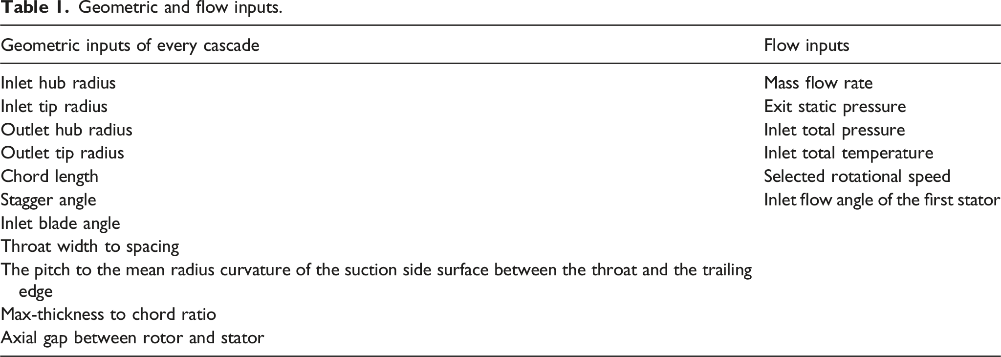
Inputs

Geometry and flow parameters are defined as inputs for turbine performance prediction program, as presented in Table 1.

Table 1.

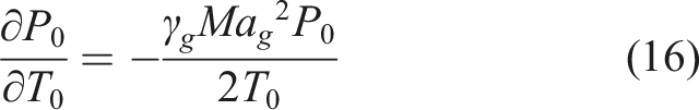
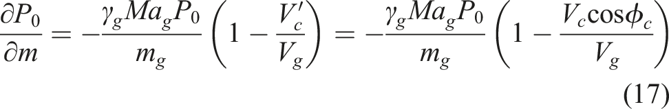
Geometric and flow inputs.

Geometric inputs of every cascade	Flow inputs
Inlet hub radius	Mass flow rate
Inlet tip radius	Exit static pressure
Outlet hub radius	Inlet total pressure
Outlet tip radius	Inlet total temperature
Chord length	Selected rotational speed
Stagger angle	Inlet flow angle of the first stator
Inlet blade angle
Throat width to spacing
The pitch to the mean radius curvature of the suction side surface between the throat and the trailing edge
Max-thickness to chord ratio
Axial gap between rotor and stator

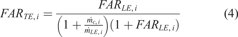
In this program, the full set of compositions of the main flow is calculated from fuel-to-air ratio (FAR). FAR is calculated at seven stations for each stage. The calculation method of thermodynamic properties is shown in the following section.

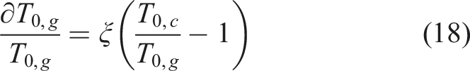
State properties

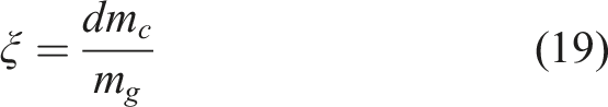
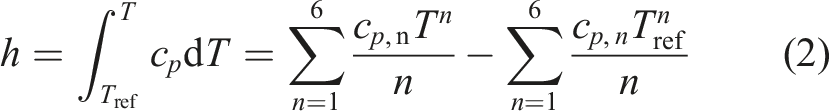
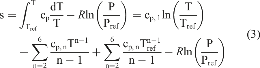
The calculation of state properties is based on the Gibbs-Dalton approach. ³ The Cp model used is the NASA SP-273 proposed by Gordon and McBride, ¹⁵ and the enthalpy and entropy are a function of Cp and temperature. The specific heat is expressed as a fifth-order polynomial: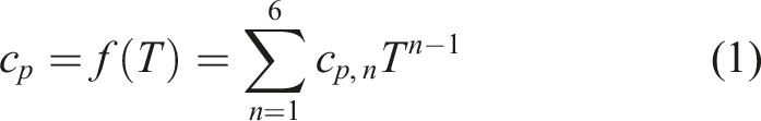

$c_p=f\left(T\right)={\displaystyle \sum }_{n=1}^6{c}_{p,n}{T}^{n-1}$

(1)

$h={\int }_{T_{\text{ref}}}^T{c}_p\mathrm{d}T={\displaystyle \sum }_{n=1}^6\frac{c_{p,\mathrm{n}}{T}^n}{n}-{\displaystyle \sum }_{n=1}^6\frac{c_{p,n}{T}_{\text{ref}}^n}{n}$

(2)

$\mathrm{s}={\int }_{{\mathrm{T}}_{\text{ref}}}^{\mathrm{T}}{\mathrm{c}}_{\mathrm{p}}\frac{\mathrm{d}\mathrm{T}}{\mathrm{T}}-\mathit{R}\ln \left(\frac{\mathrm{P}}{{\mathrm{P}}_{\mathrm{r}\mathrm{e}\mathrm{f}}}\right)={\mathrm{c}}_{\mathrm{p},1}\ln \left(\frac{\mathrm{T}}{{\mathrm{T}}_{\mathrm{r}\mathrm{e}\mathrm{f}}}\right)+{\displaystyle \sum }_{\mathrm{n}=2}^6\frac{{\mathrm{c}}_{\mathrm{p},\mathrm{n}}{\mathrm{T}}^{\mathrm{n}-1}}{\mathrm{n}-1}+{\displaystyle \sum }_{\mathrm{n}=2}^6\frac{{\mathrm{c}}_{\mathrm{p},\mathrm{n}}{\mathrm{T}}_{\mathrm{r}\mathrm{e}\mathrm{f}}^{\mathrm{n}-1}}{\mathrm{n}-1}-\mathit{R}\ln \left(\frac{\mathrm{P}}{{\mathrm{P}}_{\mathrm{r}\mathrm{e}\mathrm{f}}}\right)$

(3)

where $c_{p,n}$ is the empirical coefficient. In the above equation, the reference values P _ref and T _ref are set to 101.325 kPa and 273.15 K, respectively. Since the air and fuel composition are determined, the composition of the hot gas at every station can be calculated on the basis of the FAR: ³

$FA{R}_{TE,i}=\frac{FA{R}_{LE,i}}{\left(1+\frac{{\dot{m}}_{c,i}}{{\dot{m}}_{LE,i}}\right)\left(1+FA{R}_{LE,i}\right)}$

(4)

The ratio of disk cooling to the total cooling of every stage is given as input data.

Empirical models

The cascade outlet flow parameters are mainly obtained on the basis of loss, deviation, cooling and choke models. And the accuracy of these models directly determines whether the final calculation result is accurate or not. ¹⁶

Deviation angle model

The deviation angle is an essential and important parameter in turbine performance prediction. It directly determines the outlet flow angle of the cascade, and hence the velocity triangle and aerodynamic performance. Many deviation angle models have been proposed. These models fall into two main categories.

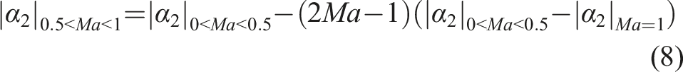
The first category is based on Ainley’s model. ¹⁷ Ainley proposed an empirical correlation based on a large number of turbine tests. The outlet flow angle at low Mach number remains constant while the flow angle at high Mach number is only a function of the Mach number. In order to consider the influence of secondary flow and correct the effect of tip clearance on flow angle, Traupel and Hubert ¹⁸ then introduced the corresponding modified correlations.

The second category is based on Carter’s model. ¹⁹ Carter and Hughes estimated deviation angle as a function of blade stagger angle, blade camber, and the solidity. This deviation model is originally used for compressors but can also be applied to turbines with specific settings. But, for modern turbine blades, this model overpredicts the deviation largely. It is then modified by including flow turning, stagger angle and maximum thickness-to-chord ratio, which is regarded as additional and more influential correlating parameters according to Islam and Sjolander. ²⁰ The obtained correlation appears more successful than Carter’s correlation. ¹⁹ Subsequently, the influence of Reynolds number was added to the correlation, and the form of the correlating function was revised by zhu and Sjolander. ²¹ The range of flow and geometric parameters for which it is applicable was extended. But the accuracy of the series of modified Carter’s model mentioned above is relatively insufficient for practical calculation of the two cases in the section 4.

Shchegliaev ²² proposed a simple deviation angle model suitable for the condition that the outlet Mach number less than 1:

$\sin {\alpha }_2=m\cdot \sin {\alpha }_{gau}$

(5)

where m≈1 for modern aerodynamically efficient profiles, which means that the outlet flow angle is equal to the gauge angle, cos⁻¹(O/S). ²²

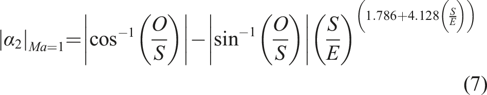
In order to accurately calculate the deviation angle of transonic flow, Mamaev^23,24 proposed a model for the flow velocity at 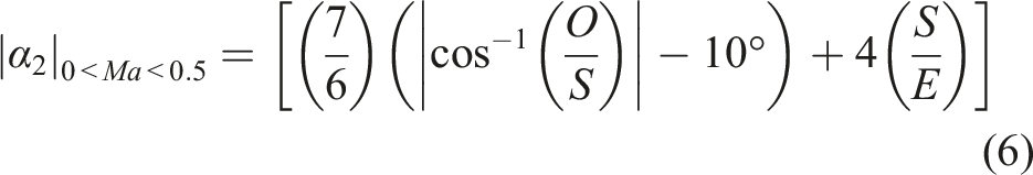${\lambda }_2$ ≈0.9–1.1. This model is complicated and uses the theorem of angular momentum and control volume analysis at the throat and cascade outlet. ¹¹ Many parameters, such as, the kinetic energy loss coefficient, functions p, $\pi$ , and y, are used to calculate the limiting velocity so that the flow can be determined whether it is sonic or not. However, these nonlinear equations are so complex that the fsolve function (used to solve nonlinear systems of equations in MATLAB) difficult to converge. ²³ According to the author’s experience, it may take several hours to converge. On this basis, even though Mamaev’s method is detailed enough, it may not be a good choice. After verification, Ainley’s model^17,25 works well in the case of GE PG9351FA, and its detailed model is given as follows:for 0.0<Ma<0.5,

${\left|{\alpha }_2\right|}_{0<Ma<0.5}=\left[\left(\frac{7}{6}\right)\left(\left|{\cos }^{-1}\left(\frac{O}{S}\right)\right|-10°\right)+4\left(\frac{S}{E}\right)\right]$

(6)

for Ma=1,

${\left|{\alpha }_2\right|}_{Ma=1}=\left|{\cos }^{-1}\left(\frac{O}{S}\right)\right|-\left|{\sin }^{-1}\left(\frac{O}{S}\right)\right|{\left(\frac{S}{E}\right)}^{\left(1.786+4.128\left(\frac{S}{E}\right)\right)}$

(7)

for 0.5<Ma<1,

${\left|{\alpha }_2\right|}_{0.5<Ma<1}={\left|{\alpha }_2\right|}_{0<Ma<0.5}-\left(2Ma-1\right)\left({\left|{\alpha }_2\right|}_{0<Ma<0.5}-{\left|{\alpha }_2\right|}_{Ma=1}\right)$

(8)

where E is the radius of curvature of blade convex surface downstream of throat.

Considering the effect of causing over and under turning due to secondary flow and tip clearance for unshrouded blades, the Ainley’s model ¹⁷ is corrected according to Traupel: ¹⁸

${\alpha }_{corr}={\alpha }_2-70.5\frac{clr}{c}\frac{r_{hub}}{r_{Euler}}+0.714\frac{S}{H}$

(9)

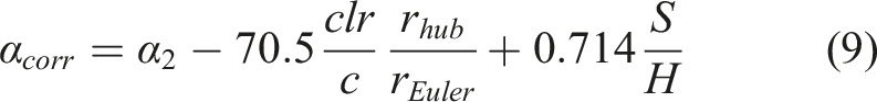
The Euler radius is defined as follows: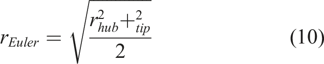

$r_{Euler}=\sqrt{\frac{r_{hub}^2{+}_{tip}^2}{2}}$

(10)

where r _Euler splits an annulus area into two equally sized annuli.

But for five-stage LPT, the convergence of the program worsens after using the deviation angle model of Ainley. The exact reason is unclear. Hence, the Shchegliaev’s deviation angle model ²² is used, indicating that the influence of off-design conditions on the deviation angle is ignored. In addition, some of the signs from the original correlations are modified to comply with the angle convention used in this work.

Cooling model

For modern industrial gas turbines, cooling air accounts for a large percentage of the compressor inlet flow, reaching approximately to 20%. If the influence of this part of cooling air is omitted during part-load operation, a large error or divergence appears. In the calculation of the turbine part-load performance prediction, the cooling air cannot be determined the same way as in the design program that the coolant mass flow rate of each blade row is calculated on the basis of the specified design blade temperature and the cooling parameters. Instead, the turbine always passively receives the cooling air conveyed from the extraction of the compressor.^26,27 (Although over-cooling, it is in line with the actual operation law). ²⁸ Therefore, the following formulation is usually used to determine the cold air amount: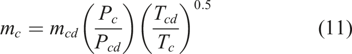

$m_c=m_{cd}\left(\frac{P_c}{P_{cd}}\right){\left(\frac{T_{cd}}{T_c}\right)}^{0.5}$

(11)

The coolant flow rate is modified in accordance with the temperature and pressure at the bleeding point of the compressor under the corresponding off-design conditions. The correlation is mainly derived from Freuger’s formulation: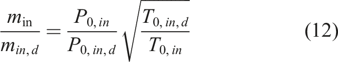

$\frac{m_{\text{in}}}{m_{in,d}}=\frac{P_{0,in}}{P_{0,in,d}}\sqrt{\frac{T_{0,in,d}}{T_{0,in}}}$

(12)

where P _0,in and T _0,in are the total (stagnation) temperature and pressure of the main gas at the inlet of the turbine, respectively.

According to the flow matching principle, the compressor can use the above mentioned correlation to estimate the bleeding air mass flow rate. However, the common working point of the compressor and the turbine also cannot be determined when the turbine characteristic curve is unknown, so the corresponding turbine inlet pressure and temperature cannot be known and this method cannot be used. But fortunately, based on the prior experience, ²⁹ the relative amount of cooling air at each stage of the turbine (the ratio of the cooling air to the inlet flow of the turbine) can almost be regarded as constant under variable working conditions. Therefore, the cooling air amount at each stage can be determined according to the following correlation when calculating the turbine map: ³⁰

$m_c=\frac{m_{cd}}{m_{g,stage,d}}{m}_{g,stage}$

(13)

where $m_c$ is the cooling air of a turbine stage; $m_{g,\text{stage}}$ is the gas mass flow at the inlet of a turbine stage.

This method can effectively determine the coolant amount at part-load conditions. In this model, the calculation of cooling air of each stage is specific to the stator and rotor, that is, considered row by row. Surely, the mixing of the cooling with the mainstream that causes the cascade aerodynamic loss is not ignored and discussed in the next section.

Mixing loss model

The existence of purge flow through the stator–rotor cavity, film cooling, and cooling air injection at the trailing edge all leads to the mixing of the cooling air with the main flow, which inevitably causing the cascade aerodynamic loss. Two models that are essentially based on the energy equation and the momentum equation are used in this paper to calculate this aerodynamic loss. Both of the models use the same assumption that the mixing is performed during constant static pressure and area.

Hartsel’s mixing loss model

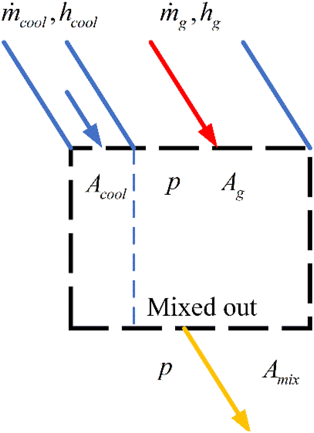
This widely used model mainly uses Shapiro’s influence coefficients method. ³¹ The 1D slot for the coolant-mainstream mixing is shown in Figure 1.

Figure 1.

The coolant-mainstream mixing.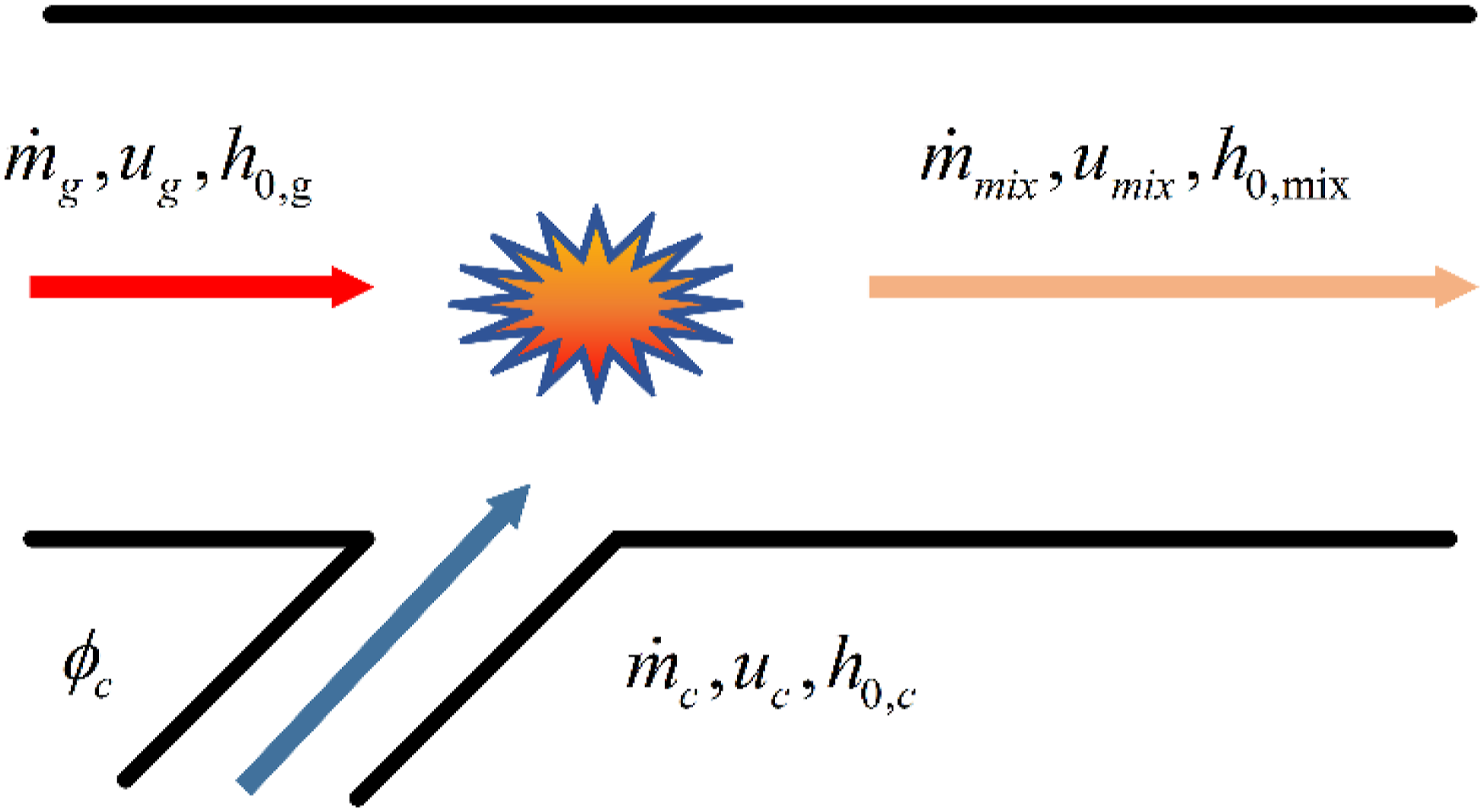

The Hartsel’s mixing loss model ¹³ is shown as:

$d{P}_0=\left(\frac{\partial P_0}{\partial A}\right)dA+\left(\frac{\partial P_0}{\partial T_0}\right)d{P}_0+\left(\frac{\partial P_0}{\partial m}\right)dm$

(14)

where

$\frac{\partial P_0}{\partial A}=0$

(15)

$\frac{\partial P_0}{\partial T_0}=-\frac{{\gamma }_{g}M{a_g}^2{P}_0}{2T_0}$

(16)

$\frac{\partial P_0}{\partial m}=-\frac{{\gamma }_{g}Ma{}_g{P}_0}{m_g}\left(1-\frac{V_c^{\prime }}{V_g}\right)=-\frac{{\gamma }_{g}Ma{}_g{P}_0}{m_g}\left(1-\frac{V_c\cos {\varphi }_c}{V_g}\right)$

(17)

$\frac{\partial T_{0,g}}{T_{0,g}}=\xi \left(\frac{T_{0,c}}{T_{0,g}}-1\right)$

(18)

$\xi =\frac{d{m}_c}{m_g}$

(19)

where $\xi$ is the ratio of coolant-to-mainstream mass flow rates, and ${\varphi }_c$ is the angle of coolant injection measured from local mainstream direction. Equations (15–18) are derived from the momentum equation and energy equation. Rearranging gives the equation below:

$\frac{d{P}_0}{P_{0,g}}=-\frac{\gamma }{2}\cdot M{a_g}^2\cdot \xi \cdot \left(1+\frac{T_{0,c}}{T_{0,g}}-2\frac{W_c}{W_g}\cos {\varphi }_c\right)$

(20)

$dS=-R\log \left(1-{\left(\frac{dP}{P_{0,g}}\right)}_0\right)$

(21)

where ${\mathit{cos}\varphi }_c$ is difficult to determine in the preliminary design stage, then the equation is simplified by assuming an injection of the cooling air normal to the streamline according to Olsson ³² when calculating the purge flow losses at the turbine inlet.

Trailing edge injection mixing model

This model is a 2D trailing edge injection mixing, which is described in detail in literature. ³² Different from Hartsel’s model, ¹³ the coolant flow is in the same direction with the main flow. Trailing edge loss is calculated in terms of the total enthalpy and the static pressure of the mixed flow. The calculation process needs to be computed in an iterative manner because the pressure after mixing is unknown. This model is based on the constant area and static pressure, which can be seen in Figure 2.

Figure 2.

Mixing at the trailing edge. ³³

Loss model

The internal flow loss inside the cascade is huge and has a great influence on the prediction of turbine performance, which cannot be ignored. Many of the prediction models such as Soderberg, ³⁴ Ainley and Mathieson, ¹⁷ Craig and Cox, ³⁵ Zehner, ³⁶ Moustapha and Benner, ³⁷ have been developed theoretically and experimentally. The loss models under off-design condition are all modified on the basis of the loss models at design points. And the difference between the loss under variable condition and the loss at design condition is mainly reflected in the incidence loss.

Soderberg’s model ³⁴ does not take the inlet boundary layer, the blade geometry and tip clearance into consideration, which is regarded as a big deficit. Zehner’s profile incidence loss model ³⁶ is mainly used for the calculation far from the design point. Ainley and Mathieson ¹⁷ proposed a method for calculating turbine losses under part load conditions. Subsequently, this method was modified by Dunham and Came, ³⁸ Kacker and Okapuu. ³⁹ The modifications mainly focus on profile loss, secondary loss, and clearance loss at design condition. Moustapha and Kacker ³⁷ improved the calculation method of profile and secondary incidence loss under off-design conditions, and considered that incidence loss is a function of blade leading edge diameter, spacing, and flow angle at the inlet and outlet, which is called AMDCKOMK in the remaining part of this paper. ³⁷ Benner and Sjolander ⁴⁰ proposed a more reasonable blade profile loss prediction model based on the work of Moustapha, ³⁷ considered not only the influence of the leading edge diameter but also the wedge angle. Craig and Cox gave the secondary losses that correlate to more parameters. The secondary loss in Craig and Cox model ³⁵ is calculated with a linear function of basic secondary loss, aspect ratio, and the factors of Reynolds number. The basic secondary loss is associated with blade solidity, ratio of inlet and outlet flow velocities, and the lift parameter, which is a function of the inlet and outlet flow angles.

After testing the aboved models, the loss model given by Craig and Cox ³⁵ has been used in the performance prediction considering the convergence and applicability. The incidence loss predicted by Craig and Cox reflects in profile loss. The incidence correction factor $N_{\text{pi}}$ is used to consider the profile loss that varies with the incidence. The variation of the loss coefficient of incidence $N_{\text{pi}}$ with the incidence ratio is shown in Figure 3, and the minimum incidence is given by Equation (22).

$i_{\min }=\frac{i_{stall}^{+}+F_i{i}_{stall}^{-}}{1+F_i}$

(22)

The stall incidence $i_{\text{stall}}$ is defined as the incidence in which the profile loss is twice the minimum value. $i_{\text{stall}}^{+}$ is the positive stalling incidence, whereas $i_{\text{stall}}^{\_}$ is the negative stalling incidence. F _i is the incidence range ratio. These incidence parameters are calculated by using the following equations:when $\alpha$ ≤90°,

$i_{stall}^{+}={\left(i_{stall}^{+}\right)}_{basic}+{\left(i_{stall}^{+}\right)}_{s/b}+{\left(i_{stall}^{+}\right)}_{CR}$

(23)

$i_{stall}^{-}={\left(i_{stall}^{-}\right)}_{basic}+{\left(i_{stall}^{-}\right)}_{s/b}$

(24)

when $\alpha$ >90°,

$i_{stall}^{+}={\left(i_{stall}^{+}\right)}_{basic}+\left(1-\frac{\alpha -90}{90-{\sin }^{-1}\left(o/s\right)}\right)\left[{\left(i_{stall}^{+}\right)}_{s/b}+{\left(i_{stall}^{+}\right)}_{CR}\right]$

(25)

$i_{stall}^{-}={\left(i_{stall}^{-}\right)}_{basic}+\left(1-\frac{\alpha -90}{90-{\sin }^{-1}\left(o/s\right)}\right){\left(i_{stall}^{-}\right)}_{s/b}$

(26)

where basic negative stalling incidence ${\left(i_{\text{stall}}^{+}\right)}_{\text{basic}}$ , basic negative stalling incidence ${\left(i_{\text{stall}}^{-}\right)}_{\text{basic}}$ , ${\left(i_{\text{stall}}^{+}\right)}_{s/b}$ and ${\left(i_{\text{stall}}^{+}\right)}_{\text{CR}}$ are incidence corrections for positive stalling incidence considering the pitch to backbone length ratio and blade contraction ratio, respectively. ${\left(i_{\text{stall}}^{-}\right)}_{s/b}$ is the incidence correction for negative stalling incidence considering the pitch to backbone length ratio. All of them are calculated by empirical formulation summarized from two-dimensional cascade experimental data, $\alpha$ is the blade inlet angle. ³⁵

Figure 3.

Incidence loss. ³⁵

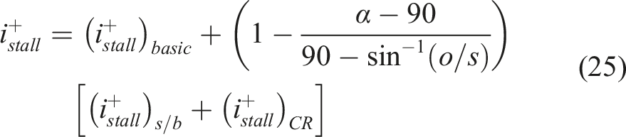
The correlation of secondary loss and tip clearance loss is the same with design condition. For the five-stage LPT, the efficiency predicted by Craig and Cox loss model ³⁵ is approximately 4.7% greater than the reference data. This model is an empirical formula directly summarized on the basis of 2D or 3D cascade data. It is inferred that the reason for this big deviation is that the model overestimates the influence of the flow angle at the inlet and outlet of the cascade among the factors affecting the profile loss. Therefore, in order to make the model suitable for code validation cases, an empirical manual increment (which remains constant at each rotational speed) is suggested to add to the original model in this paper. Of course, this kind of modification may too straightforward, and the Craig and Cox model needs to be improved from the flow mechanism to make it conform to the actual situation of flows inside the cascade, which will be discussed in future studies.

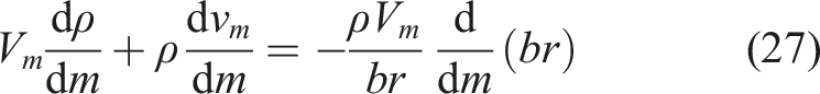
Diffuser model

The diffuser is frequently adopted to recover the discharge kinetic energy and increase the total-to-static isentropic efficiency. In this paper, the diffuser model is mainly derived from the transport equations for mass, meridional and tangential momentum, and energy in an annular channel. The system of ODEs are as follows:

$V_m\frac{\mathrm{d}\rho }{\mathrm{d}m}+\rho \frac{\mathrm{d}{v}_m}{\mathrm{d}m}=-\frac{\rho V_m}{br}\frac{\mathrm{d}}{\mathrm{d}m}\left(br\right)$

(27)

$\rho V_m\frac{\mathrm{d}{v}_m}{\mathrm{d}m}+\frac{\mathrm{d}p}{\mathrm{d}m}=\frac{\rho V_{\theta }^2}{r}\sin \left(\varphi \right)-\frac{2{\tau }_{\mathrm{w}}}{b}\cos \left(\alpha \right)$

(28)

$\rho v_m\frac{\mathrm{d}{V}_{\theta }}{\mathrm{d}m}=-\frac{\rho V_{\theta }{V}_m}{r}\sin \left(\varphi \right)-\frac{2{\tau }_{\mathrm{w}}}{b}\sin \left(\alpha \right)$

(29)

$\rho V_m\frac{\mathrm{d}P}{\mathrm{d}m}-\rho V_m{a}^2\frac{\mathrm{d}\rho }{\mathrm{d}m}=\frac{2\left({\tau }_{\mathrm{w}}V+{\dot{q}}_{\mathrm{w}}\right)}{b{\left(\frac{\partial e}{\partial P}\right)}_{\rho }}$

(30)

where $\varphi$ is the mean wall cant angle or angle between the radial and meridional directions, b is the height of the channel measured normal to the meridional direction, r is the radius of the annular diffuser. The corresponding cylindrical coordinate system with axial, radial, and axes is shown in Figure 4. The geometry of the diffuser can be seen in Figure 5.

Figure 4.

Differential control volume used to derive the diffuser governing equations. ¹⁴

Figure 5.

Axial-radial view of connection of the diffuser model. ¹⁴

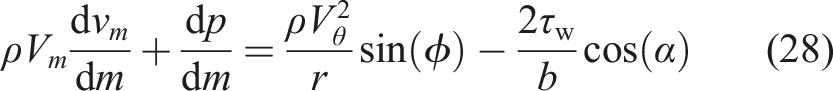
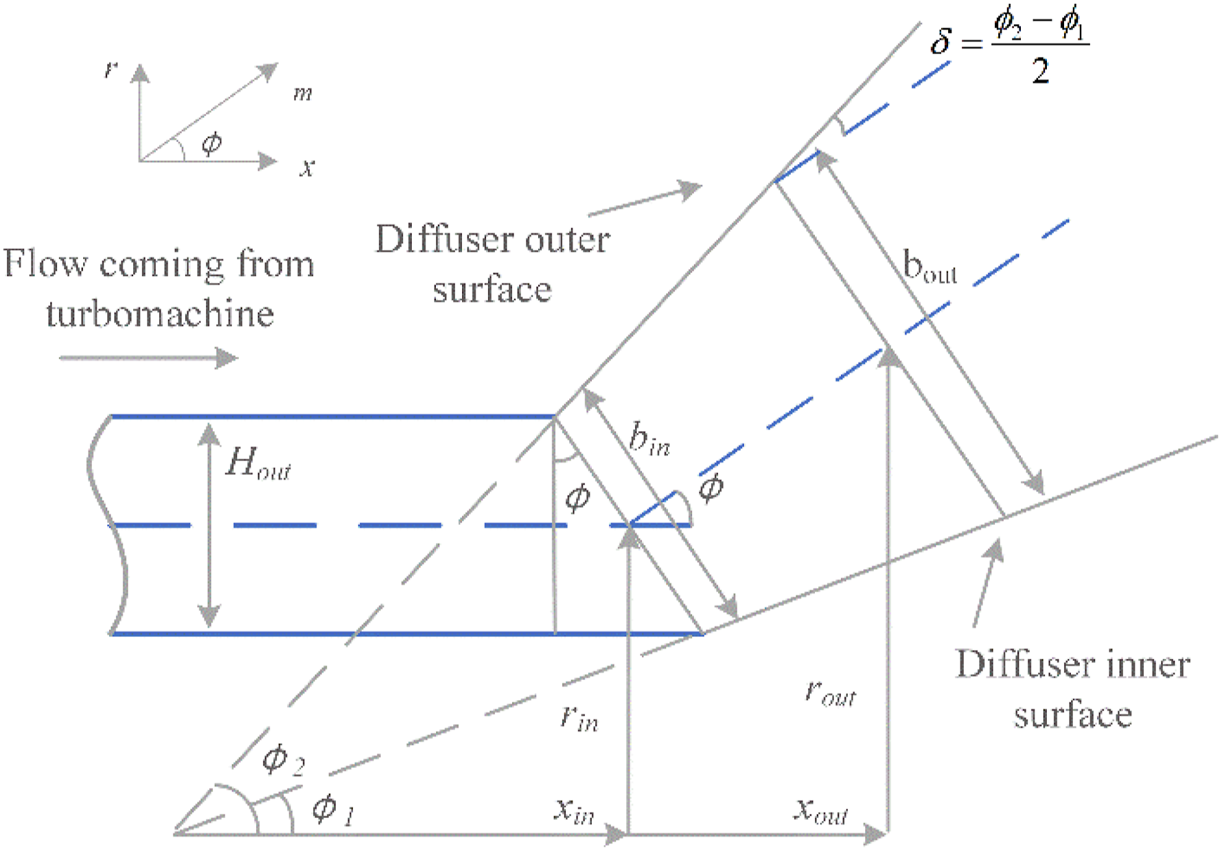
The viscous stress at the wall ${\tau }_w$ is computed on the basis of the skin coefficient C _f as given below:

${\tau }_{\mathrm{w}}=C_f\frac{\rho V^2}{2}$

(31)

On the basis of Reynolds analogy, the heat flux ${\dot{q}}_w$ is proportional to the temperature difference between the wall and the fluid:

${\dot{q}}_{\mathrm{w}}=\frac{\rho V{c}_p}{2}{C}_f\left(T_w-T_0\right)$

(32)

The form of the model, which is taken in the program, is as follows:

$\begin{array}{l}{\left[\mathrm{T},\mathrm{P},\mathrm{\rho },\mathrm{s},\mathrm{\eta },\mathrm{h},\mathrm{R}\mathrm{E}\mathrm{C}\mathrm{O}\mathrm{V}\dots \right]}_{\mathrm{o}\mathrm{u}\mathrm{t}}=\mathrm{f}\\ \left(\mathit{c}\mathit{a}\mathit{n}\mathit{t}\_\mathit{a}\mathit{n}\mathit{g}\mathit{l}\mathit{e},\mathit{div},\mathit{A}\mathit{R},{\mathit{C}}_{\mathrm{f}},{\mathrm{\rho }}_{\mathrm{i}\mathrm{n}},{\mathit{P}}_{\mathrm{i}\mathrm{n}},{\mathit{P}}_{0,\mathrm{i}\mathrm{n}},{\mathit{s}}_{\mathrm{i}\mathrm{n}},{\mathit{V}}_{\mathrm{m},\mathrm{i}\mathrm{n}},{\mathit{U}}_{\mathrm{m},\mathrm{i}\mathrm{n}},\mathit{F}\mathit{A}{\mathit{R}}_{\mathrm{i}\mathrm{n}},{\mathit{r}}_{\mathrm{m},\mathrm{i}\mathrm{n}},{\mathit{H}}_{\mathrm{i}\mathrm{n}}\right)\end{array}$

(33)

where div is the diffuser divergence semi-angle, AR is the diffuser area ratio, C _f is the skin friction coefficient and RECOV is the recovery factor. In this model, the diffuser geometry is fixed once the first four variables are determined. Then, given the inlet boundary conditions and these four geometrical parameters, the outlet parameters can be obtained. These four geometrical parameters are all obtained from the calculation results of the turbine design program.

Isentropic efficiency

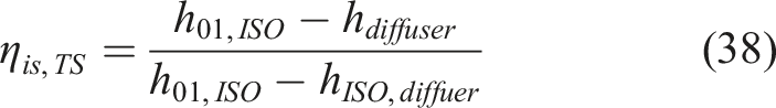
The stage isentropic efficiency is defined as the ratio between the real enthalpy difference and the isentropic enthalpy difference due to the expansion. However, this value will probably be greater than one once the turbine is cooled. ³ Therefore, the ISO-condition is introduced, indicating that the enthalpy change caused by cooling is subtracted at the beginning of the stage. The new ISO-condition inlet enthalpy can be calculated as: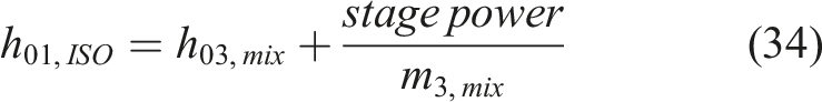

$h_{01,ISO}=h_{03,mix}+\frac{stage power}{m_{3,mix}}$

(34)

Correspondingly, the total-to-total stage isentropic efficiency is defined as: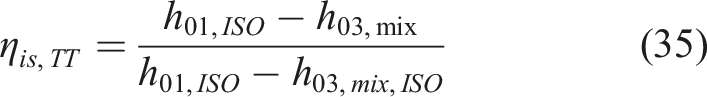

${\eta }_{is,TT}=\frac{h_{01,ISO}-h_{03,\text{mix}}}{h_{01,ISO}-h_{03,mix,ISO}}$

(35)

The above equation is applicable to the case where the outlet kinetic energy is recovered. When the outlet kinetic energy is lost, the isentropic total-to-static definition is more appropriate: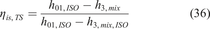

${\eta }_{is,TS}=\frac{h_{01,ISO}-h_{3,mix}}{h_{01,ISO}-h_{3,mix,ISO}}$

(36)

For the whole turbine machine with diffuser, the corresponding isentropic total-to-total and total-to-static definitions are as follows: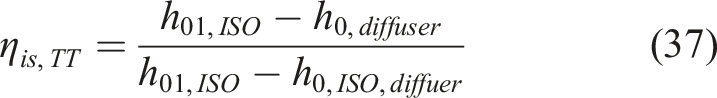

${\eta }_{is,TT}=\frac{h_{01,ISO}-h_{0,diffuser}}{h_{01,ISO}-h_{0,ISO,diffuer}}$

(37)

${\eta }_{is,TS}=\frac{h_{01,ISO}-h_{diffuser}}{h_{01,ISO}-h_{ISO,diffuer}}$

(38)

The thermal efficiency, also known as internal efficiency, is a relation between the stage power produced and the ideal work output from the stage. The stage power is the total power produced in the stage included the pumping power, which pump the cooling air from its inlet radius to the mean radius: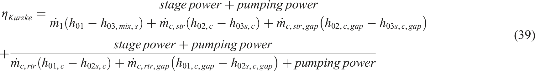

$\begin{array}{l}{\eta }_{Kurzke}=\frac{stage power+pumping power}{{\dot{m}}_1\left(h_{01}-h_{03,mix,s}\right)+{\dot{m}}_{c,str}\left(h_{02,c}-h_{03s,c}\right)+{\dot{m}}_{c,str,gap}\left(h_{02,c,gap}-h_{03s,c,gap}\right)}\\ +\frac{stage power+pumping power}{{\dot{m}}_{c,rtr}\left(h_{01,c}-h_{02s,c}\right)+{\dot{m}}_{c,rtr,gap}\left(h_{01,c,gap}-h_{02s,c,gap}\right)+pumping power}\end{array}$

(39)

The stage total pressure ratio is expressed as follows:

$\mathit{PR}=P_{01}/P_{03,mix}$

(40)

Considering the effect of the diffuser, the definition of the total pressure ratio of the turbine is expressed as:

$\mathit{PR}=P_{0,in}/P_{0,diffuser}$

(41)

where $P_{0,\text{in}}$ is the turbine inlet pressure before disk cooling air mixing. This definition of total pressure ratio is also used in the characteristic curve.

Program design

Turbine performance analysis methods are basically divided into two categories. The first category is based on a given mass flow rate and other input parameters,^17,41 which are similar with the compressor analysis method, which has no outlet pressure constraints, that is, sequential calculation stage by stage. Yet, Hendricks ¹ pointed out that this method may meet problems about convergence at conditions near and after choke because choke is likely to occur in the last few stages for the turbine at off-design conditions, so the change of pressure ratio with mass flow rate is effectively infinite. In this circumstance, finding the correct pressure ratio just by making small adjustments to the inlet flow rate is almost impossible. Even small adjustments to the inlet flow rate may cause the last stage to change its predicted performance. New solutions need to be explored from the initial choking to the limit loading condition.

The second category is based on a given outlet pressure (or pressure ratio) and other inlet parameters.^1,3 The main idea behind this method is that a certain pressure distribution yields a specific mass flow. This method can be divided into backward and forward. In the backward method, an inlet mass flow is assumed at first, and then the performance parameters at the inlet of every cascade are calculated from the last row based on the known turbine outlet pressure. The inlet parameters of the first stage calculated at last may not be the expected one. Thus, updating the mass flow and iterate are necessary until convergence is achieved.

The forward method, as the name suggests, starts from the first stage. This method can be performed in many different means, such as when calculating the outlet parameters of the cascade, updating the outlet pressure to ensure that the mass flow at inlet blade row equals the outlet flow. Since the outlet pressure of the last blade row has been determined, the mass flow rate of the last row has been determined and must be different from that of the previous rows. The last and most important step is to adjust the assumed mass flow, which is set as input, until these two mass flow rates are unified. This method can avoid the problem that pressure iteration is difficult to convergence, but it has certain requirements for the initial mass flow rate and outlet pressure distribution and it is easy to appear non-convergence under the condition of low pressure ratio.

Another way to perform is by retaining the cascade outlet mass flow, which calculated on the basis of the assumed outlet pressure distribution. That means the continuity equation at the blade trailing edge is abandoned, that is to say, the inlet mass flow rate and outlet mass flow in one blade are not consistent. According to the continuity of flow, the next rotor inlet flow is determined in accordance with the incorrect outlet flow of the last row. Then, the flow at the first trailing edge is selected as the target flow. After all the blade rows are calculated, the pressure distribution and target flow of the turbine are updated to find a new pressure distribution that balances the calculated mass flows at all cascades. The initial distribution of the outlet pressure can be assumed linear or obtained by informed guesswork. Setting a very accurate initial value may be unnecessary because a relatively stable and precise value will be calculated in the following iterations. This method can deal with both subsonic and supersonic flows. ² And there is no need to divide the calculation into two sections (choke and non-choke condition).

Even though there are so many turbine performance analysis methods, the stage calculation method is almost unchanged, and the basic principles and formulas are the same. Therefore, implementing all these methods is not needed. In the view of the stability and convergence of the program, this paper adopts the method with given mass flow. A flow diagram, which is shown in Figure 7, displays the architecture of the sequential performance prediction calculation program with given mass flow rate under non-choking conditions in detail.

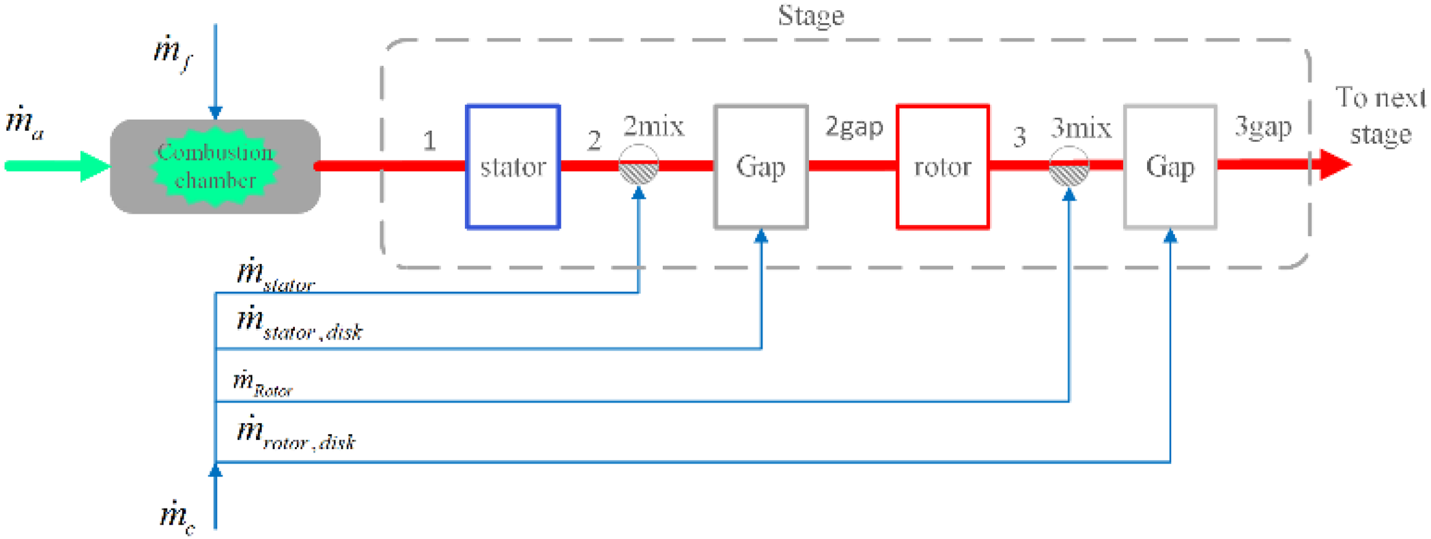
Figure 6 shows the meridional projection of stage computing station. This 1D compressible flow program with fast convergence basically estimates the representative meanline velocity diagrams located at seven axial stations for each stage, and when the overall thermal parameters at the stage outlet is calculated, this process repeats for each stage until the cumulative turbine performance is calculated. The specific calculation steps for cooling air mixing are as follows: the inlet flow of the stator blade is assumed to be the main airflow before mixing with the cooling air of the stator ${\dot{m}}_{\text{stator}}$ . Because the disk is also one of the turbine's high temperature components, the cooling air ${\dot{m}}_{\text{stator},\text{disk}}$ cannot be ignored. The gas mixed with the two cooling air flows accelerates in the rotor blade, and the rotor cooling air ${\dot{m}}_{\text{rotor}}$ mixes with the main gas at the outlet of the rotor blade. The disk cooling air ${\dot{m}}_{\text{rotor},\text{disk}}$ is mixed with the main gas at the inlet of the next stator. It is obvious that the rotor cooling air does not participate in the expansion work of the rotor blade at this stage.

Figure 6.

Schematic of turbine calculation station in a stage. ³³

During the process of program debugging, some points must to be noted. For example, the relative velocity w ₃ is calculated by using the constant rothalpy assumption and needs to be obtained by taking the square root:

$w_3=\sqrt{2\cdot \left(h_{2,gap}-h_3+1/2w_{2,gap}^2+1/2\left(U_3^2-U_{2,gap}^2\right)\right)}$

(42)

In the intermediate iterative calculation, the value of w ₃ sometimes dips below 0. The probable reason may be that the mass flow rate error is extremely large in the last iteration. When the stator or rotor mass flow loop (in Figure 7) starts again, the new value of the outlet pressure of the blade is inappropriate and leads to the calculated negative velocity w ₃ . An effective solution is to force the value to 0 to ensure the running of the program.

Figure 7.

Main architecture of the program at non-choking condition.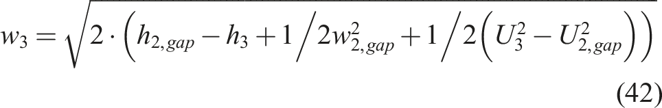

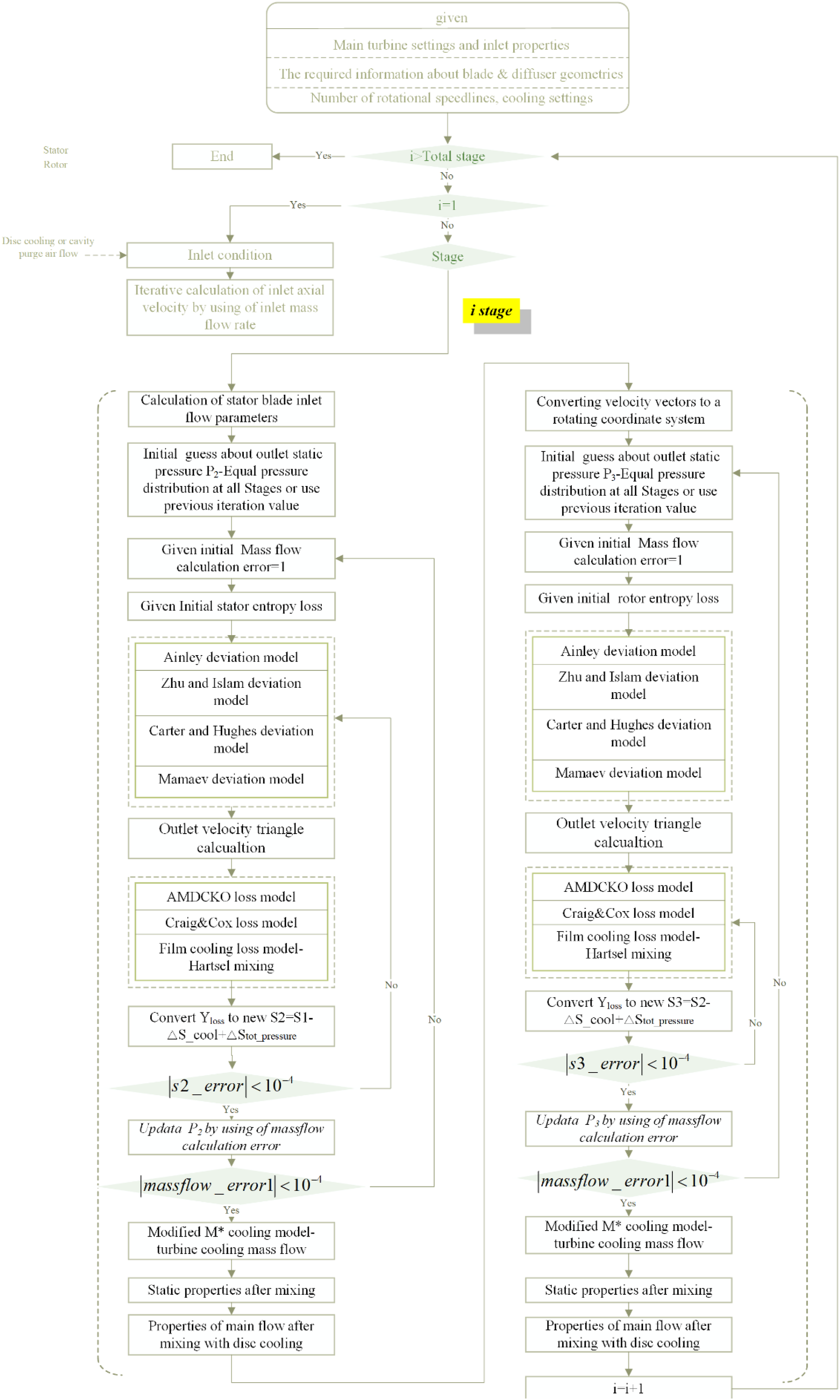
As for the setting of the initial value of outlet pressure of every cascade, however, correctly guessing a pressure distribution is very hard. In this paper, two methods to set initial values are suggested. For the initial value of the non-choking condition, equal pressure distribution at all rows is utilized: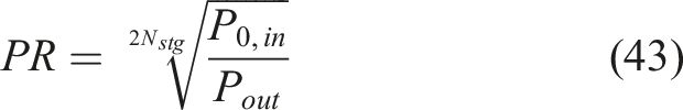

$\mathit{PR}=\sqrt[2N_{stg}]{\frac{P_{0,in}}{P_{out}}}$

(43)

Where the N _stg is the number of stage. When the method fails to make the program converge, the outlet pressure obtained from the last iteration is directly adopted.

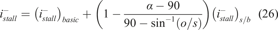
The next step is the calculation of choking. Choking is a special and important operating condition in axial flow turbine performance analysis. The accuracy of its prediction directly affects the result of turbine performance analysis. It can be found that different from the compressor performance prediction, the design operating point of the turbine may also be in the choke condition due to its high efficiency. As a general rule, the Mach number of unity at the throat is the judge criterion that the turbine enters the initial choke state. ¹ At this time, the supersonic zone runs through the entire cascade passage near the throat. But the throat area and loss model before the throat are absent. The entropy that is generated before the throat can only be determined on the basis of experience at the stage of preliminary design. Thus, the calculation may be biased. Therefore, another method is adopted. The outlet Mach number for the initial choking state on the order of 0.94 ± 0.03 is used as a judge criterion. ³

At the condition where the turbine is choked, the calculation method with given mass flow is difficult to converge or give reasonable results. The probable reason is that the mass flow does not increase with a further decrease in the downstream pressure when upstream pressure is fixed. Thus, adding a new routine for the calculation in the choke section is extremely necessary. The routine is modified on the basis of the calculation of the program in the non-choked section. The modifications are as follows: first is the input data. The assigned inlet mass flow rate is removed and replaced with the choking mass flow and assigned total-to-total pressure ratio, which is started from the critical pressure ratio. These two values can be directly substituted in the calculation rather than adjusting the outlet pressure to match the flow. Once the limit load conditions are reached, the routine will automatically stop. The deviation angle of the choked blade row is calculated by using the equation of continuity when the Mach number is larger than one. The detailed calculation diagram is shown in Figure 8. For the initial value of the choking condition, the equal stage pressure distribution based on the given total pressure ratio is taken because the given total pressure ratio can only be reflected in this respect in addition to the limit on the outlet pressure of the final stage. Otherwise, only the final stage pressure ratio changes when the given total pressure ratio of turbine increases in the calculation of turbine characteristic curve.

Figure 8.

Diagram of choke routine.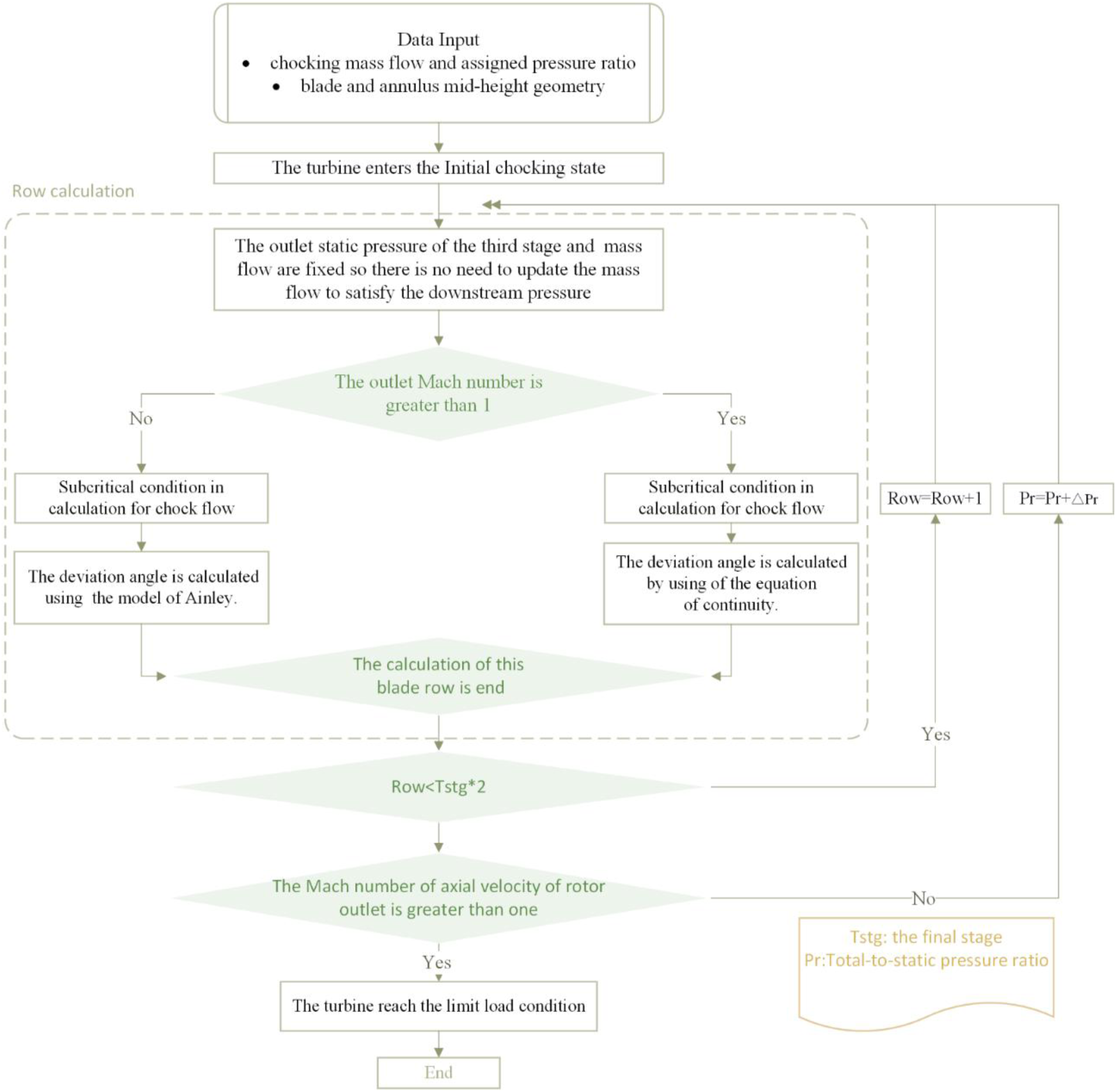

The run time for a single speed line with 20 mass flow points is typically less than 5 min on a PC with core i5 processor. In view of the blockage factor or work done factor, for multistage compressors, the blockage factor is the reflection of the phenomenon that the boundary layer of annular wall blocks air flow through the passage and then directly leads to the decrease in capability in generating the actual mechanical work. For multistage turbines, reheating is the focus of attention when considering the effect of the interstage interaction. In addition, the positive pressure gradient of the turbine cascade brings about the thinner boundary layer compared with the reverse pressure gradient of the compressor. Thus, the blockage factor is ignored.

Code validation cases

Two transonic axial turbines are selected to produce turbine performance maps that describe the flow and efficiency characteristics as a function of the rotational speed and pressure ratio. The overall design specifications of the five-stage LPT and GE PG9351FA turbine are given in Table 2. The ambient temperature and pressure are set to 15°C and 101.32 kPa, respectively.

Table 2.

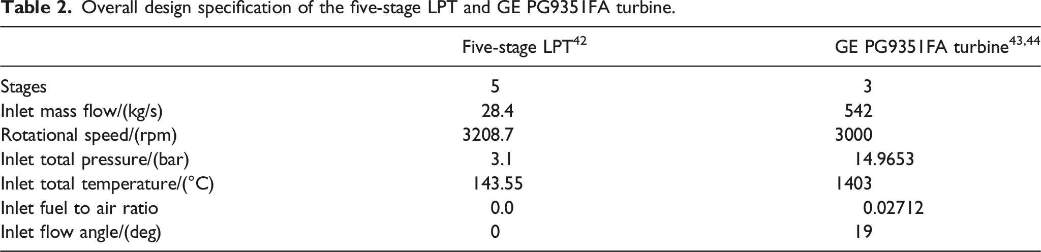
Overall design specification of the five-stage LPT and GE PG9351FA turbine.

	Five-stage LPT 42	GE PG9351FA turbine43,44
Stages	5	3
Inlet mass flow/(kg/s)	28.4	542
Rotational speed/(rpm)	3208.7	3000
Inlet total pressure/(bar)	3.1	14.9653
Inlet total temperature/(°C)	143.55	1403
Inlet fuel to air ratio	0.0	0.02712
Inlet flow angle/(deg)	0	19

The rotational speed and inlet total flow properties remain unchanged with the variations to the outlet static pressure used to move along the speed line to calculate each speed line on the map.

Five-stage LPT

The first set of results provided in this paper focuses on the performance characteristics of a scaled test turbine. The turbine is a part of the NASA/GE E³ component development and integration program. It is a five-stage, highly-loaded ( $\mathrm{\Delta }$ h/U ² =2.584), low through flow design featuring high outer wall slope using a 0.67 scaled E³ ICLS LP turbine. The scaled air turbine tests are arranged to determine the possible performance of the turbine in future ICLS engine tests. The design parameters mentioned below all come from the scaled air turbine tests. Cooling requirements have been minimized in tests, and only the nozzle of the first stage uses controlled purge air from the fifth-stage compressor bleed for seal blockage and disk rim purge. ⁴² For five-stage LPT, the unit is chosen for two reasons, the first is that the detailed geometry data and overall performance are available in NASA Technical report. ⁴² This is very helpful for program validation, especially if the program is built from scratch. The second reason is that turbine cases with large cooling air and detailed known cooling information distribution are very rare. The only case can be found is the GE PG9351FA turbine.

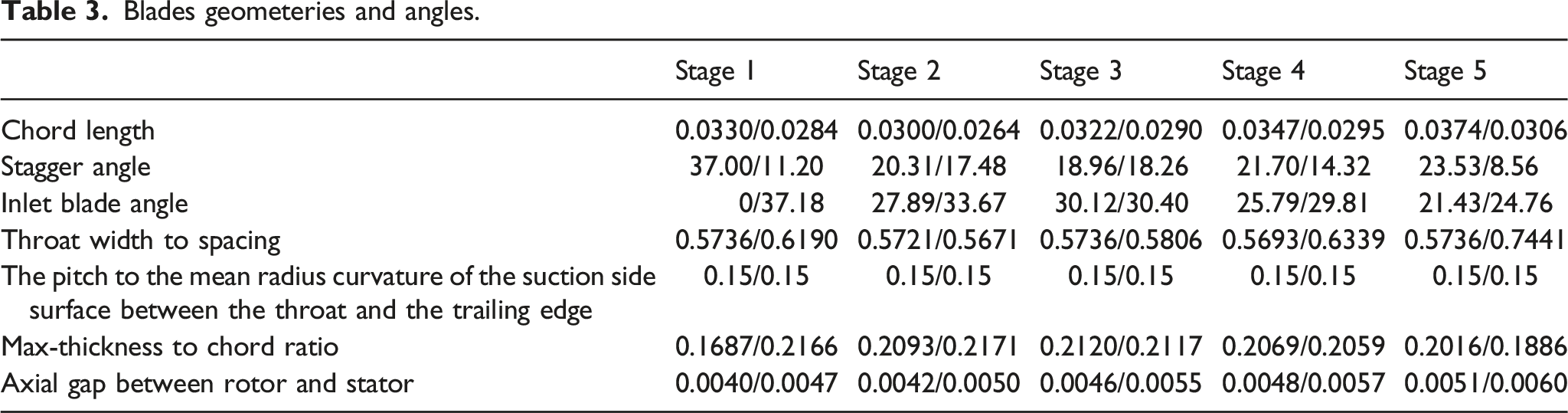
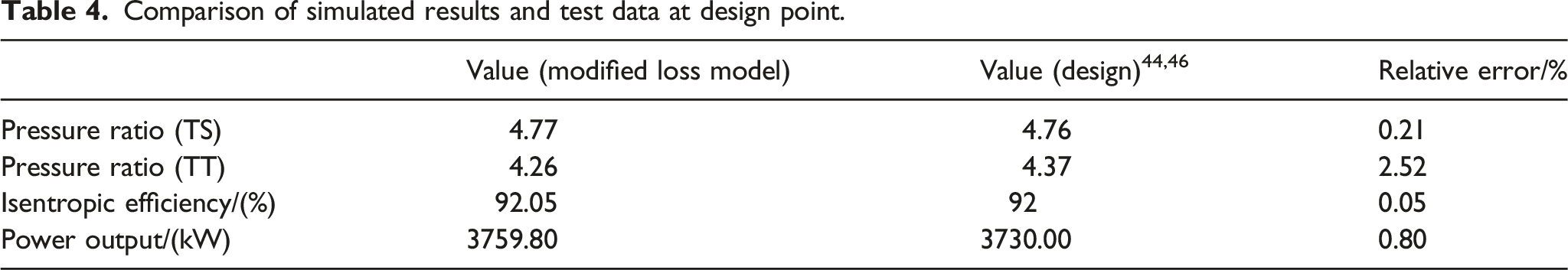
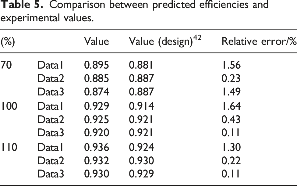
The thermodynamic performance of five-stage LPT under design condition is studied before the off-design calculation model of turbine is established. Figure 9 shows the comparison diagram of the calculated and final design meridional channels. The design point performance is verified as shown in Table 4. The detailed blade geometries and angles are shown in Table 3. In the calculation, the loss model of Craig and Cox is tuned by adding an empirical manual increment on the basis of the design point performance to obtain a better matching with the test data, as commonly mentioned in some literature. 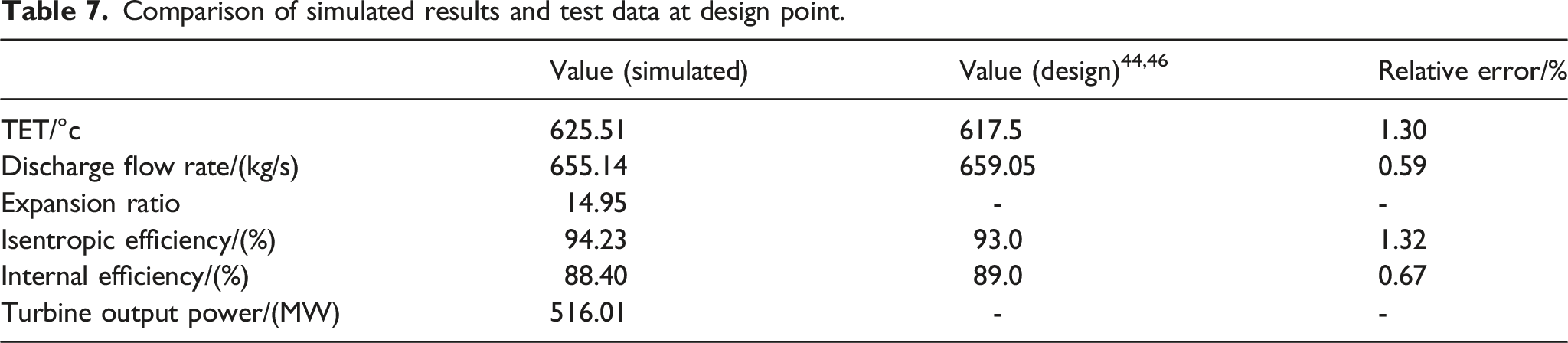⁴⁵ It can be seen from Table 4 that only the pressure ratio is slightly lower, the maximum difference is +2.52%, the other calculated parameters are consistent with the data provided by the manufacturer. It is rational to say that a slight error from the experimental data is normal. For cases where the cascade and profile characteristics are unknown, the 1D prediction is only a rough estimation.

Figure 9.

Comparison diagram of calculated and final design meridional channel.

Table 3.

Blades geometeries and angles.

	Stage 1	Stage 2	Stage 3	Stage 4	Stage 5
Chord length	0.0330/0.0284	0.0300/0.0264	0.0322/0.0290	0.0347/0.0295	0.0374/0.0306
Stagger angle	37.00/11.20	20.31/17.48	18.96/18.26	21.70/14.32	23.53/8.56
Inlet blade angle	0/37.18	27.89/33.67	30.12/30.40	25.79/29.81	21.43/24.76
Throat width to spacing	0.5736/0.6190	0.5721/0.5671	0.5736/0.5806	0.5693/0.6339	0.5736/0.7441
The pitch to the mean radius curvature of the suction side surface between the throat and the trailing edge	0.15/0.15	0.15/0.15	0.15/0.15	0.15/0.15	0.15/0.15
Max-thickness to chord ratio	0.1687/0.2166	0.2093/0.2171	0.2120/0.2117	0.2069/0.2059	0.2016/0.1886
Axial gap between rotor and stator	0.0040/0.0047	0.0042/0.0050	0.0046/0.0055	0.0048/0.0057	0.0051/0.0060

Table 4.

Comparison of simulated results and test data at design point.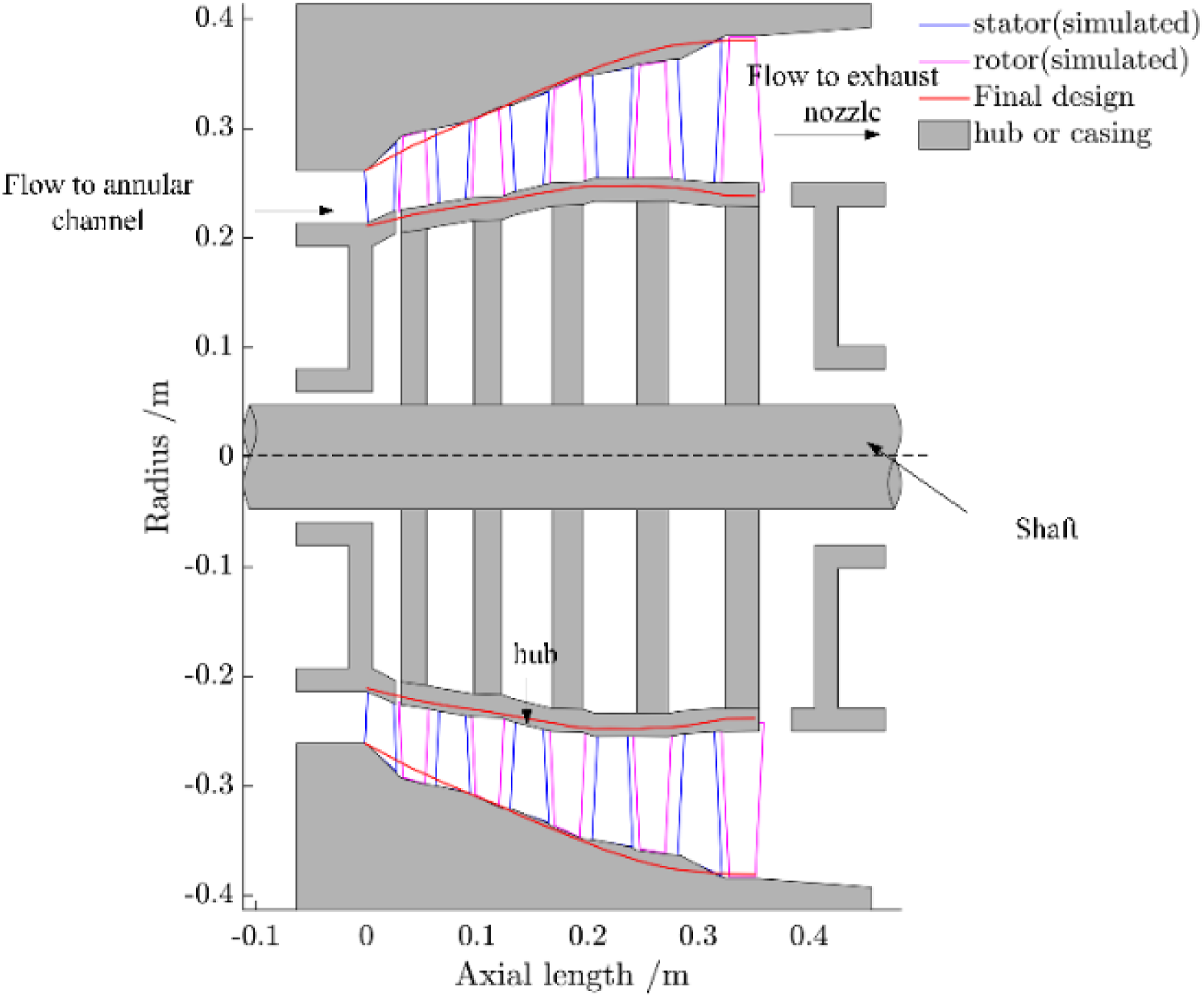

	Value (modified loss model)	Value (design)44,46	Relative error/%
Pressure ratio (TS)	4.77	4.76	0.21
Pressure ratio (TT)	4.26	4.37	2.52
Isentropic efficiency/(%)	92.05	92	0.05
Power output/(kW)	3759.80	3730.00	0.80

Figures 10 and 11 shows the mass flow and efficiency comparisons between the experimental and calculated characteristics under variable operating conditions (70%, 100% and 110%Nd respectively). The calculated mass flow values have good conformity in terms of magnitude and trends with the experimental values but the predicted efficiencies at low pressure ratio are a slightly pessimistic. A detailed comparison between predicted efficiencies and experimental data at these three rotational speeds is shown in Table 5. The relative error is between 0.11% and 1.64%, within the reasonable range.

Figure 10.

Massflow rate component of five-stage LPT characteristic.

Figure 11.

Total-to-total isentropic efficiency component of five-stage LPT characteristic.

Table 5.

Comparison between predicted efficiencies and experimental values.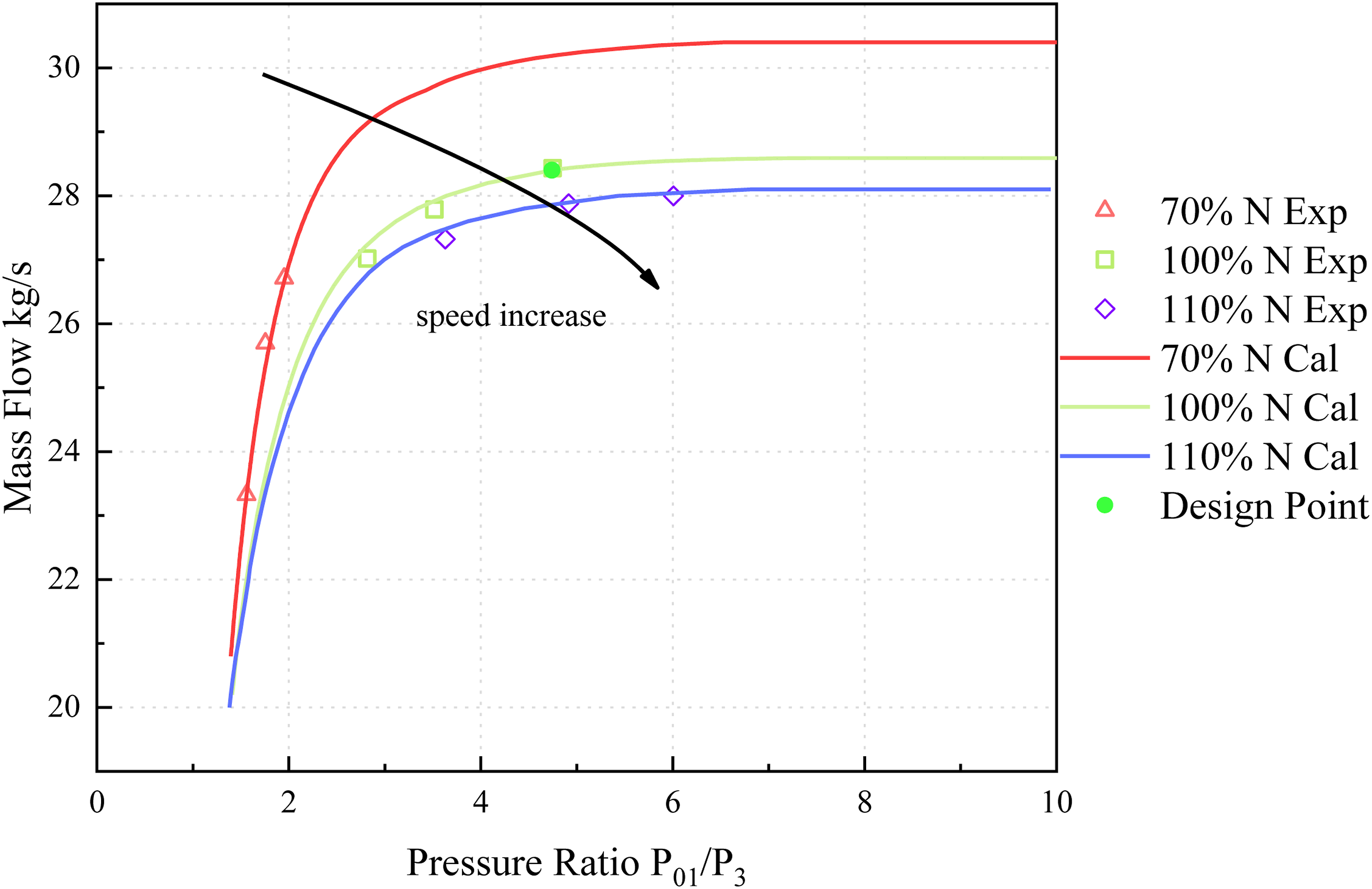

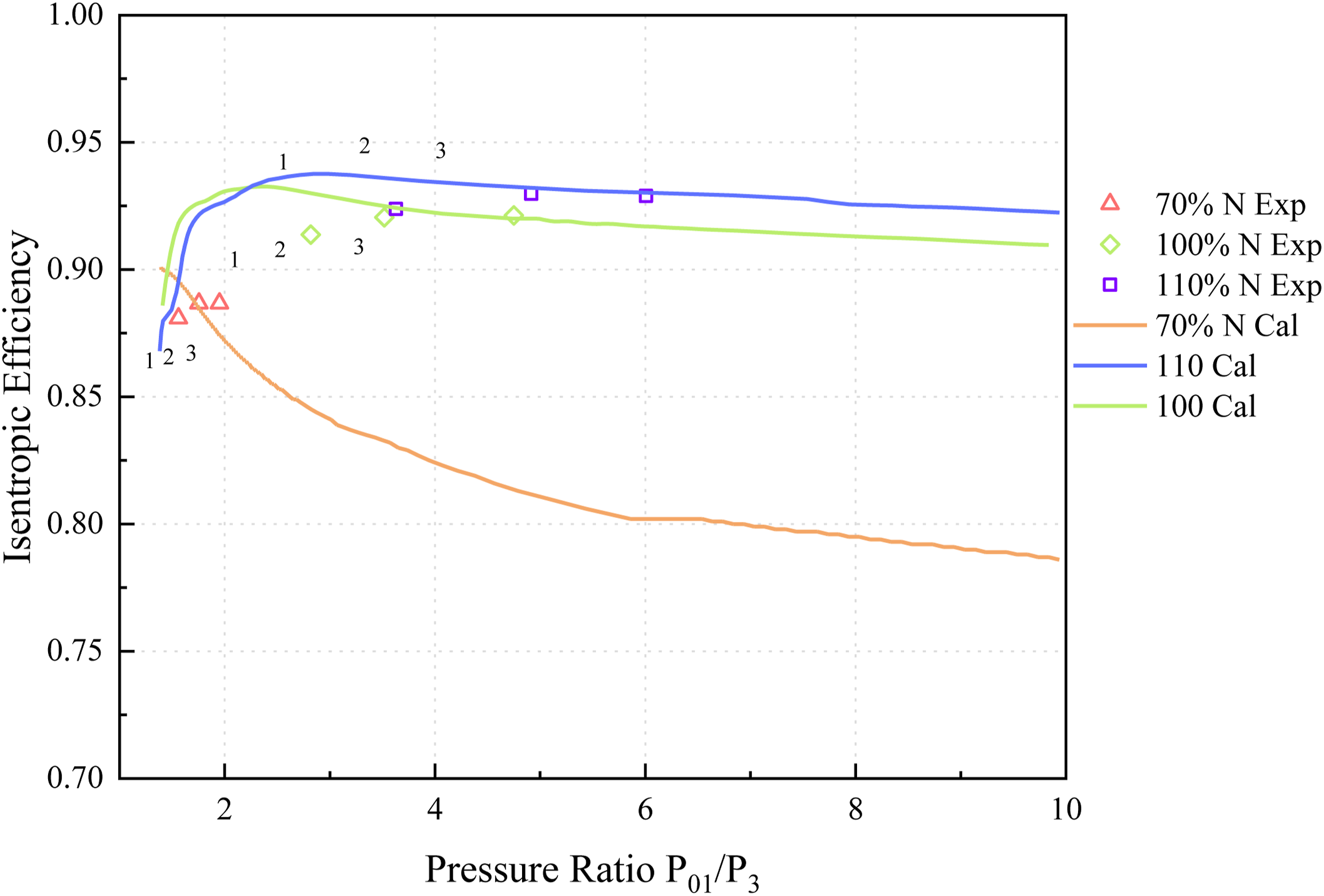
(%)		Value	Value (design) 42	Relative error/%
70	Data1	0.895	0.881	1.56
	Data2	0.885	0.887	0.23
	Data3	0.874	0.887	1.49
100	Data1	0.929	0.914	1.64
	Data2	0.925	0.921	0.43
	Data3	0.920	0.921	0.11
110	Data1	0.936	0.924	1.30
	Data2	0.932	0.930	0.22
	Data3	0.930	0.929	0.11

There are two points on the characteristic curve need to be determined. First is the initial choke point. The second is the critical pressure ratio point. If the back pressure decreases, the airflow can only expand unlimitedly outside the cascade, and the pressure of the blade surface is no longer affected by the further decline in back pressure. Then the tangential velocity, which determines the turbine output work, dose not increase, and the limit load of the cascade is determined. For the five-stage LPT with a relatively low inlet temperature and pressure, this criterion should be followed. However, for GE PG9351FA turbine, the load of every blade is very high. Therefore, this paper conservatively estimated the limit load state (axial outlet velocity is 0.6). It can be seen from the figure that the critical pressure ratio drops with the decrease in rotational speed decreases, and the mass flow rate at the initial choking point increases with the decrease in reduced rotational speed.

Cooled turbine

After sufficient reliability is achieved with the five-stage LPT, it is time to move on to the predict the performance of the GE PG9351FA turbine with the feature of such a high cooling air flow and transonic working condition. Because the cooling and mixing losses need to be considered, the calculation becomes more complicated and more difficult to converge than the five-stage LPT. Therefore, the choice of the initial value is especially important at this time.

Because of business secrecy, the geometry information of GE PG9351FA turbine cannot be obtained in the open literature, let alone the performance under part load conditions even though the GE PG9351FA turbine was developed at least 10 years ago. Fortunately, part of the calculated characteristic curve of GE PG9351FA turbine is given in literature, ⁴³ which can be used as a reference. However, the curve is calculated by Flügel formula and internal flow and cooling loss are not considered in detail. Morever, the literature does not give the definition of internal efficiency. So the data in the literature cannot be used as an absolute reference value. The trend and shape of the curve can be considered.

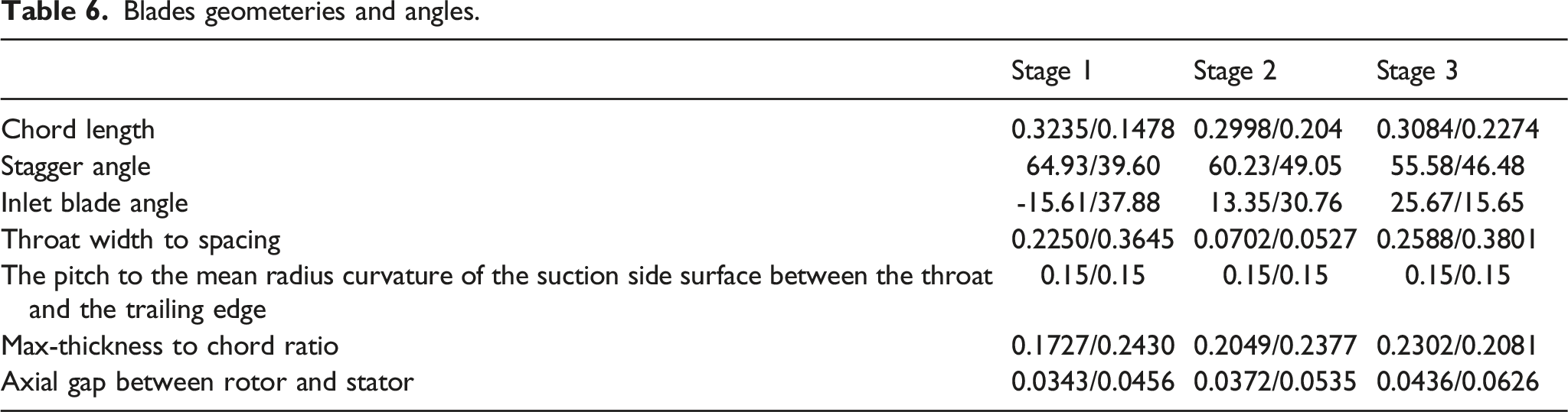
The GE PG9351FA turbine is designed in three stages with the rotational speed of 3000 r/min. Constant meridional diameter is adopted, and the stage power output is relatively large compared with the five-stage LPT. The detailed geometry and thermodynamic performance at design point have been studied in detail. The GE PG9351FA turbine annulus is shown in Figure 12. Stator contours are shown in blue and rotor contours are shown in red. The detailed blade geometries and angles are shown in Table 6.

Figure 12.

GE PG9351FA turbine annulus.

Table 6.

Blades geometeries and angles.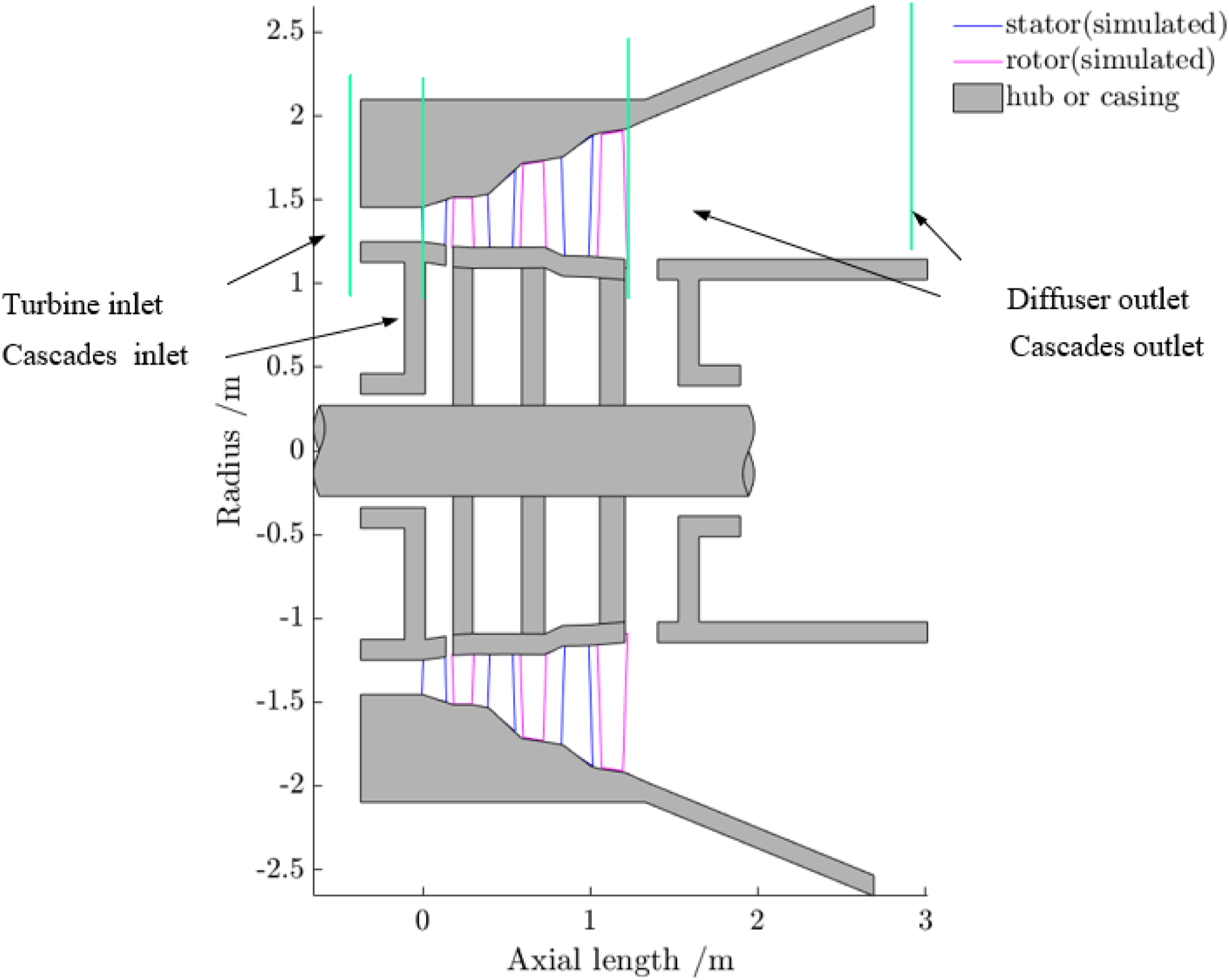

	Stage 1	Stage 2	Stage 3
Chord length	0.3235/0.1478	0.2998/0.204	0.3084/0.2274
Stagger angle	64.93/39.60	60.23/49.05	55.58/46.48
Inlet blade angle	-15.61/37.88	13.35/30.76	25.67/15.65
Throat width to spacing	0.2250/0.3645	0.0702/0.0527	0.2588/0.3801
The pitch to the mean radius curvature of the suction side surface between the throat and the trailing edge	0.15/0.15	0.15/0.15	0.15/0.15
Max-thickness to chord ratio	0.1727/0.2430	0.2049/0.2377	0.2302/0.2081
Axial gap between rotor and stator	0.0343/0.0456	0.0372/0.0535	0.0436/0.0626

In this way, at least the accuracy of the turbine performance analysis at design condition can be guaranteed.

Table 7 shows the performance results and reference data. The TET, discharge flow rate, isentropic efficiency, and output power are considered. The TET is 1.3% higher than the final design value. The discharge flow rate is 0.59% higher than the final design value. The isentropic efficiency is 0.15% higher than the final design value. The internal efficiency is 0.67% lower than the final design value. Overall, the furthest discrepancy of 1.3% meets the requirements of calculation accuracy. The predicted performance results show good correspondence with the turbine design.

Table 7.

Comparison of simulated results and test data at design point.

	Value (simulated)	Value (design)44,46	Relative error/%
TET/°c	625.51	617.5	1.30
Discharge flow rate/(kg/s)	655.14	659.05	0.59
Expansion ratio	14.95	-	-
Isentropic efficiency/(%)	94.23	93.0	1.32
Internal efficiency/(%)	88.40	89.0	0.67
Turbine output power/(MW)	516.01	-	-

Figures 13 and 14 show the performance of GE PG9351FA turbine under variable working conditions (70%, 75%, 80%, 90% and 100% Nd). In fact, for the performance analysis of the turbine, the further the speed deviates from the design speed, the more difficult it is to predict more accurately. This depends on the convergence and stability of the program.

Figure 13.

Internal efficiency component of GE PG9351FA turbine characteristic.

Figure 14.

Massflow rate component of ge pg9351fa turbine characteristic.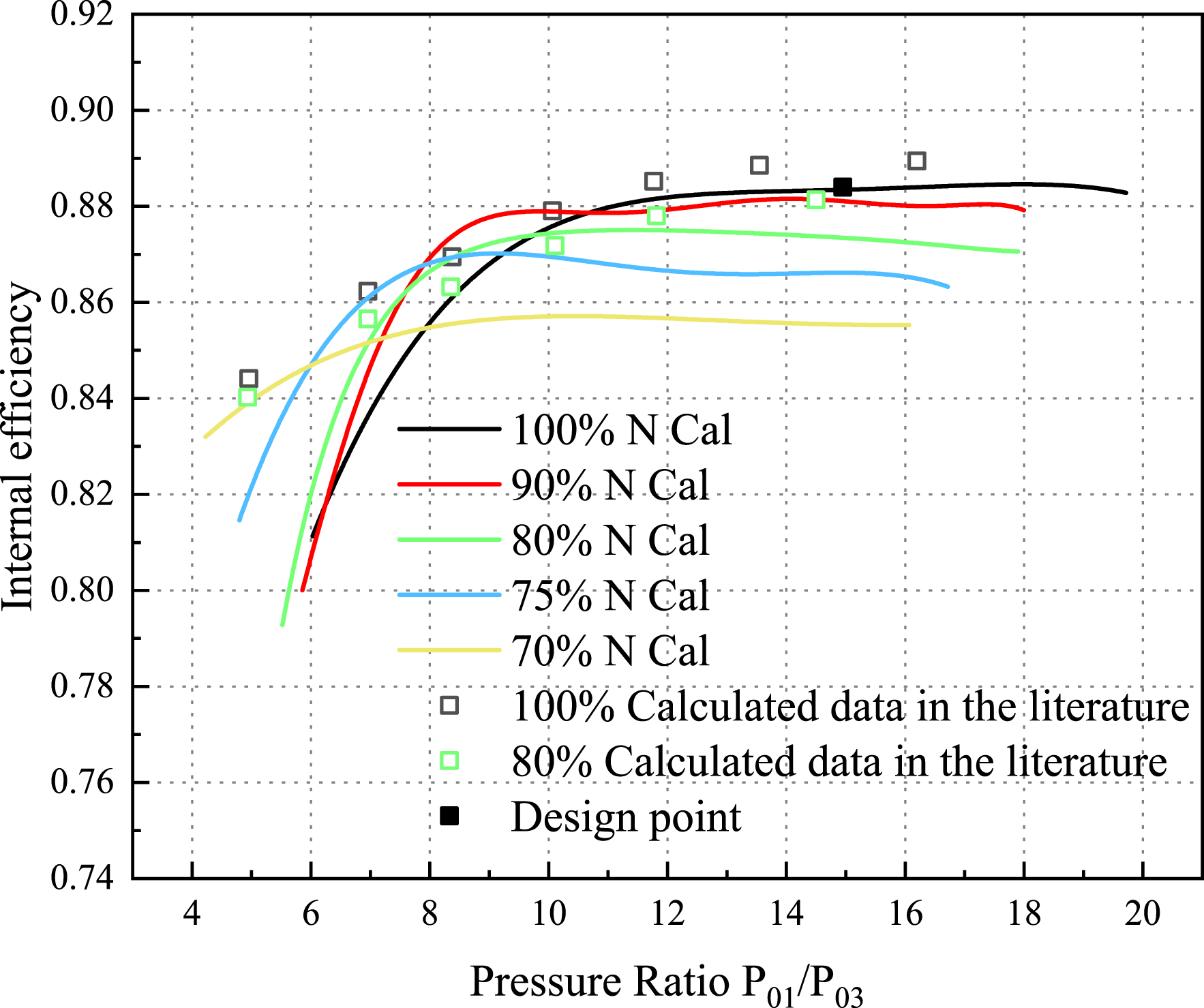

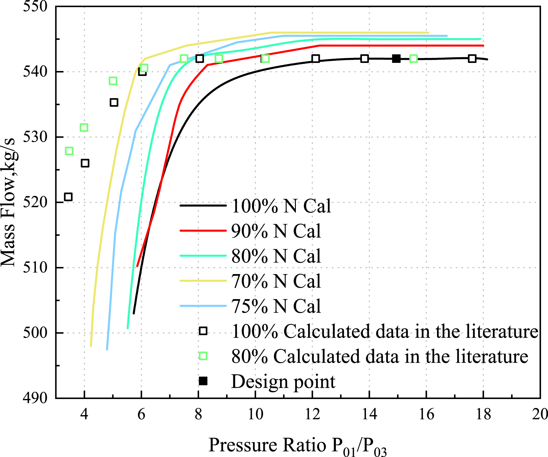
It can be seen from Figure 14 that in each rotational speed, the mass flow rises with the increase in the total-to-total pressure ratio until its maximum value is reached. The calculated data are consistent with the general trend of the data in open literature. But in non-choking condition, there is a certain deviation between the calculated values in the literature and those in this paper. The possible reason is that internal flow and cooling loss are not considered in detail when using Flügel equation. The same is true of the efficiency characteristic curve. In Figure 13, the internal efficiency shows an increasing trend with the increase of rotational speed, and its operating range becomes larger. At high speed and pressure ratio, the internal efficiency is almost constant because the forward pressure gradient allows the blade to operate over a wide incidence angle without adding too much loss. When the turbine is operating at the design speed, the internal efficiency reaches its maximum value at the design point. Since the five-stage LPT is subsonic, it is rational that its highest efficiency locates at non-choking condition which deviates from the design point. In terms of the variation trend of gas turbine performance with pressure ratio and rotational speed, the calculated characteristic curve is reasonable, which explains the rationality of the calculated results to a certain extent.

Conclusion

The proposed analysis program forms a complete and detailed prediction for air-cooled turbine performance, which has built-in capability for cooling and diffuser. In addition, a choke routine, which can realize the calculation of choked flow up to limit load conditions, is performed so that the problem that the program fails to converge near or at the initial choked condition can be solved. To evaluate this 1D program, five-stage LPT and GE PG9351FA turbine is detailed simulated at design and off-design conditions. For five-stage LPT, the validation result shows that although the total-to-total pressure ratio is slightly conservative, this method achieves the required forecast precision. For GE PG9351FA turbine, from the variation trend of turbine performance with pressure ratio and rotational speed, it can be seen that this program has the capability of predicting the performance reasonably to some extent. In the future, more parameters are known and the models can be further proved.

The obtained turbine maps can be applied or this 1D mid-span program directly coupled into the whole air-cooled modern GT performance simulation and further simultaneous optimization of the cycle and component aerodynamic parameters at the system level, which is of great value.