Sage Journals: Discover world-class research

Abstract

A novel optimisation process has been proposed in this paper to maximize the aerodynamic efficiency of a modern fan blade while satisfying the structural constraint imposed by the material limits. The method developed is based on the discrete adjoint for the aerodynamic efficiency sensitivity evaluation with the structural constraint provided by a response surface method for the structural stress. To facilitate a large number of sampling points required in the response surface generation, a fast, meshless method was used for the stress calculations. The method was applied to the optimisation of a practical fan blade, representative of modern, high-bypass-ratio turbofan jet engines. It is demonstrated that the fan blade efficiency can be improved by 0.6% while maintaining the stress below a prescribed value of 500 MPa assuming a titanium alloy material. It is shown that without the stress constraint, the efficiency benefit is larger, namely 0.9% but the maximum stress value increases considerably beyond the material’s acceptable criterion, to almost 1000 MPa. The method is built in a modular way and can be adapted to accommodate a range of different turbomachinery blade designs. Flutter analysis for the optimised fan blade has also been carried out due to its practical importance.

Keywords

Adjoint multidisciplinary optimisation transonic axial fan blade aerodynamic efficiency maximum stress

Introduction

Turbomachinery is a complex engineering system with complicated flow phenomena and interactions between various disciplines, that takes a very long time to design and is reliant on the experience of the designers. New turbomachinery designs need to strive for high aerodynamic efficiency, low noise and low environmental impact while ensuring safety and reliability. In today’s competitive market, a company’s ability to develop successful products, such as turbomachinery blades, also relies on shorter time scales and lower overall costs. The rapid development of computational capabilities has led to a large number of computational design optimisation methods being developed for turbomachinery.¹ In the field of fan blade optimisation, the most used test cases are the NASA cases, for which extensive tests had been done: Rotor 67² and NASA SDT Fan.³ The two cases offer good benchmarks for developing methods and predicting the aerodynamic performances^4–6 or noise levels.^7–9 However, the majority of the blade optimisation work for high-bypass-ratio aero-engine fan designs refers to mono discipline studies, mostly for improving aerodynamic performance. A good example of a fan blade monodisciplinary optimisation is the genetic algorithm optimisation of rotor 67 based on 56 blade design parameters, having a single objective function (entropy) and two aerodynamic constraints (mass flow rate, pressure ratio) developed by Oyama et al.¹⁰ Due to the prohibitive costs of the high-fidelity CFD models coupled with genetic algorithms, their research focused more on developing response surface models. Such an application for aerodynamic optimisation of fan blades was also reported in,¹¹ in which the optimisation of rotor 67 was conducted for a linear combination of efficiency and pressure ratio based on a polynomial response surface model coupled with a genetic algorithm.

Lian and Liu¹² included the blade weight along with the aerodynamic performance as objective function and coupled a GA with second-order polynomial response surface metamodels in one of the early multidisciplinary optimisations of a transonic fan blade. A year later, the same authors have added a response surface for the maximum von Mises stress that was used as a constraint.¹³ However, the structural analysis did not account for the change in blade pressure distribution or for the presence of the blade root. It was also fully reliant on low fidelity surrogate models for both aerodynamic and structural computations.

Extensions of this work were performed by Pierret et al.¹⁴ and addressed a multipoint optimisation based on three operating points, but without considering the aerodynamic load in the structural analysis. With the development of new optimisation algorithms, similar studies started moving away from coupling genetic algorithms with response surfaces, towards adjoint based optimisations. The main motivation is that the computation for the gradients by the adjoint method, in a gradient based optimisation method, is independent of the number of design variables and requires only a relatively small number of additional computations equal to the number of objective functions.¹⁵ This allows for much faster gradient computations for design optimisation that require a large number of design variables, such as detailed turbomachinery blade designs. Carini et al.¹⁶ developed an integrated aero-structural coupled adjoint optimisation process which they applied to aircraft wing design.

In turbomachinery applications, Verstraete et al.¹⁷ have used both aerodynamic and structural disciplines in a decoupled adjoint optimisation process to increase the efficiency of automotive radial turbines while constraining the maximum stress to a predefined limit. They have further developed this work into a multipoint approach, that considers three operating points in the aerodynamic computations.¹⁸ Other studies, e.g., that performed by Trompoukis et al.¹⁹ couple aerodynamics with aerothermal performances for axial turbines. The majority of fan blade optimisations based on adjoint methods are also purely aerodynamic. Luo et al.²⁰ achieved the reduction in the entropy production per unit of mass flow rate combined with the constraints of mass flow rate and total pressure ratio in a multipoint optimisation approach based on a continuous adjoint approach for the gradients. Some recent fan tests have been conducted with a series of adjoint based optimisation studies on the industrial modern turbofan geometry, designed by Rolls-Royce, referred to as Vital fan blade.^21–23 Due to the importance on noise emissions and the noise production mechanisms of high-bypass-ratio gas turbine fans, Long et al.²⁴ focused on a coupled aerodynamic and acoustic adjoint based multidisciplinary design optimisation (MDO) approach, targeting an improvement of the aerodynamic efficiency while lowering noise levels. Their study on the Vital fan blade showed that these requirements can be met simultaneously. For the high-bypass-ratio fan blades optimisation, an aero-structural optimisation based on the adjoint method is proposed in this paper. From the few existing papers using other optimisation algorithms that couple the aerodynamic computations with the structural analysis, only the work of one group considers the blade root,²⁵ without, however, including the gas loads in the structural analysis. The main goal of this work is to develop a novel optimisation process able to maximize the aerodynamic efficiency of a fan blade while respecting the structural constraints as imposed by the material limits with sufficient accuracy for the initial design phase but significantly reducing the time scale and therefore overall design cost. In this context, the novelty of the method presented here refers to the coupling of an adjoint-based aerodynamic optimisation process with a response surface based model for constraining the maximum stress on the fan blade. A prototype of an MDO based on an automated integrated CAD-CFD-FEA system is developed for a transonic fan blade. The methodology is modular, which allows different models to be used, with different level of complexity and fidelity, allowing the user to define their own, customized process, based on their requirements. The structure of the process allows for flexibility in balancing the desired accuracy versus computational time.

Methodology

The following section describes the methods and tools used in the fan multidisciplinary optimisation process.

Test case

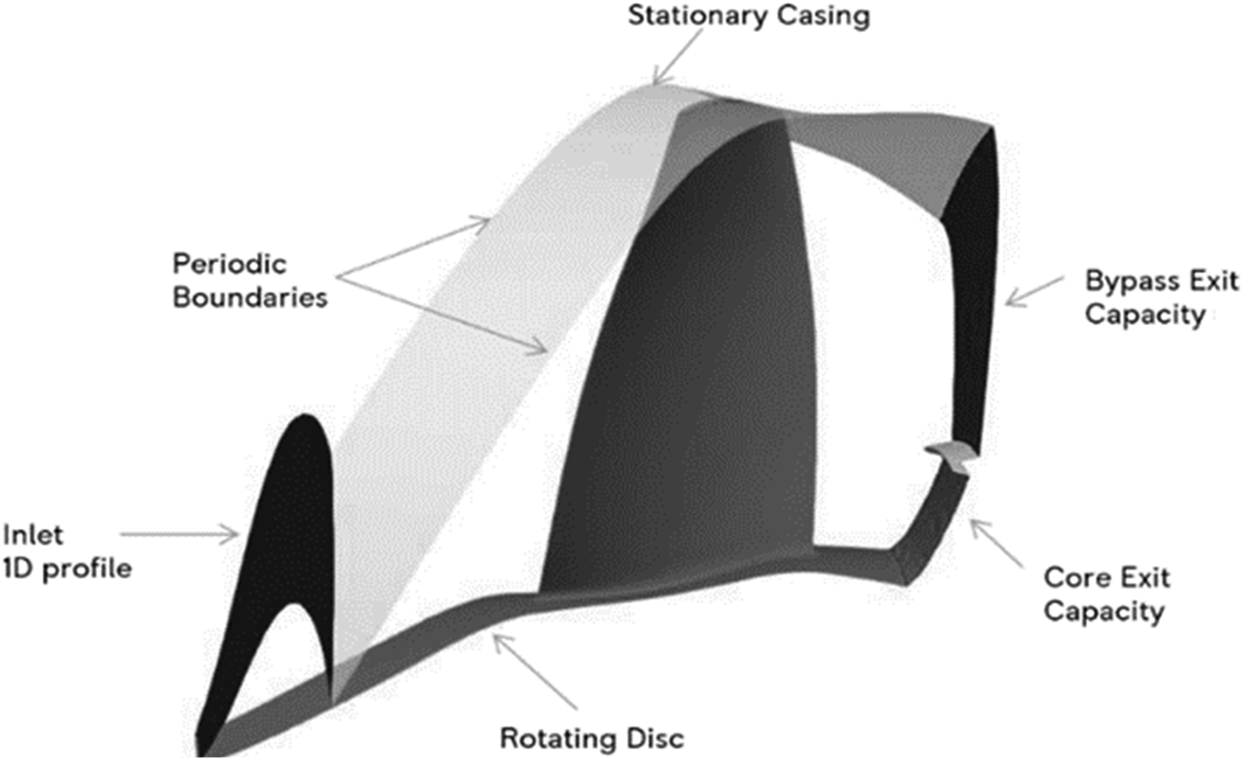
The case selected for being representative of a modern fan is the Rolls-Royce VITAL fan.^21–23 The VITAL blade geometry considered was the test rig scale solid fan blade geometry. Figure 1 shows the fan blade geometry, as well as the boundary conditions used for the CFD simulation.

Figure 1.

The VITAL fan blade geometry and CFD domain.²³

CFD Setup

All the simulations presented here are RANS computations using the Rolls-Royce in-house code, HYDRA²⁶ with the Spalart-Allmaras (SA) turbulence model. While there are a number of choices for the RANS solver, the corresponding Adjoint solver is only available for the SA one equation model. The inlet boundary conditions are specified as radial distribution of total pressure, total temperature, and inlet flow angles, while at the outlet, a value for circumferentially mixed-out and radially mass-averaged capacity is imposed. The walls are considered adiabatic viscous no-slip walls. The rotational speed was set to 809.136 rad/s. The validation of the CFD simulation results using the same approach for the spanwise profiles of the fan aerodynamic performance compared against experimental data is presented in.²⁴

For all optimisation studies presented here, Rolls-Royce Hydra Adjoint is used to provide the gradients of the aerodynamic quantities of interest with respect to the design parameters based on a discrete adjoint approach.²⁷ The primal solver is coupled with the discrete adjoint solver, and they share the discretization method, solver procedure and solver settings. The multi-block structured meshes were automatically generated using the in-house software PADRAM.²⁸ An H-O-H mesh topology is used in the blade-to-blade section.

Uniform grids are applied both axially and circumferentially to the rotor upstream H block. Based on a mesh dependence study for this setup conducted in,²⁴ mesh-independent predictions (less than 0.25% changes relative to the finest mesh predictions) of the aerodynamic parameters can be obtained by using 122 axial grids, 150 radial grids and 106 circumferential grids. The radial mesh is clustered towards the hub and casing to resolve the boundary layers on both sides. The O-mesh around the fan blade achieves y⁺ values of the order of one. For the blade tip gap region, a butterfly mesh topology and 40 layers are used to capture the tip leakage flow. The resulting mesh consists of 6.013 million points for a single-blade passage and can be visualised in Figure 2.

Figure 2.

Computational Mesh: (a) Blade; (b) Radial slice mid-span, zoomed near the leading edge.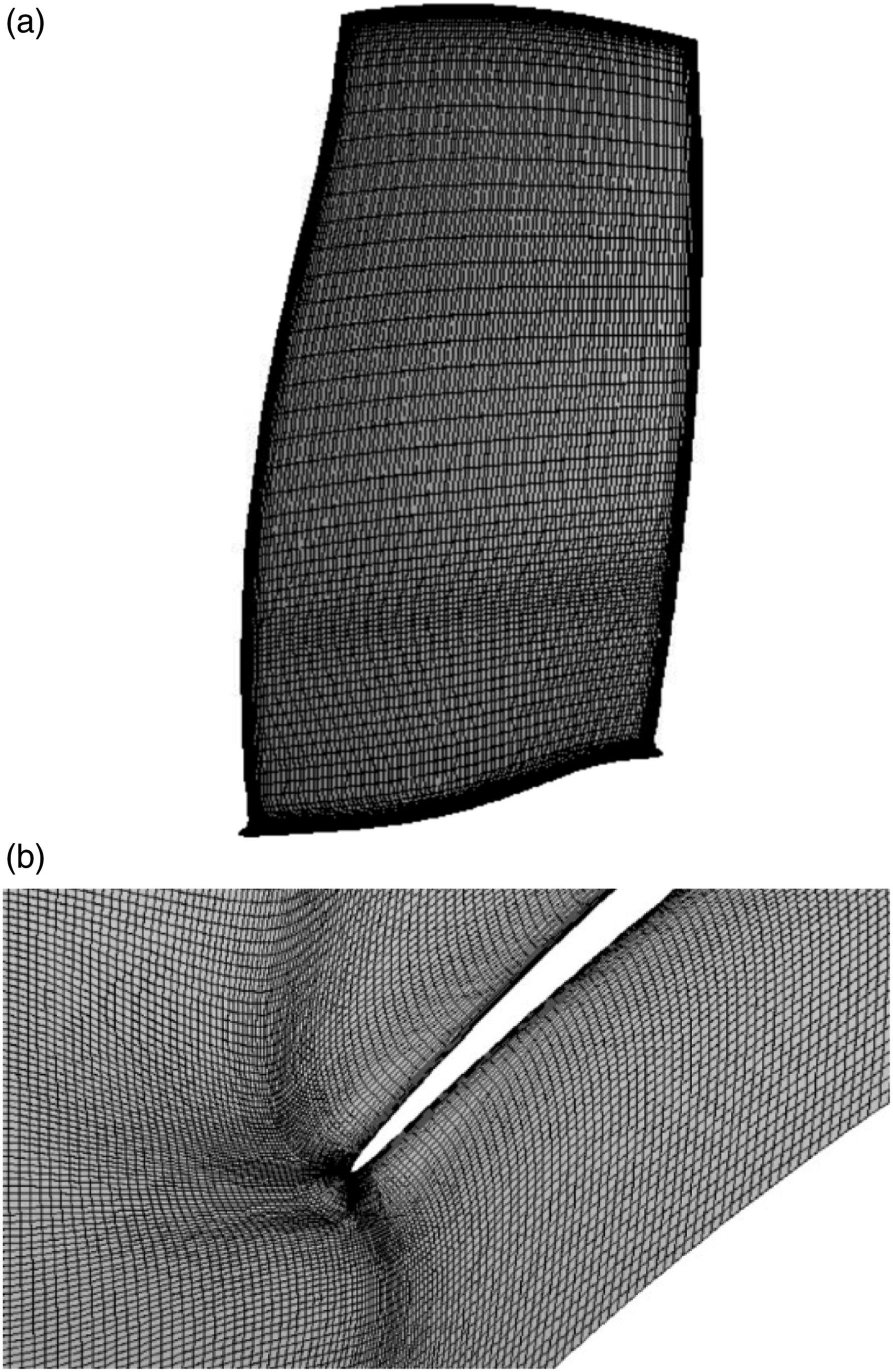

Geometry parametrisation

The definition of the geometry parametrization is a critical factor in producing or conducting a successful optimisation. For the optimisation of the VITAL fan blade, the aerofoil shape is not directly parametrized, but rather the geometry parametrization is defined through PADRAM’s Engineering Design Parameters (EDP), which comprise a set of intuitive geometry manipulation handles based on first principles. Each EDP controls a particular Degree of Freedom (DOF) for the geometry.

The seven DOFs controlling the aerofoil shape and used for the optimisation are: Sweep (axial movement of the section), Lean (circumferential movement of the section), Skew (rotation about the section’s centroid), Leading Edge (LE) and Trailing Edge (TE) recambering, along with two additional DOFs controlling the locality of the LE and TE recambering, such that low values of these parameters cause very localized camber line alterations, and vice-versa. Sufficiently large values can propagate the perturbations through the aerofoil, thus providing complete control over the camber line and curvature of the aerofoil, including the possibility of obtaining a negative camber. Sweep range was set to [−20, 20] mm, while for the other parameters the rage was [−3, 3] degree. The first five EDP are illustrated in Figure 3 for an aerofoil section.

Figure 3.

Design parameters employed for VITAL optimisation.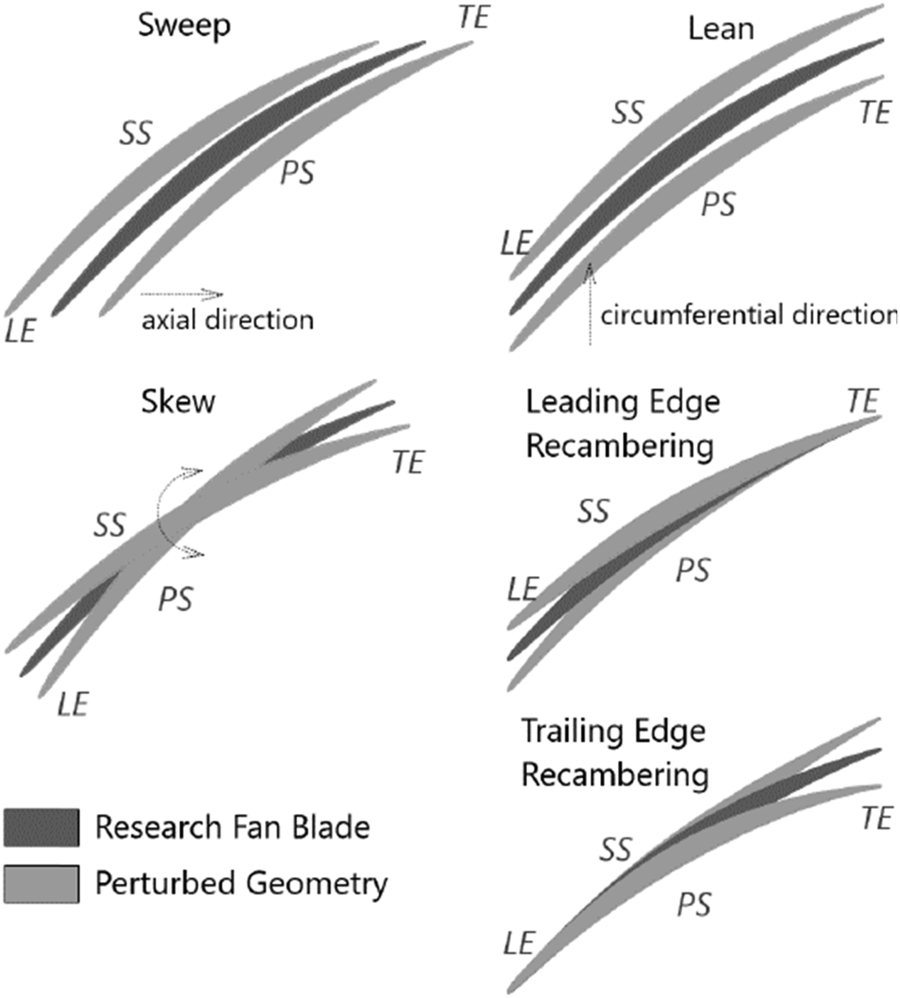

The EDPs are applied at five aerofoil control sections distributed through the blade span at 25%, 50%, 75%, 87.5% and 100%. The approach leads to a total of 35 design parameters, arranged in the design vector. The values of the deformations applied as a function of the blade span are achieved through smooth cubic B-spline interpolation, with multiple control points via the control sections. The geometry was fixed below 5% of span, to allow attaching the same blade root to all designs for structural evaluations.

Structural model

Adding the blade root to the aerodynamic blade shape

The stress analysis was done by attaching the blade root represented in dark grey in Figure 4 (left) to the aerodynamic blade shape, represented in lighter grey in the same figure. This was achieved by using SolidWorks CAD package. It is very important how the geometry creation and manipulation are handled. To avoid introducing stress concentration in the connection region, the blade root was created to ensure tangency to the aerodynamic blade shape in the contact region. Figure 4 (middle) shows stress concentrators in the contact region when tangency condition is not met, while Figure 4 (right) shows a smooth stress distribution when blade root tangency to the blade is ensured. To further ensure smooth transition for each of the newly created geometries during the optimisation process, the datum blade shape below 5% span is preserved for all generated geometries.

Figure 4.

Fan bade with root attached (left); Vital Datum – Stress distribution without (middle) and with blade root tangency (right).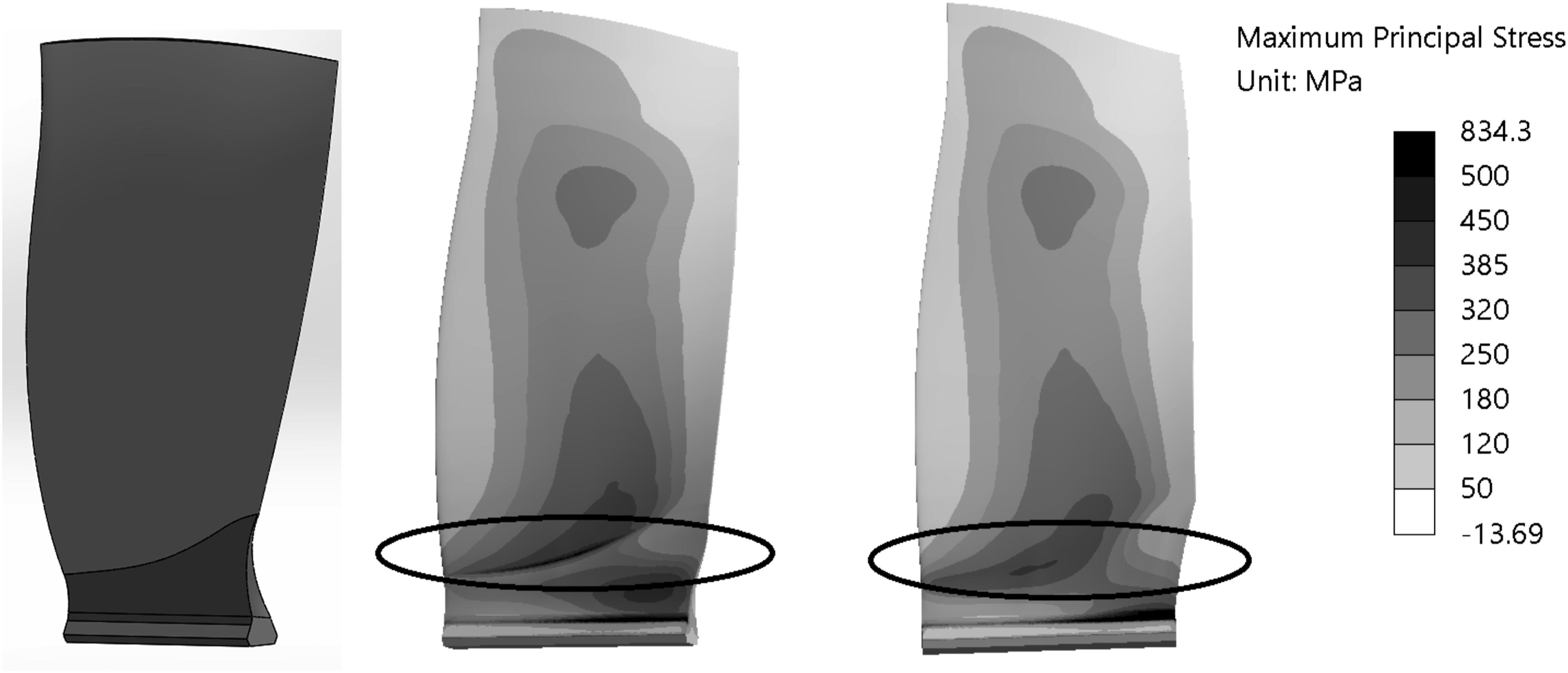

The blade root addition is very important for the correct reading of the value of the maximum stress on the blade. Two different structural analyses have been conducted and compared to show this. One analysis was done with the blade root added, while a second analysis did not include it. The case without the blade root had the hub section fixed. Without any fillet in the hub region, the sharp edge would introduce a singularity. To avoid this, an artificial fillet is introduced for this structural analysis. Although the stress distribution computed on the blades without the blade root (Figure 5 (left)) is similar to the stress distribution on the blade with the blade root (Figure 5 (right)), due to the simplification of not having the root and fixing the blade in the hub region, the maximum stress on the blade is in the region of this fillet and is with 32.5% larger than the maximum stress on the blade computed with the blade root attached.

Figure 5.

Vital Datum – Stress distribution without (left) and with blade root (right).

It is important that the CAD geometry manipulation for attaching the blade root to each of the aerodynamic blade geometry generated for the optimisation is done automatically, by means of a script written for SolidWorks. The aerodynamic blade geometry has its input in a neutral format (.stp) and combines the two solids into one solid that is also exported in.stp format. The automation of this process is crucial for integrating it directly in the computations that are executed during an optimisation process or in the generation of a response surface method. The rooted blade geometry is further used by the script that does the automatic stress computations.

Stress computation validation

To reduce the computational cost, a meshless method provided by the SimSolid software,²⁹ based on breakthrough extensions to the theory of external approximations³⁰ was selected for performing the stress analysis and building up the response surface. The SimSolid approach and the verification of the stress results by comparison with Ansys Mechanical are reported below.

For the static structural analysis, the surfaces coloured in lighter grey on the blade root (Figure 4 (left) were fixed. Both the centrifugal and the aerodynamic loads were applied.

First, the aerodynamic load was applied in Ansys Mechanical by mapping the pressure distribution from the CFD results obtained in Hydra. The contribution of the aerodynamic load is analysed for the datum geometry based on the results reported in Figure 6, where the stress distribution on the blade is reported for both cases, without (left) and with (right) aerodynamic load added.

Figure 6.

Stress distribution on the fan blade computed without (left) and with aerodynamic load (mapping of the pressure distribution in Ansys Mechanical) (right).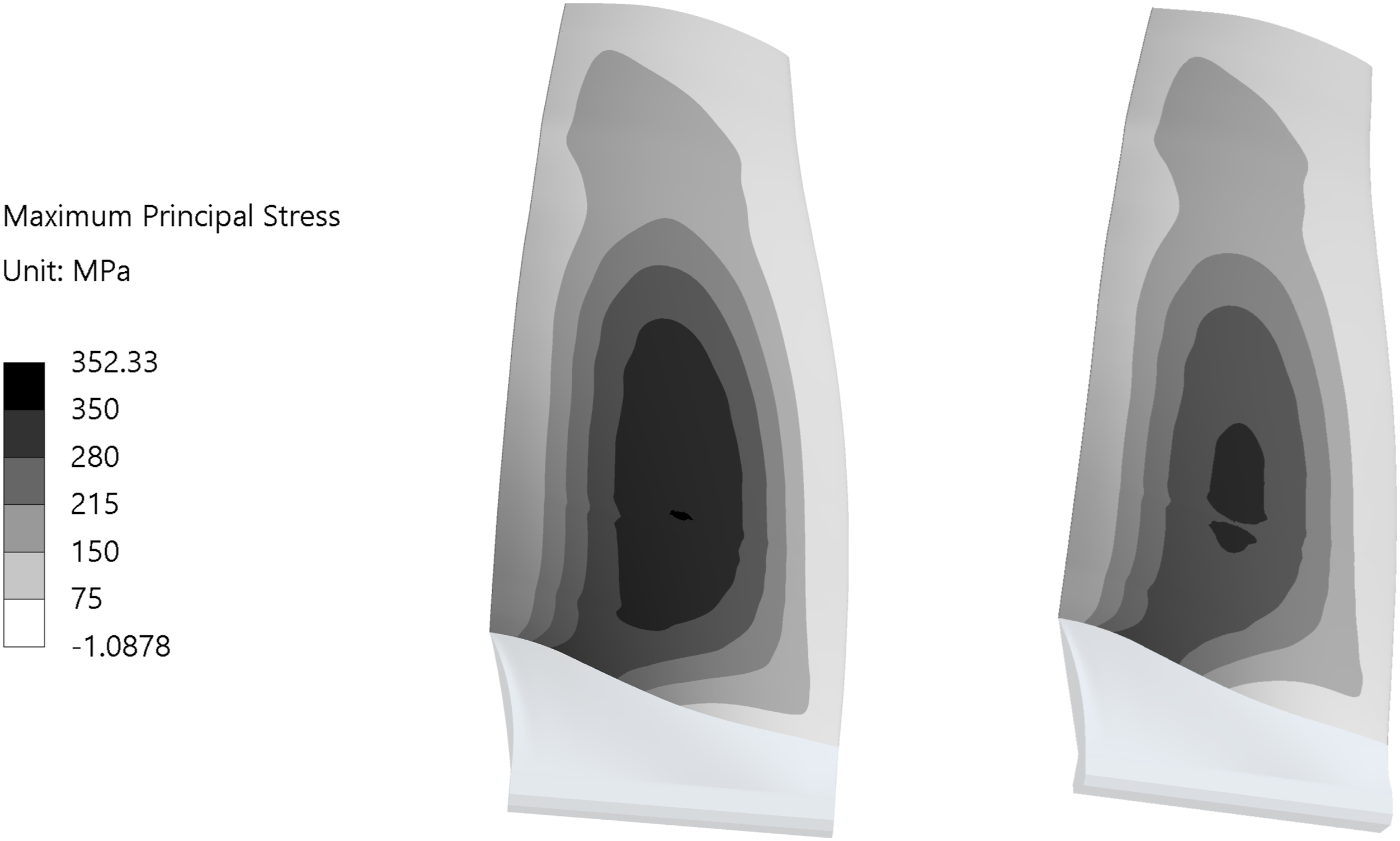

Similar to the results of the attaching the blade root analysis, these results also show that the consideration of the aerodynamic load leads to a similar stress distribution on the blade, but it has a high difference in value for the maximum stress, of approximately 15%. Though the difference is not as large as for the blade root inclusion analysis, it’s still considered large enough to be included in the analysis.

Because SimSolid does not allow mapping of the pressure distribution on the blade from CFD results, a comparison between the maximum stress results obtained with the mapping of the CFD pressure on the blade in Ansys Mechanical versus the stress results obtained by applying an equivalent integrated force on the blade in SimSolid was conducted on three geometries.

The three geometries were the VITAL datum blade and two additional geometries randomly selected from the design space that have visible large geometrical variations. All computations were done with the blade root attached, but the maximum stress of interest is on the blade, as the blade root is not being optimised, therefore the stress distribution comparison presented in Figure 7 only shows stress values on the blade surface, where the aerodynamic load is applied (top surface in Figure 4 (left), in light grey).

Figure 7.

Stress distribution on the fan blade computed with mapping the pressure distribution in Ansys Mechanical (right) versus applying an equivalent force in SimSolid (left) for three different geometries: (a) VITAL datum blade, (b) Geometry 1, (c) Geometry 2.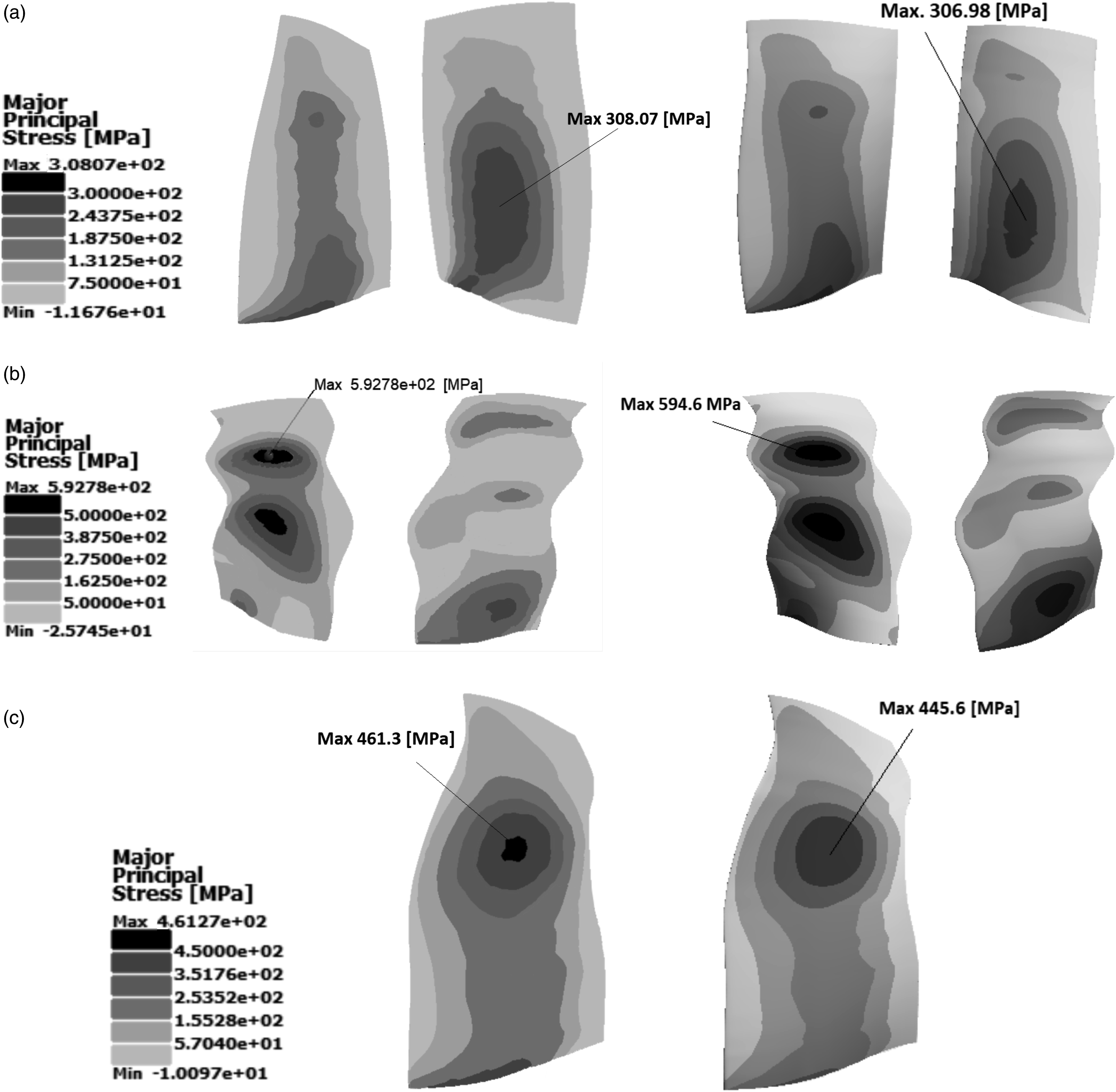

The results show that the relative difference between the two methods of computing the maximum stress is within 5% for all three geometries considered. Considering the computational time for a stress analysis is reduced by an order of magnitude using SimSolid, it was decided to proceed with SimSolid for the follow-on optimisation studies.

The material used for modelling the blade is a titanium alloy, with a yield strength value of 710 MPa.

For the computation of the maximum stress during the optimisation process, a response surface is created beforehand, applied to the same design space used in the optimisation process. Stress gradients are computed by a central finite-differencing. The relative step size for the finite difference approximation was kept to the default setting, for which a value is automatically selected.

Stress response surface generation and selection

This section details the generation and selection of the stress response surface method, according to the workflow diagram from Figure 8. For the maximum stress response-surface generation, three design-of-experiments (DoEs) were generated, based on the 35 design parameters described above. Since the aerodynamic load, computed by Hydra CFD, is considered in the structural model, the number of points in the VITAL fan blade DoE was limited, due to prohibitive computational costs of thousands of 3D CFD simulations.

Figure 8.

Stress response surface workflow diagram.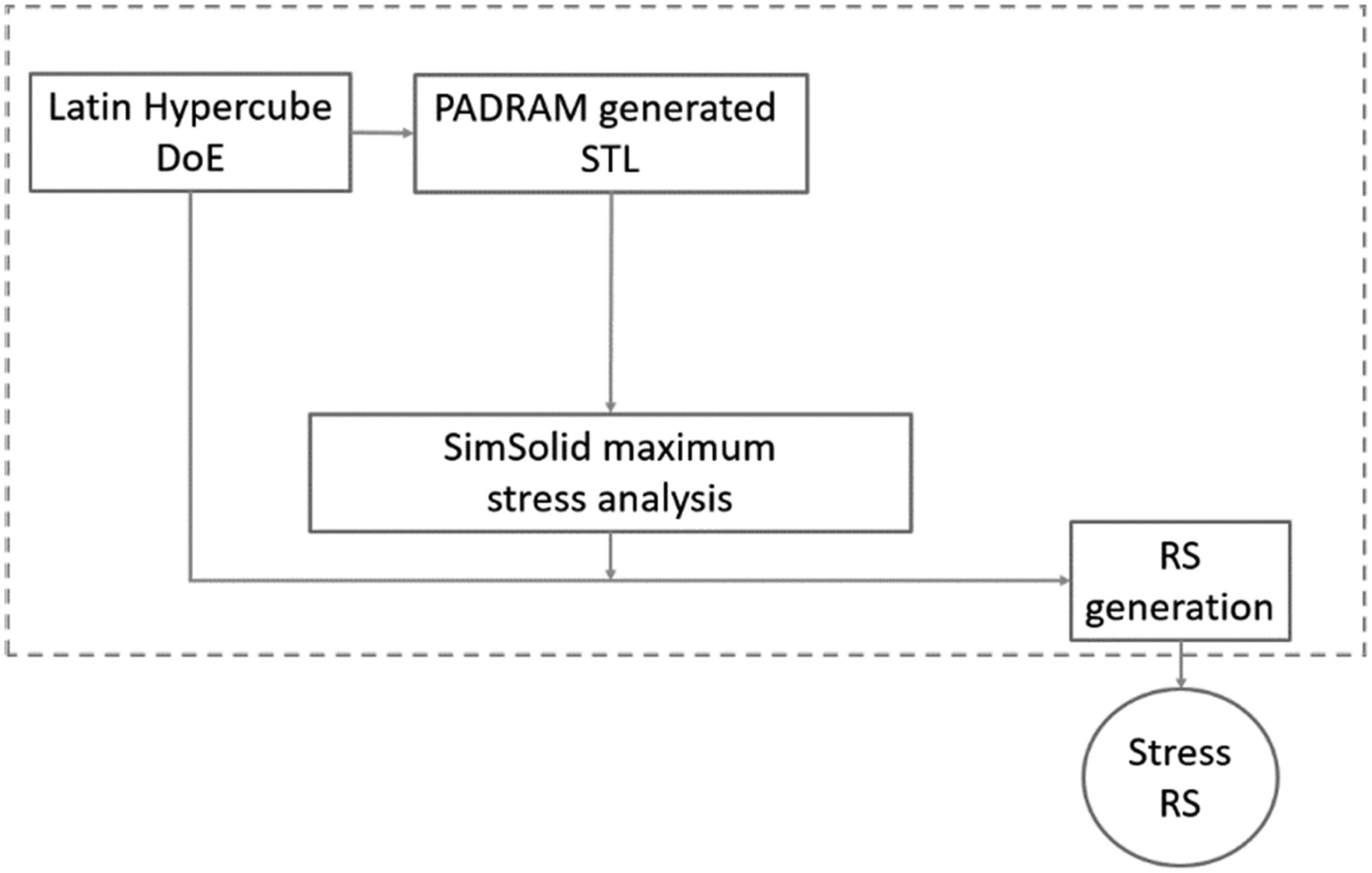

The initial VITAL fan blade DoE population consists of 610 runs. The sampling was done using Sobol’ sequences method, also called LPτ, because it provides good uniformity for high-dimensional problems even at a small number of sampled points.³¹ The targeted maximum stress constraint value for this fan blade is 500 MPa, to allow for a minimum safety factor of 1.4 compared to the yield strength of the material, which considers fatigue failure based on industrial experience.

Inspecting the values of the computed stress for the geometries generated, it emerged that very few points were created in the region of interest, set between 300 and 800 MPa. For this reason, an additional 290 points were created using the Latin Hypercube sampling method and added to the initial 610, resulting in a second DoE population made of 900 points. The Latin Hypercube sampling method³² was selected here due to the problem of spurious correlations in the higher dimension for the Sobol sampling technique.³³ Finally, to try further improving the points density and the response surface accuracy in the region of interest, an additional 1100 points were created by a separate Latin Hypercube sampling, for which the input ranges of the design parameters were limited to half the original values.

A sampling of 22 points from the region of interest, generated during an unconstrained optimisation process, was used for testing the accuracy of the response surfaces generating and selecting the best fit.

For each of the three DoEs, different response surface methods were tested, using the Rolls-Royce proprietary SOFT Optimisation library³⁴: Kriging, polynomial and radial basis functions (RBF). Only the Kriging results are reported here, as they provided better quality results for this application compared to the other 2 methods.

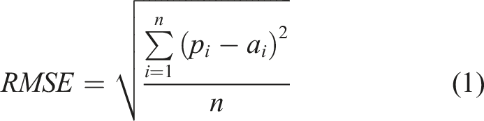
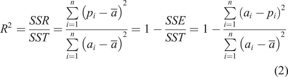
The computed stress values for the 22 test points are compared against the predicted values of the Kriging response surfaces based on the three DoEs in Figure 9. To quantify which of the model gives the best prediction, two parameters have been considered, the root mean square error (RMSE) and the coefficient of determination (R²). Both the RMSE and R² offer different, yet complementary, information.

Figure 9.

VITAL Computed stress values versus predicted stress values for the three DoEs.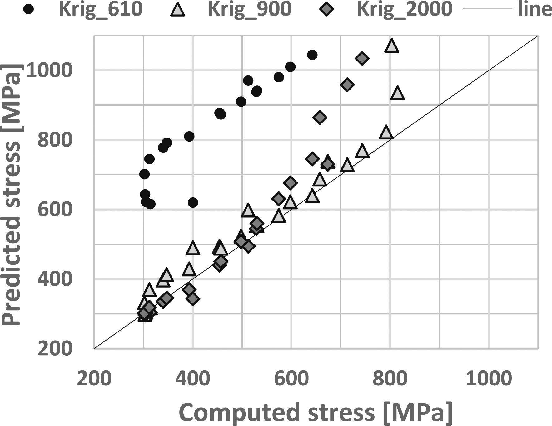

The Root-Mean-Square-Error (RMSE) measures the differences between values predicted by the model and the actual observed values. It is the average vertical distance of the actual data points from the fitted line. Smaller RMSE reflects greater accuracy. The RMSE is relatively easy to understand and communicate since reported values are in the same units as the dependant variable being modelled.

R M S E = \sqrt{\frac{\sum_{i = 1}^{n} {(p_{i} - a_{i})}^{2}}{n}}

(1)

where p is the predicted value, a is the actual value, i is the index and n is the total number of samples.

R² is a statistical measure that represents the proportion of the total variance in the observed data that can be explained by the model. It is a standardized measure of degree of fit, providing a measure of how well observed values are predicted by the model. It ranges from 0.0 to 1.0, with higher values indicating better agreement.

R^{2} = \frac{S S R}{S S T} = \frac{\sum_{i = 1}^{n} {(p_{i} - \bar{a})}^{2}}{\sum_{i = 1}^{n} {(a_{i} - \bar{a})}^{2}} = 1 - \frac{S S E}{S S T} = 1 - \frac{\sum_{i = 1}^{n} {(a_{i} - p_{i})}^{2}}{\sum_{i = 1}^{n} {(a_{i} - \bar{a})}^{2}}

(2)

where SST is the sum of squares total, SSR is the sum of squares explained by regression, SSE is the sum of squares error and

\bar{a}

denotes the average value.

Statistical texts frequently illustrate that R² is sensitive to outliers.³⁵ A model that can follow the observed data during extreme events, i.e., located far away from the others, will have an artificially higher value of R², which may obscure the true relationship between the predicted and observed data over most of the remainder of the domain.

Though the coefficient of determination shown in Figure 10 finds the 2,000 points DoE to be the best, the difference is very small compared to the 900 points based model. It is difficult to assess without additional tests whether a bias was introduced by considerably increasing the number of points, as the addition of the extra sampling points could have introduced outliers.

Figure 10.

VITAL maximum stress response surface comparison: Root mean square error (RMSE) (left) and coefficient of determination (R2) (right).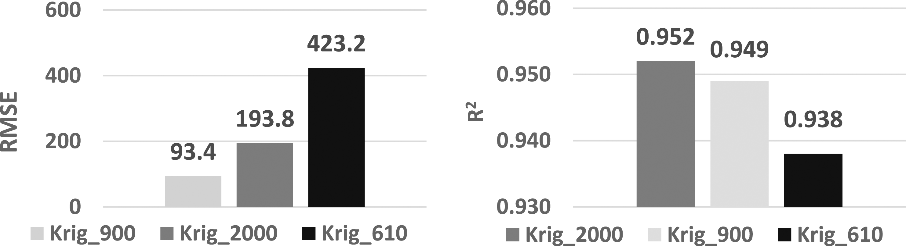

At the same time, the root mean square error (RMSE) values show that the 900 points DoE based response surface estimates have smaller differences from the computed values.

For the 2000 points-based response surface it can be seen in Figure 9 that the predicted stress values for the cases between 600 and 800 MPa are much larger than computed values, accounting for the higher value of the RMSE parameter. This is the region immediately above the stress value imposed as constrained, namely 500 MPa and, therefore, a region where increased accuracy is desired. Considering the aspects discussed above, the Kriging response surface based on 900 points was selected to proceed with as it has half the RMSE value, almost the same R² and better fit in the region around the constraint value.

Based on the above insight, further studies into improving the accuracy of the surrogate model can be made. First, a more judicious selection of the variation ranges of the design variables should precede the optimisation process. Secondly, state of the art sampling method that combine the advantages of both Latin Hypercube and Sobol’ sampling methods³⁶ should be used for designing the DoE. Last, but not least, novel surrogate models with increased accuracy for a low number of samples, such as neural network with active design subspaces should be considered for building the response surface.²³

Adjoint based multidisciplinary design optimisation

Aero-structural optimisation strategy

The workflow diagram for the stress constrained adjoint aerodynamic optimisation process is given in Figure 11. For the optimisation process, the Sequential Least SQuares Programming (SLSQP).³⁷ algorithm is used in this work.

Figure 11.

Aero structural optimisation workflow diagram.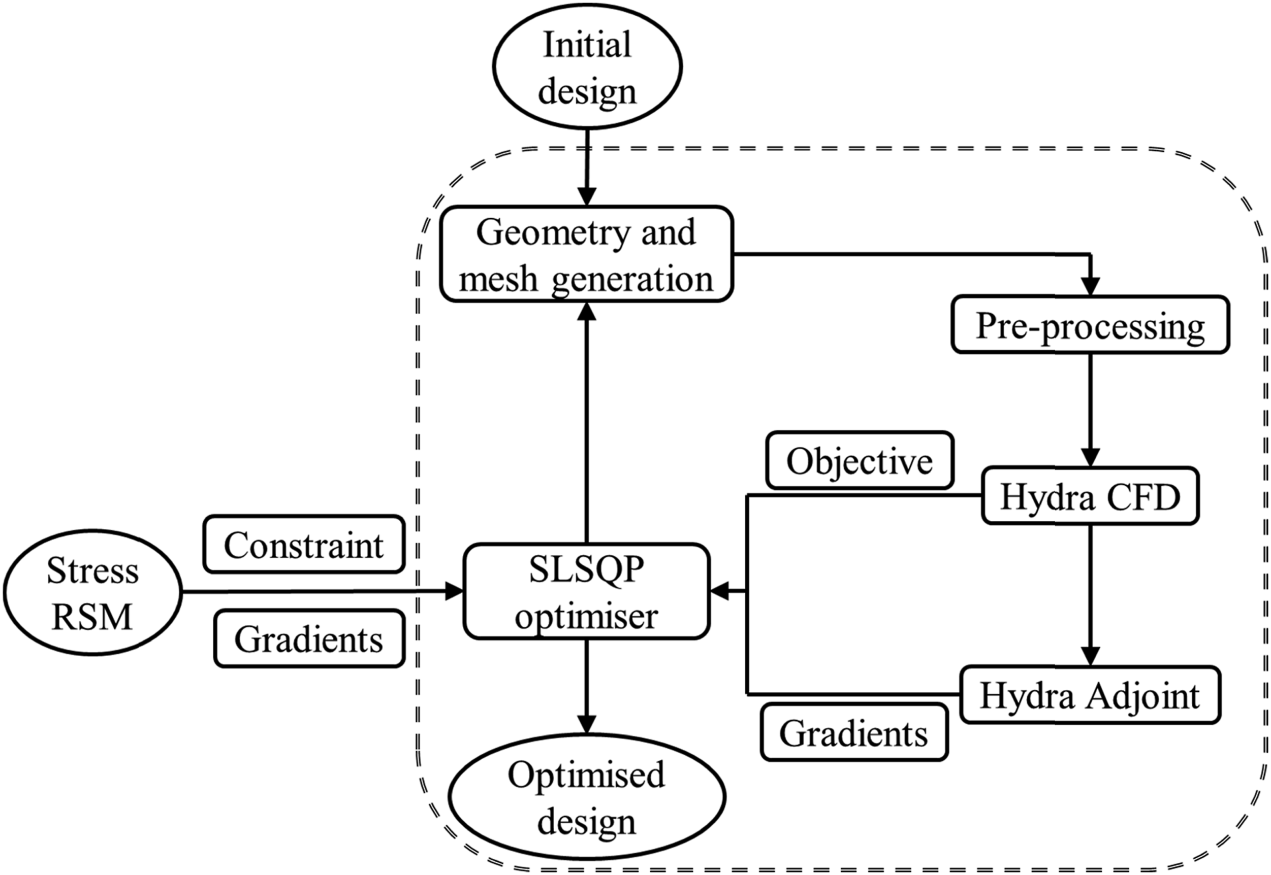

The process has as objective the maximization of the aerodynamic efficiency while constraining the maximum stress under a desired value. The aerodynamic computations were run to an exit capacity that fixes the required mass flow rate on the working line and the correct bypass ratio.

First, the stress response surface is generated separately, using the same design space and according to the workflow diagram presented in Figure 8. At the current step in the optimisation process, the geometry is generated and automatically meshed in PADRAM, based on the current set of 35 design parameters.

The CFD numerical computations are then conducted using Hydra to compute the aerodynamic efficiency and the gradient of the objective function is determined using its Adjoint. The maximum stress is also estimated using the response surface and the stress gradients are determined by finite difference. A feasible direction is obtained by solving the quadratic programming problem and using a line search to select the next design to be run. The process is repeated until the precision goal set for the value of the objective function is reached. In this case, the stopping criterion is obtaining a difference between the efficiency computed for two consecutive iterations below 1 × 10⁻⁴.

Aero-structural optimisation results

Based on the optimisation workflow presented in Figure 11 and the stress response surface presented in the previous section, one aerodynamic and two different aero structural optimisation processes were conducted for the VITAL fan blade. First optimisation was done without any stress constraint, for comparison purposes. Another optimisation was done with the stress constrained to the desired value, namely 500 MPa. Based on the test results obtained for the selected stress response surface presented in the previous section, it was observed that the actual stress could differ by as much as 25% from the estimated value. Therefore, a third optimisation process was run with the stress constrained set to 400 MPa, so that with this safety factor and the potential added 25% to still limit the actual stress value to 500 MPa.

The evolution of the efficiency (objective function) and maximum stress (constraint), for the three optimisation runs, is presented in Figure 12. The results show that the maximum stress was successfully constrained to the imposed values, but with a toll on the efficiency benefit, as compared to the unconstrained optimisation results.

Figure 12.

Unconstrained and stress constrained optimisation histories for: efficiency (left) and stress (right).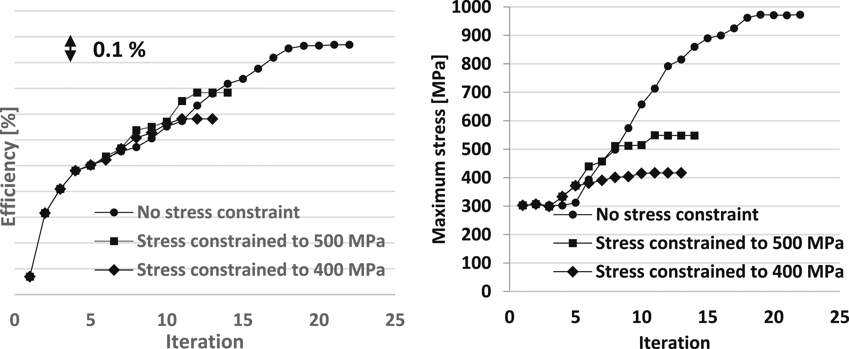

A summary of the optimisation results is given in Table 1. From this data, it can be seen that despite using a modern industrial fan blade considerable increase in efficiency is achieved in the unconstrained optimisation process. The efficiency benefit of the unconstrained optimisation is around 0.9%. This value is comparable with that obtained in a different optimisation process done for the same test case,²⁴ in which the authors reported a 0.8% increase in efficiency for the purely aerodynamic optimisation without any constraints and 0.76% increase in efficiency when the pressure ratio was constraint to maintain the design point for which the optimisation is done within 0.25%. The efficiency benefit obtained here is significant, as the datum geometry provided is already highly efficient. The efficiency benefit obtained here drops with the imposed stress constraint, first to 0.71% for 500 MPa and then to 0.61% for 400 MPa.

Table 1.

Fan blade aero mechanical optimisation results.

Geometry	Efficiency benefit (%)	Maximum stress [MPa)
Datum	—	302.8
Optimal with no stress constraint	0.9	972.8
Optimal with stress constrained to 500 MPa	0.71	548.0
Optimal with stress constrained to 400 MPa	0.61	416.7

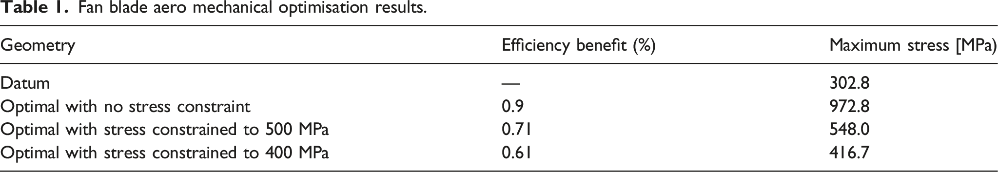
However, the maximum stress for the unconstrained case increases considerably as well, exceeding the desired 500 MPa, and reaching almost 1000 MPa. For the two stress constrained runs (500 MPa and 400 MPa), the stress reaches a predicted value of 548 MPa and 415.2 MPa. The actual computed stress distribution can be visualized in Figure 13 and the maximum stress values are about 25% higher than those produced from the response surface assessment. It can also be seen that the optimisation with the stress constraint set to 400 MPa successfully keeps the stress value close to the desired 500 MPa. For this reason, this run is considered to have produced an optimum geometry with the desired stress constraint and hence, is further analysed below.

Figure 13.

VITAL stress distribution comparison: (a) Datum, (b) Optimum with no stress constraint, (c) optimum with 500 MPa stress constraint, (d) Optimum with 400 MPa stress constraint.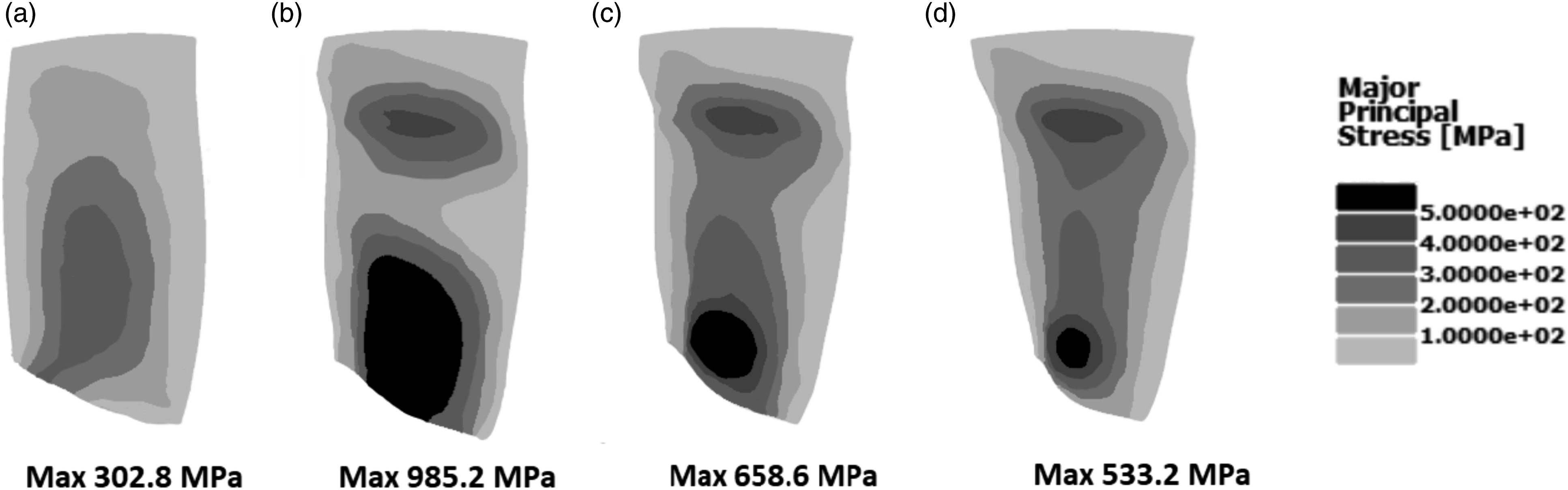

A comparison of the aerodynamic profiles is given in Figure 14, near the tip (left) and at mid-span (right).

Figure 14.

Aerodynamic profiles near tip (left) and at mid-span (right).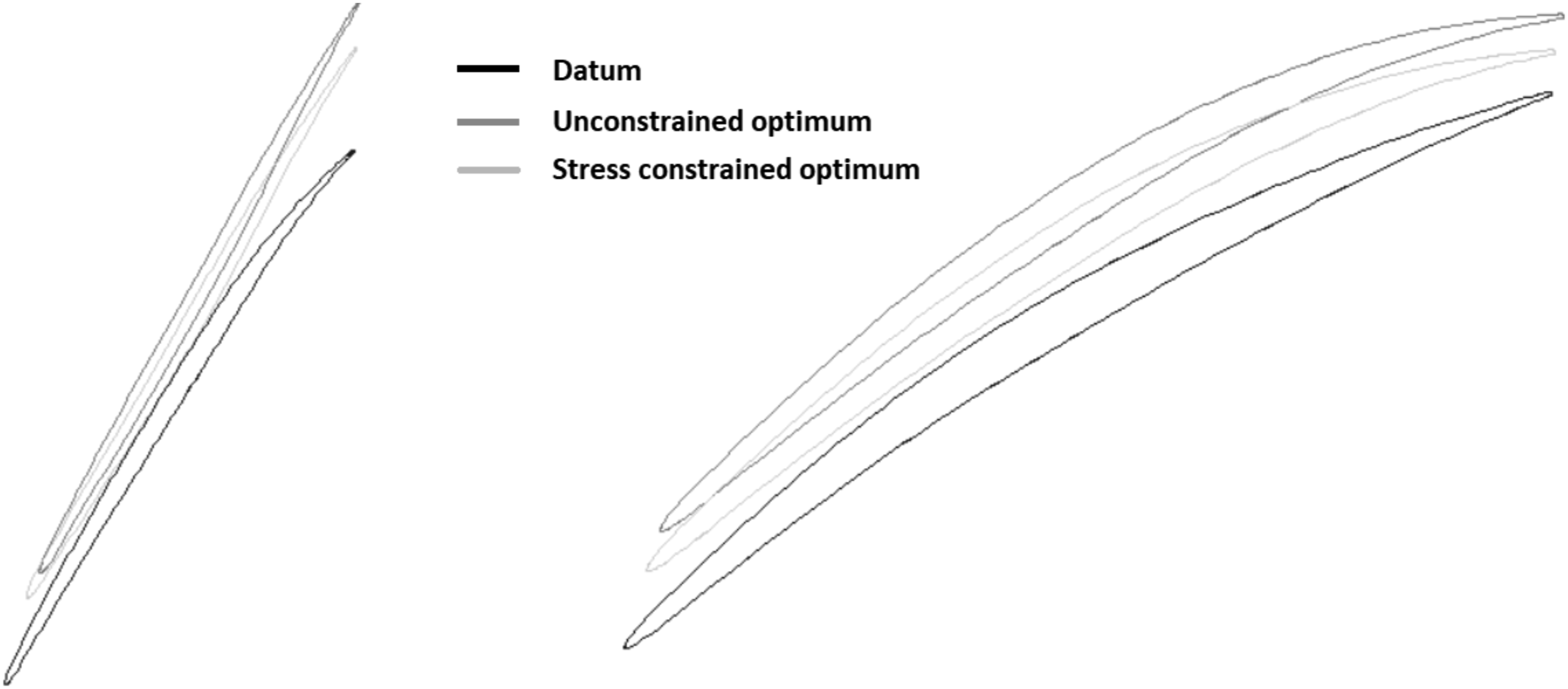

Near the tip, both unconstrained and constrained profiles have an S-shape camber line with negative camber in the front chord area and positive camber near the trailing edge. This is a result of the trailing edge recambering. The trailing edge opens for the optimal geometries compared to the datum, corresponding to a reduced stagger and increased throat area (blade “untwist”). However, at mid span the optimal geometries do not present the S-shape pattern. The major change in profile at this span is an increased camber close to the trailing edge, more pronounced for the unconstrained optimum.

Another distinctive feature with effect on the aerodynamic performance is the back sweep, larger near the tip and more pronounced for the unconstrained optimisation. Both optima also have a back lean with respect to the direction of rotation, with larger values for the unconstrained optimum, which impacts the maximum stress values. A comparison of the geometries in 3D can be visualized in Figure 15.

Figure 15.

3D comparison of the VITAL datum (black), unconstrained optimal geometry (dark grey) and stress constrained optimum (light grey).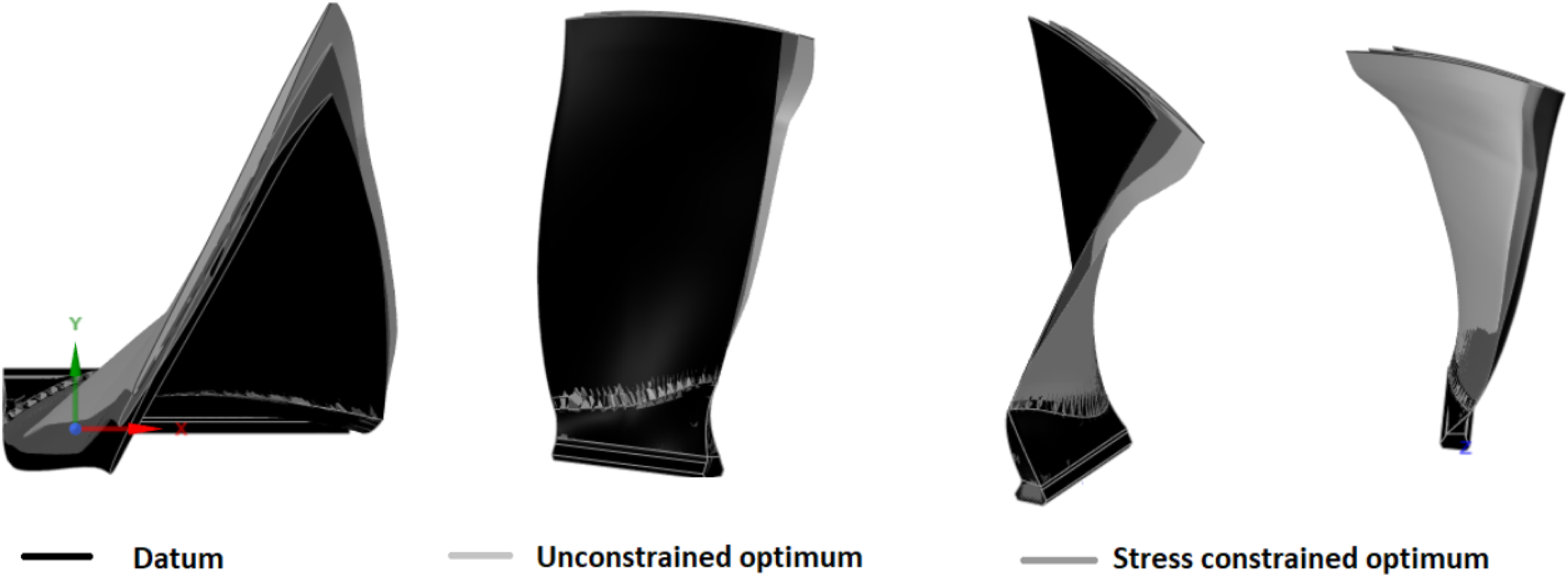

Figure 16 shows the pressure distribution on the blade for the datum and the two optimal geometries without and with stress constrained, while the separation regions are indicated by surfaces of zero axial velocity displayed in black. This figure reveals that the performance increase is realized in the upper 20% of the blade span, where both optimal designs weaken the shock and remove the shock induced separation.

Figure 16.

Pressure distribution on the VITAL blade: (a) datum, (b) unconstrained optimum, (c) stress constrained optimum.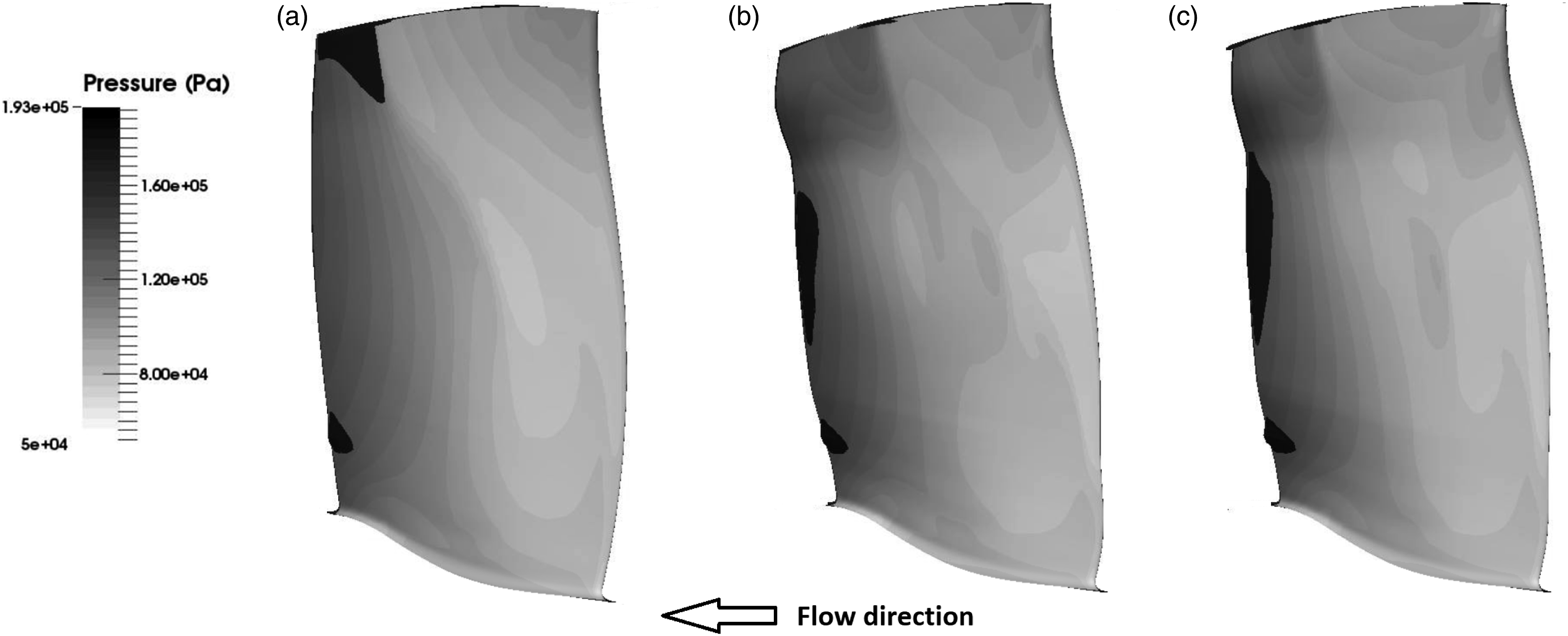

Figure 17 gives a clear picture of the shock wave pattern in the near tip region. The Mach number distribution for the datum geometry shows the bow shock wave detached from the blade leading edge and the passage shock being formed by a bow-wave portion and a strong normal shock on the suction surface of the adjacent blade.

Figure 17.

Mach number distribution on the VITAL blade near the tip (95% span) for: (a) datum, (b) unconstrained optimum; (c) stress constrained optimum.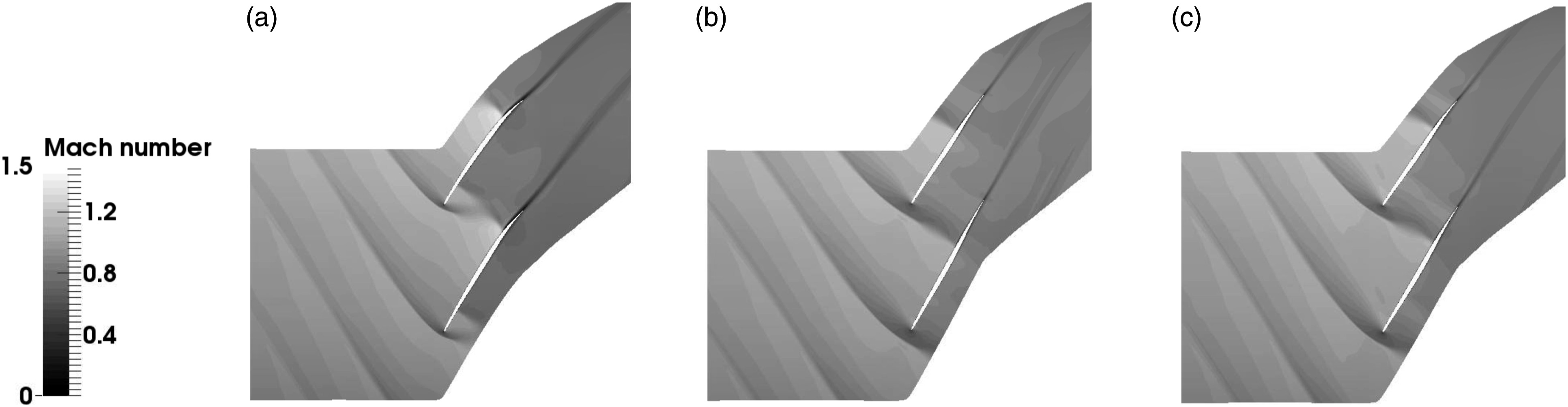

The purely aerodynamic optimised geometry improves the efficiency mainly by reducing the peak Mach number before the shock wave in the near tip region. This is of primary importance due to the strongly rising pressure losses with increasing pre-shock Mach number and shock induced separation. This is mitigated by the recambering of the blade profiles in the near tip region. The reduction of the pre-shock Mach number is achieved by the S-shape of the aerofoil which has negative curvature in the front part of the blade suction side which leads to a pre-compression reducing the Mach number upstream of the final strong shock.

For the mid span region, a slight increase in pressure losses is noticeable for both optimal geometries, due to flow separation introduced at the blade trailing edge, which is a direct consequence of the increased local camber. This is visible in the distribution of the Mach number at mid-span plotted in Figure 18.

Figure 18.

Mach number distribution at design point on the VITAL blade at mid-span for: (a) datum, (b) unconstrained optimum; (c) stress constrained optimum.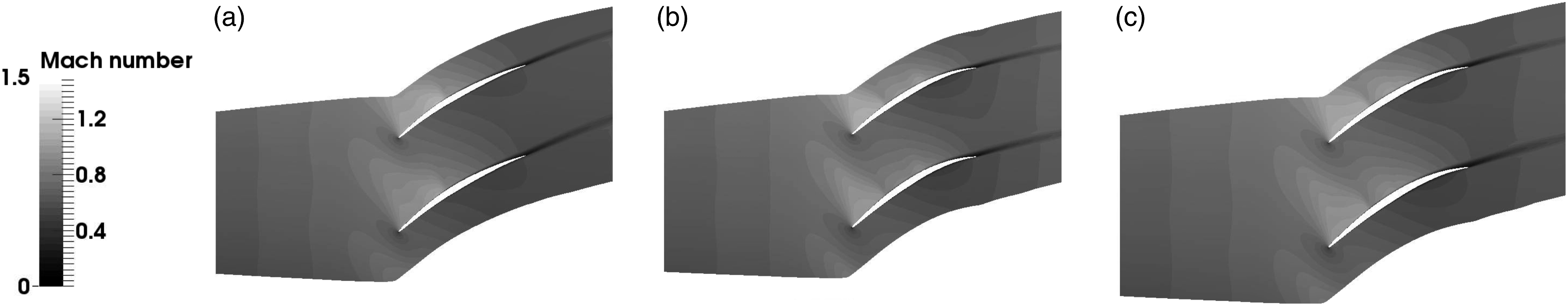

At the same time, the back-sweep present near the tip moves the shock wave out of the passage. Figure 17 b and c exhibit the bow shock completely detached from the leading edge.

Hah et al.³⁸ have numerically and experimentally shown that back sweep causes a reduction in stall margin while forward sweep leads to improved stability. Blaha et al.³⁹ further consolidated this conclusion with numerical and experimental studies on the performances of back swept transonic compressor rotor while Passrucker et al.⁴⁰ for the forward swept transonic rotors. To assess the aerodynamic performance at off design conditions, numerical simulations for different mass flow rates were also computed for the VITAL fan. The efficiency is pictured in Figure 19 (left) and the pressure ratio in Figure 19 (right), for the three geometries: datum, unconstrained optimum and stress constrained optimum.

Figure 19.

Total rotor efficiency (left) and total pressure ratio (right) for the VITAL fan.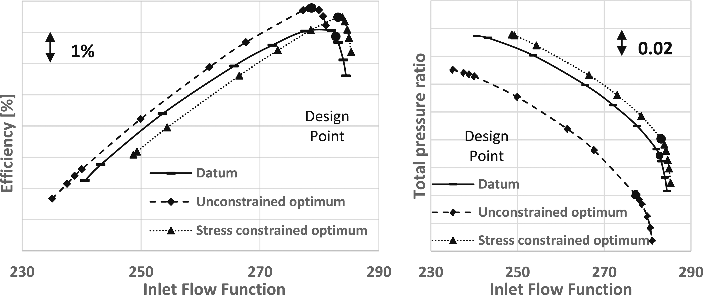

The unconstrained optimum has better efficiency for all computed points and maintains good stability margin, but the pressure ratio drops considerably, by approximately 2.2% for the design point. This means that the design point must be recovered through other means, adding to the required design effort and risking losing the potential efficiency benefit.

The stress constrained optimum has higher efficiency in the region of the design point, but the efficiency is slightly lower for lower mass flow rates. At the same time, this geometry has a reduced stability margin. The predominant geometrical feature responsible for this is the backward sweep, which impacts the blade loading and the shock position.

Denton and Xu⁴¹ showed that, because the pressure gradient perpendicular to a plane end wall must be zero, the blade loading near the upper wall must be increased near the leading edge since there can be little pressure difference between it and the more highly loaded region below it. The back sweep diverts the flow away from the blade tip region which destabilizes the region.

Due to the presence of the casing end wall, the spanwise shock shape does not follow the sweep direction but moves normal to the casing in the proximity of the tip, which causes the shock wave to move upstream of the leading edge and becomes normal to the incoming flow which leads to a higher flow incidence and, thus to a reduced stall margin.

Overall, the effect of sweep on the stall margin of both optimal geometries is similar, though not directly visible for the unconstrained one. For this geometry, the pressure ratio has been reduced considerably. To recover from this, the fan would need to operate at higher speed, for the same mass flow rate which, in turn, leads to a considerable reduction of the stall margin. By comparison, for the stressed constrained optimum, the pressure ratio increases for all computed points, with an average of 0.55%. This shows the potential to operate at a lower speed, which may lead to further efficiency increase and to an improvement of the stability limit.

Figure 20 shows the contours of relative Mach number at mid-span and near tip (95% of the span) for the three geometries of interest, datum, unconstrained optimum and stress constrained optimum. Compared to the design point distributions shown in Figure 18, there is little difference at mid-span. Near the tip, the passage shock moves further away from the leading edge for all three geometries and forms a stronger detached shock. Since shock-impingement position of detached shock is located ahead of the change in tip profile between the different geometries, the flow field characteristics upstream of the detached shock for all three rotor blades are almost the same. The separation induced by the shock wave also strengthens visibly in the passage, with large low velocity regions appearing in the tip region. This is consistent with the key stall inception mechanism of highly loaded transonic rotors. The change in the near tip profile camber between mid-chord and trailing edge for the stress constrained optimum results in a reduced boundary layer separation.

Figure 20.

Mach number distribution near stall on the VITAL blade at near tip (up) and mid-span (down) for: (a) datum, (b) unconstrained optimum; (c) stress constrained optimum.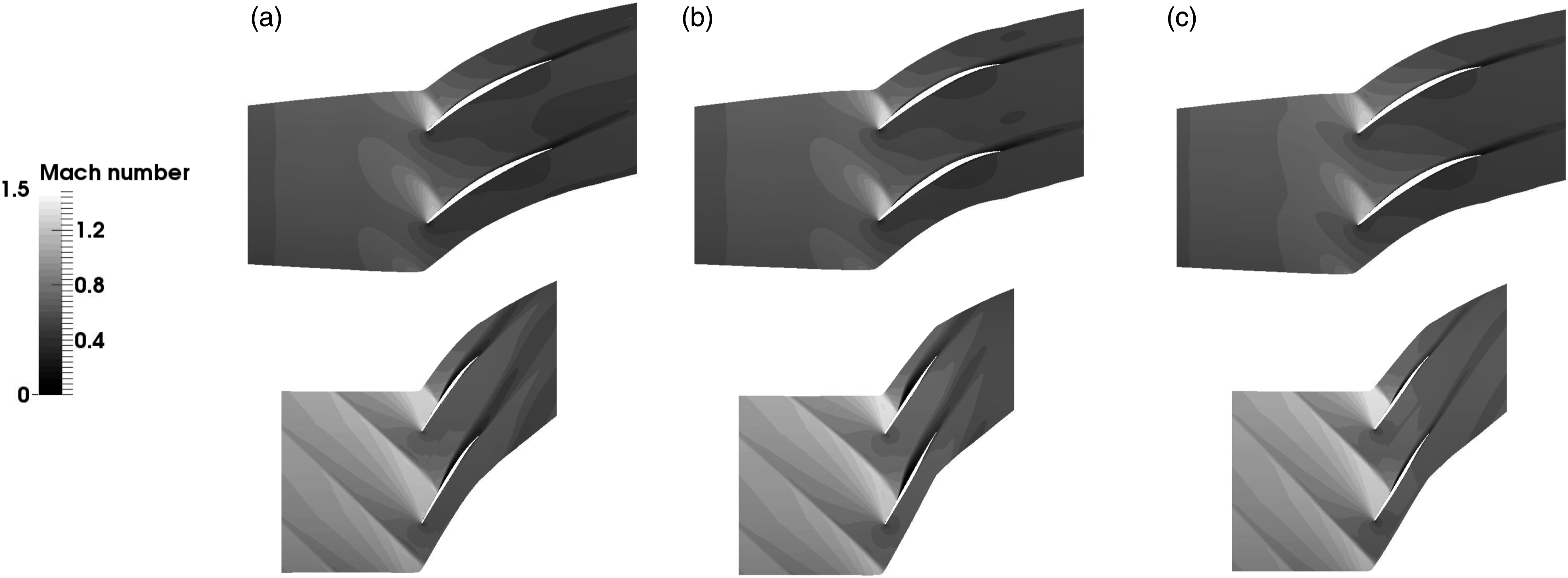

Flutter computations

The aeroelastic instability of flutter continues to affect the safety and reliability of turbomachinery. This occurs when the unsteady work performed by the fluid on the blade leads to self-excited oscillation that exceed the energy dissipated by damping in the system. Specifically, the aerodynamic damping plays a very significant role in the flutter analysis of modern rotors.

Due to the unsteady nature of this phenomenon, the existing numerical methods for flutter prediction are still very computationally expensive, and difficult to implement into an MDO process, whether is fully coupled fluid-structure interaction or response surface method. For this reason, flutter computations were carried out here as a verification of the datum and optimised fan blade geometry for evaluation.

The aerodynamic design geometry of the fan blade is the “hot” (running) shape. For aeroelastic predictions, such as flutter analysis, the “cold” geometry is needed to perform the pre-stress modal analysis. The results of the modal analysis, namely the vibration frequencies and modes will then serve as input in the flutter analysis. To obtain the cold geometry from the hot geometry, an iterative process is employed, as described in Figure 21.

Figure 21.

Hot-to-cold geometry process.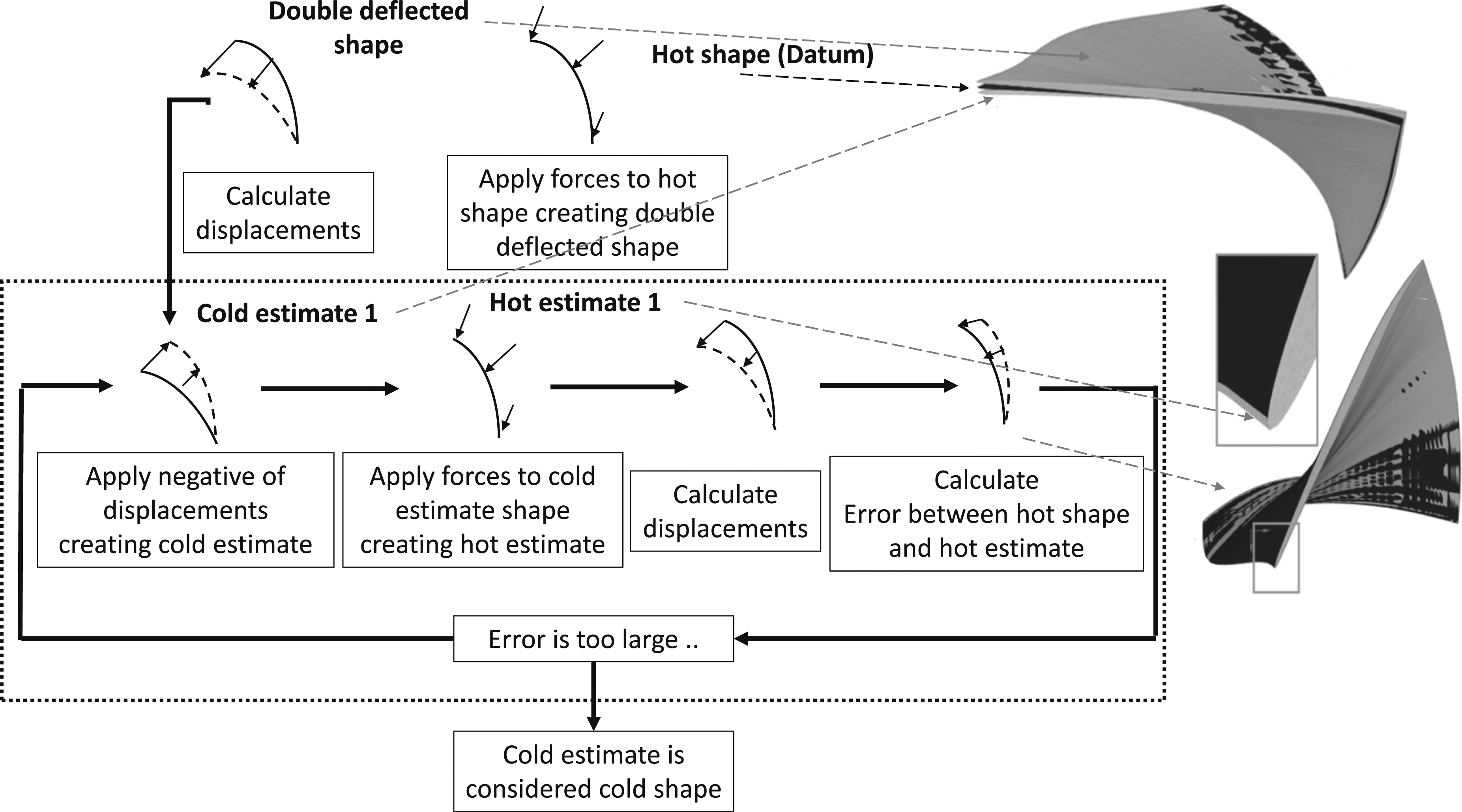

It comprises the following major steps:

- Apply forces to hot shape an create the “double deflected” shape

- Compute the displacement

- Subtract the displacements from the hot shape and create the cold shape estimate

- Apply forces to the cold estimate and obtain the hot estimate

- Compare the hot estimate with the datum (the hot shape)

- Repeat the process starting with the hot estimate until the errors are within acceptable limits.

Damping computations require as input the natural frequency of the blade (vibration mode frequency) and the blade displacements (mode shapes). The flow is solved over vibrating blades with these prescribed blade frequency and displacements.

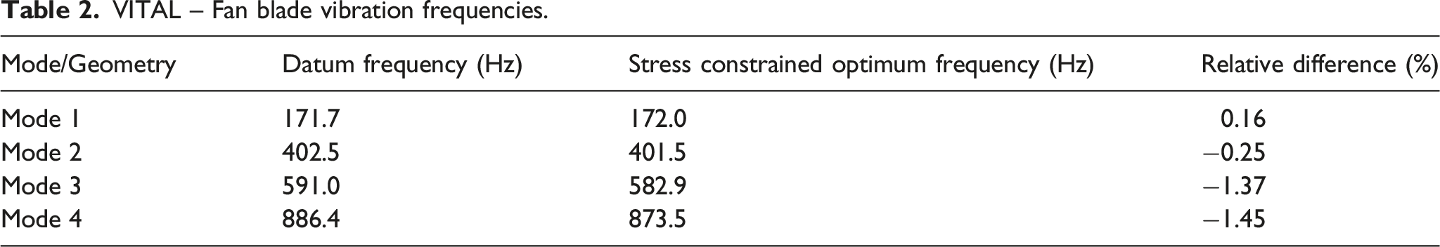
A pre-stressed modal analysis needs to be performed to determine the blade natural frequencies and mode shapes, in which the centrifugal and aerodynamic loads are applied to the cold flow geometry. A rotor consists of many modes, but only the first three or four usually contribute to flutter and are considered during a blade flutter simulation. A comparison of the vibration frequencies computed for the Vital datum and for the stress constrained optimised geometry is given in Table 2. It can be seen that for the first four vibration modes, the relative difference between the natural frequencies of the datum geometry versus the stress constrained optimum is under 1.5%.

Table 2.

VITAL – Fan blade vibration frequencies.

Mode/Geometry	Datum frequency (Hz)	Stress constrained optimum frequency (Hz)	Relative difference (%)
Mode 1	171.7	172.0	0.16
Mode 2	402.5	401.5	−0.25
Mode 3	591.0	582.9	−1.37
Mode 4	886.4	873.5	−1.45

The energy method based on traveling wave model assumption developed by Lane⁴² to predict whether flutter happens is generally used in turbomachinery for flutter predictions. This model is based on the blade vibration being modelled as periodic motion at fixed frequency with a specified phase angle. The deformation is repeated periodically around the rotor according to the phase angle multiplier.

For the Vital case, the selected vibration amplitude is 1.5 mm, just under 1% of the tip chord, and the imposed mode shape, representing the first mode of vibration, can be visualized in Figure 22, for the datum (left) and for the stress constrained optimum geometry (right).

Figure 22.

VITAL (a) Datum and (b) stress constrained optimum blades first vibration mode shapes.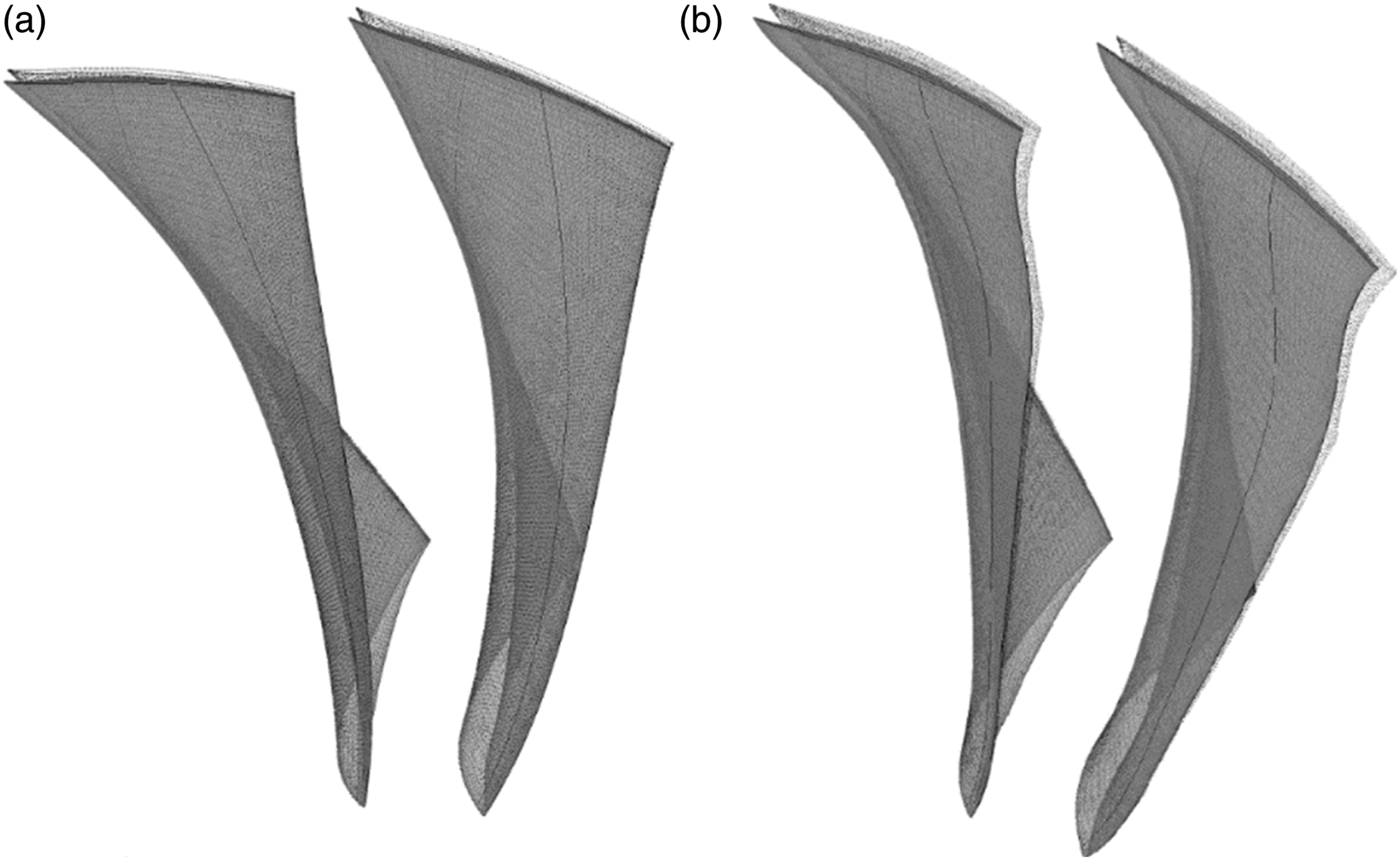

For a rotor consisting of N blades, there is a finite number of disc nodal diameters. At nodal diameter ND = 0, all the blades vibrate in phase with an Interblade Phase Angle (IBPA) of 0. However, for other nodal diameters, each blade will be out of phase with respect to the others by a finite interblade phase angle value. The interblade phase angle can be computed from the nodal diameter as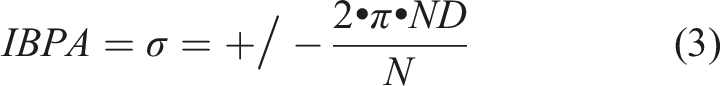

I B P A = σ = + / - \frac{2 ∙ π ∙ N D}{N}

(3)

where 0 ≤ ND ≤ N/2 for an even number of blades and 0 ≤ ND≤(N-1)/2 for an odd number of blades. The positive sign of ND means the motion direction of traveling wave is the same as fan rotation direction (forward), and negative sign means opposite direction of travel (backward).

The main objective of a blade flutter analysis is to obtain the aerodynamic damping, or work per vibration cycle. This calculation yields a measure of the system stability at each nodal diameter and blade vibration frequency. The work per vibration cycle can be computed as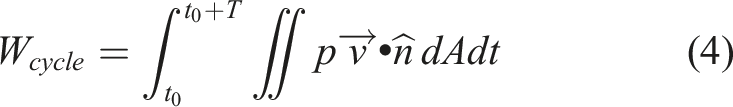

W_{c y c l e} = \int_{t_{0}}^{t_{0} + T} \iint p \vec{v} ∙ \hat{n} d A d t

(4)

where: T = 2π/ω (the period of one vibration cycle), t₀ is the time at the start of the vibration cycle, ω is the vibration frequency, p is the fluid pressure, v is the velocity of the blade due to imposed vibrational displacements, A is the surface area (in this case, the surface of the blade),

\hat{n}

is the surface normal unit vector.

Positive values for work indicate that the vibration is damped (for the frequency being studied), whereas negative values indicate that the vibration is undamped.

The aerodynamic damping results for the first mode of vibration at design speed for the Vital datum geometry and for the stress constrained optimal geometry are given in Figure 23.

Figure 23.

VITAL Datum and stress constrained optimum aerodynamic dumping ratio for the first vibration mode.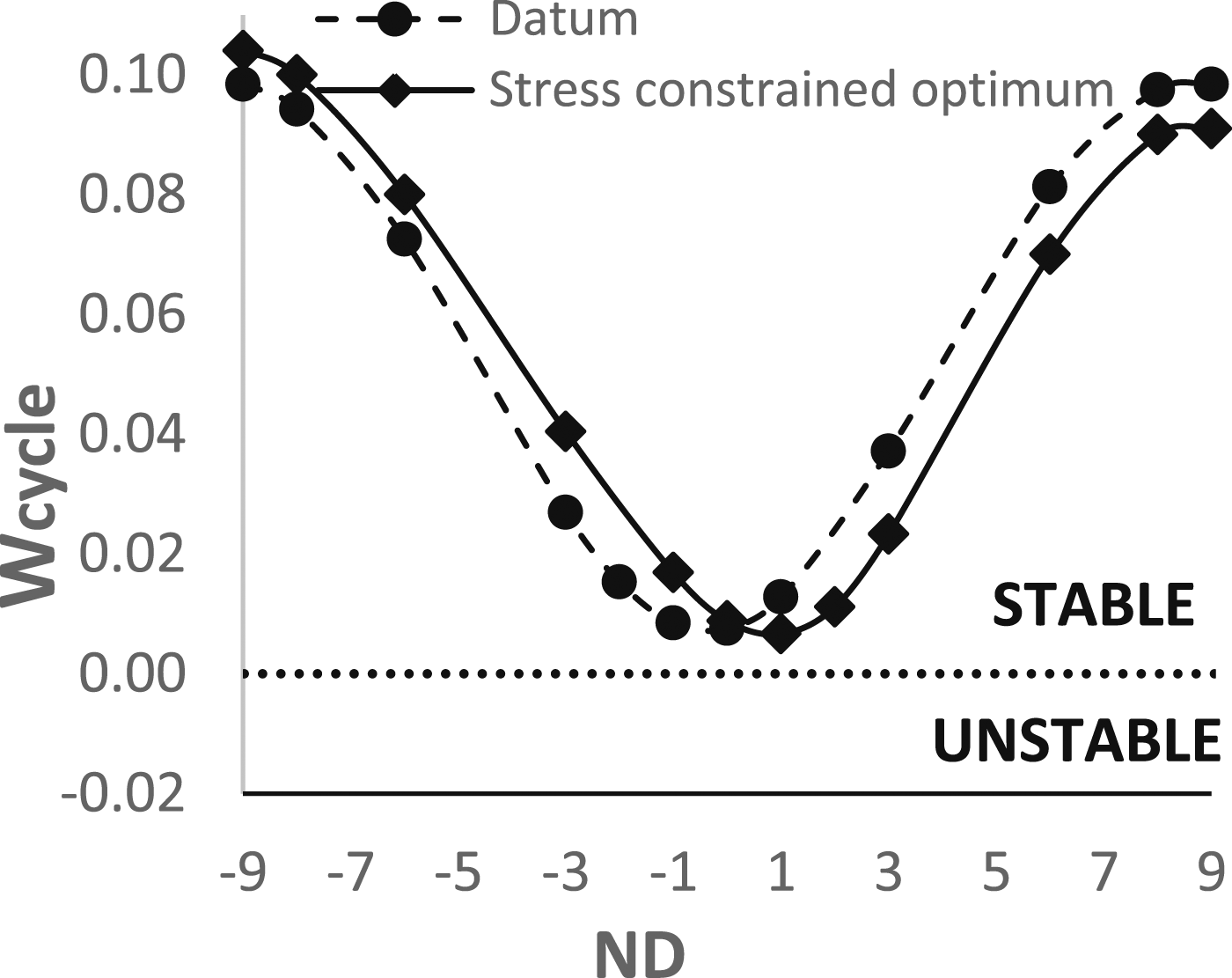

It can be observed that the two curves are very similar, with a slight shift in nodal diameter for the optimal geometry but maintaining stability for all nodal diameters. For the datum geometry, according to existing experimental data, flutter is not expected at the design point, which is confirmed by these results. Based on this flutter evaluation for the stress constrained optimal geometry, the optimised blade shows a similar flutter behaviour, without any stability degradation.

Conclusion

A novel method is presented that combines an adjoint based high-fidelity aerodynamic optimisation with a response surface-based stress constraint applied to a modern low-pressure fan blade. The results highlight the importance of using a multidisciplinary approach in the optimisation process (CAD-CFD-FEA), as the stress can increase drastically if it is not constrained.

The method successfully leads to the increase in aerodynamic efficiency by 0.6% for the VITAL fan blades, while maintaining the stress below 500 MPa and increasing the pressure ratio by 0.5%.

Different geometric features have been identified that affects the aerodynamic and structural performances. The blade sweep and profile leading edge recambering affect mainly the aerodynamic performances, while the maximum stress values are mostly affected by the blade lean and thickness.

The aerodynamic loss reduction obtained with the optimal shape is the result of profile recambering of the near tip profiles, leading to a novel S-shape blade with negative camber close to the leading edge and positive camber near the trailing edge region. This shape reduces the peak Mach number before the shock wave in the near tip region, cutting down on the shock induced total pressure loss.

From a structural standpoint, the blade lean causes the stress at the base of the blade to increase by producing a bending moment due to the tangential component of the centrifugal force, which in turn leads to a local increase of the equivalent stress. The blade sweep variations along the span and leading edge recambering can also introduce local stress concentrators. For this reason, all the geometrical features have been observed to be less pronounced for the stress constrained optimal geometry as compared to the purely aerodynamic optimum.

The stall margin is also affected by the optimisation process. The main feature leading to poor stability margin is the back sweep of the blade which leads to an increased load in the tip region and to a movement of the shock upstream of the leading edge, causing an increase in flow incidence. Flutter verification computations showed that the optimised blade has a similar flutter behaviour for the design point, without any stability degradation.

Footnotes

Acknowledgments

The authors acknowledge Rolls-Royce’s support for the computing facility and software used in this work and for the permission to publish the work.

Declaration of conflicting interests

The author(s) declared no potential conflicts of interest with respect to the research, authorship, and/or publication of this article.

Funding

The author(s) disclosed receipt of the following financial support for the research, authorship, and/or publication of this article: This work is funded by the MADELEINE project from the European Union’s Horizon 2020 research and innovation programme under grant agreement No. 769025.

ORCID iD

Cleopatra Cuciumita

References

Zheng

. Review of design optimization methods for turbomachinery aerodynamics. Pro Aero Sci 2017; 93: 1–23.

Walter

William

Donald

. Design and performance of a 427-meter-per-second-tip-speed two-stage fan having a 2.40 pressure ratio. NASA TP-1314 October 1978.

Heidelberg

. Fan noise source diagnostic test-tone modal structure results. In: AIAA Paper No. 2002-2428, 8th AIAA/CEAS Aeroacoustics Conf, Breckenridge, Colorado, 2002.

Pazireh

Defoe

. A new loss generation body force model for fan/compressor blade rows: application to uniform and non-uniform inflow in rotor 67. J Turbomach 2022; 144(6): 1–41.

Xue

. Engineering application of an identification method to shock-induced vortex stability in the transonic axial fan rotor. Int J Aero Eng 2021; 2021: 1–24.

Fiore

Daroukh

Montagnac

. Loss assessment of the NASA source diagnostic test configuration using URANS with phase-lagged assumption. J Turbomach 2022; 144(no. 5): 1–12.

Kholodov

Moreau

. Identification of noise sources in a realistic turbofan rotor using large eddy simulation. Acoustics 2020; 2(no. 3): 691–706.

Lewis

de Laborderie

Sanjosé

, et al. Parametric study on state-of-the-art analytical models for fan broadband interaction noise predictions. J Sound Vibra 2021; 514: 116423–116428.

Grace

Gonzalez-Martino

Casalino

. Analysis of fan-stage gap-flow data to inform simulation of fan broadband noise. Phil Trans R Soc A 2019; 377: 1–19.

10.

Oyama

Liou

Obayashi

. Transonic axial-flow blade shape optimization using evolutionary algorithm and three-dimensional Navier-Stokes solver. In: 9th AIAA/ISSMO Symposium on multidisciplinary Analysis and optimization, Atlanta: Georgia, 2002. AIAA 2002-5642.

11.

Zheng

Xiang

Sun

. “Blade geometry optimization for axial flow compressor”. In: proceedings of the ASME turbo expo 2010: power for land, sea and air, GT2010-22229, Glasgow, UK, 2010.

12.

Lian

Liou

. Multiobjective optimization using coupled response surface model and evolutionary algorithm. AIAA J 2005; 43(No. 6): 1316–1325.

13.

Lian

Liou

. Aerostructural optimization of a transonic compressor rotor, J Propul Power 2006; 22(4): 880–888.

14.

Pierret

Filomeno Coelho

Kato

. Multidisciplinary and multiple operating points shape optimization of three-dimensional compressor blades, Struct Multidiscipl Optim 2006; 33: 61–70.

15.

Jameson

Martinelli

Pierce

. Optimum aerodynamic design using the navier-stokes equations. Theor Comput Fluid Dyn 1998; 10: 213–237.

16.

Carini

Blondeau

Fabbiane

, et al. Towards industrial aero-structural aircraft optimization via coupled-adjoint derivatives. In: AIAA Aviation 2021 Forum, 2021. AIAA. Virtual.

17.

Verstraete

Müller

. “Multidisciplinary adjoint optimization of turbomachinery components including aerodynamic and stress performance”. In: 35th AIAA Applied Aerodynamics Conference, Denver, Colorado, USA, 2017. AIAA Paper No. AIAA 2017-4083.

18.

Müller

Verstraete

Schwalbach

. Adjoint-based multidisciplinary, multipoint optimization of a radial turbine considering aerodynamic and structural performances. In: Proceedings of the ASME Turbo Expo 2019: Turbomachinery Technical Conference and Exposition, Phoenix, Arizona, USA, 2019. ASME Paper No. pp. GT2019–91823.

19.

Trompoukis

Tsiakas

Asouti

, et al. Continuous adjoint shape optimization of internally cooled turbine blade. Int J Turbomach Propuls Power 2021; 6(2): 20.

20.

Luo

Zhou

Liu

. Multipoint design optimization of a transonic compressor blade by using an adjoint method. ASME J Turbomach 2014: 136(5): 1–10.

21.

John

Qin

Shahpar

. The influence of parameterisation setup on the constrained adjoint optimisation of transonic fan blades. In: Proceedings of ASME Turbo Expo 2020: Turbomachinery Technical Conference and Exposition, 2020. GT2020-15352, Virtual.

22.

Giugno

Shahpar

Traverso

. Adjoint-based optimization of a modern jet-engine fan blade. In: Proceedings of the ASME Turbo Expo 2020: Turbomachinery Technical Conference and Exposition, 2020; Volume 2D. Turbomachinery, Virtual.

23.

Lopez

Ghisu

Shahpar

. Global optimisation of a transonic fan blade through AI-enabled active aubspaces. In: Proceedings of the ASME Turbo Expo 2021: Turbomachinery Technical Conference and Exposition, 2021. GT2021–59166, Virtual.

24.

Wilson

Kim

, et al. “Low-noise blade design optimization for a transonic fan using adjoint-based MDO approach”. In: AIAA Aviation 2021 Forum, 2021. AIAA 2021-3055, Virtual.

25.

Chicane

. “Multidisciplinary design optimisation of aero-engine fan blades”. Ph.D. dissertation. UK: University of Cambridge, 2018.

26.

Lapworth

. Hydra-CFD: a framework for collaborative CFD development. In: International Conference on Scientific and Engineering Computation (IC-SEC), Singapore, 2004. Vol. 30.

27.

Giles

Duta

Muller

, et al. Algorithm developments for discrete adjoint methods. AIAA J 2003; 41(no. 2): 198–205.

28.

Shahpar

Lapworth

. PADRAM: parametric design and rapid meshing system for turbomachinery optimisation. In: Proceedings of the ASME Turbo Expo 2003: Turbomachinery Technical Conference and Exposition, Atlanta, Georgia, USA, 2003. ASME Paper No. GT2003–38698.

29.

SIMSOLID . “SIMSOLID technology overview”. Whitepaper, 2015, pp. 1–21.

30.

Apanovitch

. “The method of external finite element approximations”. Minsk 1991. ISBN 5-339-00597-6.

31.

Sobol

Asotsky

Kreinin

, et al. Construction and comparison of high-dimensional Sobol’ generators. Wilmott 2011; 2011: 64–79.

32.

Iman

. Latin Hypercube Sampling. Wiley Online Library, 2008. DOI: 10.1002/9780470061596.RISK0299

33.

Chi

Beerli

Evans

, et al. On the scrambled soboĺ sequence. In: Sunderam

van Albada

Sloot

PMA

, et al. (eds) Computational Science – ICCS 2005, Lecture notes in computer science, vol. 3516. Berlin, Heidelberg: Springer, 2005. DOI: 10.1007/11428862_105

34.

Shahpar

. SOFT: a new design and optimisation tool for turbomachinery. In: Proceedings of Evolutionary Methods for Design, Optimisation and Control, CIMNE, Athens, 2002.

35.

Moore

. Statistics: concepts and controversies. 3rd ed. New York: W. H. Freeman, 1991, p. 439.

36.

Dige

Diwekar

. Efficient sampling algorithm for large-scale optimization under uncertainty problems. Comput & Chemic Eng 2018; 115: 431–454.

37.

Oliphant

. Python for scientific computing. Comput Sci Eng 2007; 9(no. 3): 10–20.

. Control of shock structure and secondary flow field inside transonic compressor rotors through aerodynamic sweep. ASME paper 98-GT-561, 1998.

, et al. “Numerical investigation of the flow in an aft-swept transonic compressor rotor”. ASME paper 2000-GT-0490, 2000.

, et al. Effect of forward sweep in a transonic compressor rotor. J Power Ene 2003; 217(no. 4): 357–365.

41.

Denton

. The exploitation of three-dimensional flow in turbomachinery design. J Mech Eng Sci 2002; 213: 125–137.

42.

Lane

. System mode shapes in the flutter of compressor blade rows. J Aeronau Sci 1956; 23: 54–66.

Adjoint based aero-structural design optimisation of a transonic fan blade

Abstract

Keywords

Introduction

Methodology

Test case

CFD Setup

Geometry parametrisation

Structural model

Adding the blade root to the aerodynamic blade shape

Stress computation validation

Stress response surface generation and selection

Adjoint based multidisciplinary design optimisation

Aero-structural optimisation strategy

Aero-structural optimisation results

Flutter computations

Conclusion

Footnotes

Acknowledgments

Declaration of conflicting interests

Funding

ORCID iD

References