Sage Journals: Discover world-class research

Abstract

The capability to accurately model fluid flow within rotating Taylor–Couette systems has a primary role in informing computational investigations of rotating machinery. There is considerable uncertainty regarding selection of modelling approach, including a suitable turbulence model, that can accurately resolve turbulence within such complex flows while remaining computationally feasible for industrially relevant applications. This paper presents a numerical comparison of axisymmetric and three-dimensional unsteady Reynolds-averaged Navier–Stokes (URANS) turbulence models within ANSYS Fluent. The CFD geometries are representative of ones for which there are published experimental measurements. For the Taylor–Couette study, investigation into inner cylinder start-up procedure, based on previous published findings, confirmed that the final state of the flow is highly dependent on the initial conditions and acceleration rate. Once Taylor vortices form and stabilise, they are not disrupted by small steps in inner cylinder speed, allowing computationally efficient accelerations. Investigations into applying rotational periodicity were unsuccessful, resulting in a significantly reduced core velocity. Axisymmetric predictions provided reasonable agreement with experimental data only at low rotation rates. A good prediction of the velocity flow field was obtained for three-dimensional simulations of the full 360° domain with differences of less than 5% for radial velocities. Among the URANS models, the standard k-ω model and baseline Reynolds stress model (BSL-RSM) provided the closest agreement to published experimental data. In the paper, the developed Taylor–Couette turbulence modelling methodology is extended to a bearing chamber geometry. Analysis of the secondary vortex flow field is compared both qualitatively and quantitatively to published bearing chamber experimental measurements. Overall, whilst a good agreement is still found using the standard k-ω turbulence model, discrepancies arise with the BSL-RSM. However, for this more complex bearing chamber environment compared to a Taylor–Couette flow, the shear stress transport k-ω turbulence model provided the closest agreement and is recommended for future bearing chamber modelling.

Keywords

Aeroderivative gas turbines gas turbines CFD computational modelling bearing chamber turbulence modelling Taylor-couette

Introduction

To inform the subsequent bearing chamber investigations of Nicoli et al.,^1,2 the fundamental focus of the present study is concerned with the numerical modelling of turbulent Taylor–Couette flows. The Taylor–Couette system of interest for this paper involves the fluid flow confined between two concentric cylinders, for which the inner cylinder rotates, and the outer cylinder remains stationary. Within the field of engineering this type of Taylor–Couette flow is of great significance for industrial applications, especially for turbomachinery such as within bearing chambers^3–6 and also journal bearings.⁷

Under single-phase conditions, an aeroengine bearing chamber can be reduced to a Taylor–Couette system when simplified to a rotating inner shaft and a stationary outer cylinder. The single-phase experimental bearing chamber investigations of Gorse et al.^3,4 have revealed the significance of the shaft rotational speed on the secondary airflow field. Gorse et al.³ demonstrate that under low sealing airflow rates, the strong influence of the rotational shaft speed causes the secondary airflow structure, in the axial-radial plane, to form a pair of counter rotating Taylor vortices. Gorse et al.³ refers to this flow behaviour as the rotational speed driven mode, which eventually transitions to a sealing air driven mode, when the bearing chamber sealing airflow rate is increased.

Inside a bearing chamber, the flow is characterised as turbulent with the high-speed shafts transferring momentum to the core airflow. Furthermore, within a bearing chamber, the detailed oil physics may be broken down into two distinct but interacting regions as shown in Figure 1. Firstly, the shear and gravitational forces drive a segregated flow regime consisting of laminar wavy oil films, on the outer casing walls, ranging from thin to thick. Secondly, the turbulent gas flow transports a dispersed flow region, formed of oil droplets varying in diameter. To understand the flow behaviours near the wall, experimental studies focus on monitoring the film thicknesses and velocities, especially close to the sump region where thick, three-dimensional, oil films are observed. However, the film formation on the outer casing wall is formed predominantly by the impingement of droplets shed from the bearing. Within the core region, these droplets gain momentum from the airflow, and as demonstrated by Gorse et al,⁸ their trajectories can be heavily influenced by the secondary airflow field structure. As such, numerically, it is important to accurately capture the core airflow in order to be able to correctly determine the droplet trajectories and subsequent impingement on the outer casing walls. Typically, within bearing chamber simulations, droplets are injected into the domain based on very simplified conditions, such as a fixed diameter and velocity based on the shaft speed, and furthermore, little to no account of the secondary airflow field is taken.

Figure 1.

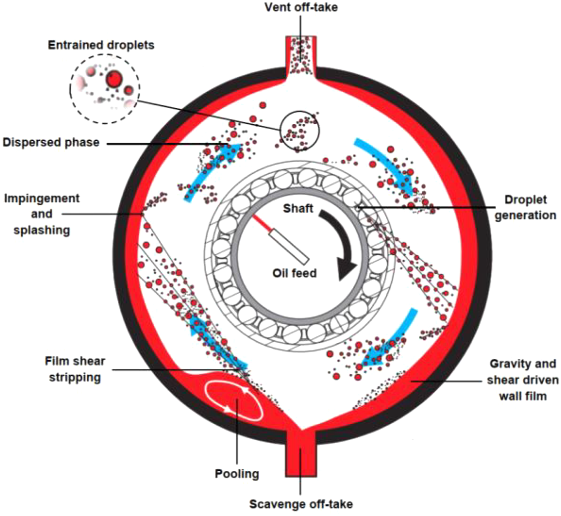
Simplified aeroengine bearing chamber flow physics, modified from Ref. 17.

The current industry best practice is to model turbulence quantities and account for turbulence effects using URANS based turbulence models. Considered as the state-of-the-art URANS approach, the shear stress transport (SST) k-ω turbulence model has been predominantly used within bearing chamber applications,^9–12 demonstrating the ability to capture the large vortical and swirling structures which dominate the flow. However, previous bearing chamber computational investigations have also investigated capability for the k-ϵ model^13,14 and its re-normalisation group (RNG) variant.¹⁰ In addition, several studies have been performed using the Reynolds stress model (RSM).^5,15,16 In the literature, whilst there have been a wide range of URANS turbulence modelling applications, currently there is no systematic data available which benchmarks the performance of these different turbulence modelling approaches available and their capability to capture the secondary airflow field.

Taylor–Couette studies

To date, there are very few combined CFD and experimental studies of rotating Taylor–Couette flow; in particular, investigations into the effect of the turbulence closure model selection on the predictions of Taylor–Couette systems are scarce. In recent years, the application of direct numerical simulation (DNS) to rotating Taylor–Couette flow has been the focus of many numerical studies for Reynolds numbers as high as 300,000.¹⁷ However, DNS is very computationally expensive and is not currently viable for industrially relevant geometries, highlighting the need for a modelling approach that is industrially applicable to rotating Taylor–Couette flows.

Wild et al.¹⁸ performed axisymmetric CFD simulations on narrow gap geometries, using the k-ϵ and RSM turbulence models. Comparison with experimental results showed that both the standard and RNG k-ϵ models over predicted results by at least 10%; whilst the RSM was found to perform poorly, over-predicting results by as much as 40%. More recently, Adebayo and Rona^19,20 investigated the velocity and pressure distributions for wide-gap Taylor–Couette flows using the realisable k-ϵ turbulence model. Within the weakly turbulent Taylor vortex flow regime, comparison of axial and radial velocity profiles against PIV data showed good agreement, with results inside the uncertainty band.

Batten et al.²¹ extended the work of Wild et al.¹⁸ with the use of the low Reynolds number k-ω turbulence model, over a range of axisymmetric geometries. For the narrow gap cases, $η = 0.941$ and 0.985, comparison to experimental data showed that the numerical simulations over-predicted velocities by approximately 20%, and for the wide-gap case, results were unreliable due to numerical problems resulting in differences of up to 40%.

Wang²² compared CFD data obtained from axisymmetric steady-state simulations with PIV experimental data up to the turbulent Taylor vortex flow regime. Due to the strong dependence of the Taylor cells on start-up conditions, as demonstrated by both Coles²³ and Koschmieder,²⁴ Wang defined a start-up protocol for their geometry, $η = 0.733$ , to ensure that a constant number of 14 Taylor vortex pairs formed over all of the rotation rates studied. Wang investigated a number of different turbulence models with various wall function approaches. Over the range of Taylor numbers investigated, comparison of velocity profiles showed that the RSM produced the closest trends to the experimental data but over predicted the maximum radial velocities by as much as 40%. Comparison of Reynolds stress contours also showed poor agreement.

The results of Wang²² are consistent with the numerical study performed by Poncet et al.,²⁵ who considered turbulent Taylor–Couette flow for a wide-gap geometry. The authors investigated a range of modelling techniques, such as the URANS RSM model, large eddy simulation (LES) techniques, including an SST k-ω SAS approach, and DNS. Out of the models investigated, the SST k-ω SAS model performed the worst, failing to predict the mean tangential velocity with a large overestimation compared to the experimental data. Surprisingly, all of the numerical approaches undertaken failed to reproduce the experimental mean tangential velocity and angular momentum profiles. Both the RSM and DNS provided the closest agreement to the experimental data, although failed to predict the shear stress components.

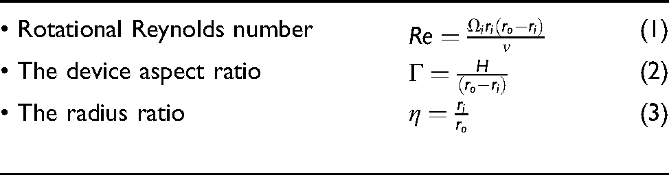
Experimentally, Coles²³ and Koschmieder²⁴ both demonstrate the significance of the device aspect ratio on the Taylor–Couette flow, including the number of vortices formed and the vortex axial wavelength, highlighting the influence of both the column length and the gap sizing. However, within bearing chamber applications, due to both the constrained axial length and gap size of the geometry, the space only permits a single vortex pair to form, as demonstrated by Gorse et al.³ As such, this parameter space is not explored within the Taylor–Couette flow investigations carried out in this work. It is also important to consider that many experimental and numerical studies of Taylor–Couette flow consider very long column lengths, such that when measurements are taken at the cylinder mid-gap, end effects become negligible. As such, the study on short aspect ratio Taylor–Couette devices is limited and the application within the turbulent Taylor vortex regime is even more scarce. This becomes important considering that aeroengine bearing chambers are essentially short aspect ratio systems. Burin et al.²⁶ experimentally investigated a short aspect ratio device, $Γ \sim 2$ with a high wall curvature, $η = 0.35$ for Reynolds numbers up to 400,000. For the range of Reynolds numbers investigated, the flow was highly turbulent, and visualisation showed a clear lack of vortex structure. Burin et al.²⁶ reported that due to the strongly unstable nature of the flow, the end wall effects had little effect on the fluid interior and therefore little influence on both the torque and velocity data.

From the literature reviewed, there have been limited applications of URANS turbulence modelling to Taylor–Couette flows; the literature points to the possibility that the RSM may be an adequate choice, although the results are still inconclusive. A limitation of most two-equation models is that the individual Reynolds stresses are not calculated and the three principal components ( $\bar{u^{'} u^{'}}$ , $\bar{v^{'} v^{'}}$ and $\bar{w^{'} w^{'}}$ ) are assumed equal: as such the turbulence is isotropic. The potential benefit of the RSM may be as a result of the ability to capture anisotropy due to resolving the individual stress components in the respective directions. It is also clear that the geometry and start-up conditions play a significant role in determining the final state achieved for Taylor–Couette flow and this needs to be carefully considered when validating CFD models.

Objectives

In general, for bearing chamber simulations, to date, whilst there have been a wide range of URANS turbulence modelling applications, currently there is no justification as to which is the most suitable URANS turbulence modelling approach. Furthermore, it is not well understood how geometrical and operational parameters influence turbulence within these systems. In an effort to better understand the complex bearing chamber environment, the geometry is first simplified to a Taylor–Couette domain. Within this configuration, a greater understanding of the turbulence modelling approach and the sensitivity to start-up conditions can be ascertained. Subsequently, this modelling capability will be extended to a bearing chamber geometry, in order to improve understanding surrounding the turbulence modelling approach and establish a solid foundation for future aeroengine bearing chamber investigations.

An objective of the current work is to, therefore, first perform a numerical comparison of both axisymmetric and three-dimensional URANS turbulence modelling approaches for a Taylor–Couette system. Due to considerable uncertainty within the literature, an objective of the work is to provide a best practical approach for the more advanced URANS turbulence models available. Furthermore, the sensitivity of results to the start-up conditions is of specific focus. The Taylor–Couette geometry under investigation corresponds to the configuration employed by Wang.²² Experimental measurements from the particle image velocimetry (PIV) data of Wang²² and the hot-wire results of Smith and Townsend²⁷ are used for comparison. Following this, the bearing chamber geometry of Gorse et al.³ is investigated and results are compared to the corresponding single-phase 3D laser Doppler anemometry (LDA) measurements presented by Gorse et al.³

Taylor–Couette investigations

Within Taylor–Couette flow, considering only rotation of the inner cylinder, the Taylor–Couette system depends predominantly on three main parameters:

• Rotational Reynolds number	$Re = \frac{Ω_{i} r_{i} (r_{o} - r_{i})}{ν}$	(1)
• The device aspect ratio	$Γ = \frac{H}{(r_{o} - r_{i})}$	(2)
• The radius ratio	$η = \frac{r_{i}}{r_{o}}$	(3)

Where $Ω_{i}$ is the rotational speed of the inner cylinder in rad/s, $r_{i}$ and $r_{o}$ are the inner and outer cylinder radii, respectively, $H$ is the height of the chamber and $ν$ is the kinematic viscosity of the fluid between the cylinders.

The geometry, shown in Figure 2, represents the computational domain based on the experimental apparatus used by Wang²² and consists of two concentric cylinders with inner and outer radii of 0.0349 and 0.0476 m, respectively. The length of the cylinders is 0.432 m, such that the aspect ratio of the geometry is 34, based on the gap size, 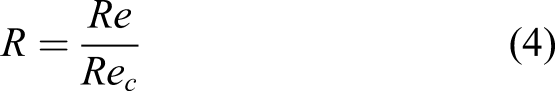$r_{o} - r_{i}$ , of 0.0127 m. The geometry results in a radius ratio $η$ of 0.733 resulting in a critical Reynolds number of $R e_{c} = 83.6$ . The critical Reynolds number defines the rotational Reynolds number for which the onset of Taylor vortices occurs; and here, its value is found through numerical interpolation of the linear theory presented by Donnelly et al.²⁸ It is also useful to define a Reynolds number ratio, which is the ratio of the rotational Reynolds number to the critical Reynolds number

R = \frac{R e}{R e_{c}}

(4)

Figure 2.

Computational domain and boundary conditions of Taylor–Couette geometry under investigation.

Wang²² focuses on only inner cylinder rotation. Through a specific start-up procedure, Wang²² ensures a fixed number of 14 Taylor vortex pairs formed at each rotation rate investigated. This was achieved through accelerating the inner cylinder from rest to a speed of 17.27 rad/s, at a constant angular acceleration of 0.0314 rad/s², and then maintaining this speed until 14 stable Taylor vortex pairs form, excluding the end cells. Subsequently, the inner cylinder is then either accelerated or decelerated at a constant rate of 0.314 and 0.126 rad/s² respectively, until the final desired state is reached. Wang²² maintained this final angular velocity for a short period before collecting PIV data. The measurements described were made over flow Reynolds numbers from 335 to 18,392, corresponding to Reynolds number ratios of 4–220; this covers the laminar Taylor vortex flow regime up to the weakly turbulent Taylor vortex flow regime. The fluid used by Wang²² has a density of 1055 kg/m³ and a dynamic viscosity of 1.097 × 10⁻⁰³ kg/ms.

Numerical methods

The finite volume incompressible solver, ANSYS Fluent 17.1, was used for all numerical calculations presented. The Semi Implicit Method for Pressure Linked Equations (SIMPLE) was chosen within the pressure-based solver, for which the PREssure STaggering Option (PRESTO) discretisation scheme was chosen due to the nature of the problem, based on the Fluent recommendations for high-speed rotating flows.²⁹ The solver was implemented with double precision and for time discretisation, a bounded second order implicit temporal discretisation scheme²⁹ was chosen to improve the accuracy and stability of the solution. All residuals were monitored and converged down to a minimum of 10⁻⁶.

Unsteady Reynolds-averaged Navier–Stokes turbulence modelling

Wang²² concluded that the RSM with standard wall functions was the most suited to model the flow field. Whilst it was found that for low rotation rates, the RSM predicted the mean velocity field with a reasonable degree of accuracy, at higher shaft speeds, there were large discrepancies. The computational results of Wang²² suggest that depending on the rotation rate, a number of different turbulence models are satisfactory to model the flow field, with the RSM giving the best agreement. However, at higher shaft speeds, for example, at R = 220, maximum radial velocities were over predicted by as much as 40%. In addition to this, Wang²² provides very limited details of the numerical investigation and based on the literature surveyed, there is inconclusive evidence as to which turbulence model yields the most satisfactory results. Hence, for this paper, a study into advanced turbulence models is conducted.

Several of the advanced URANS turbulence models available within ANSYS Fluent are investigated, to assess their suitability for Taylor–Couette flows, as well as more conventional models for comparison. These include the standard, realisable and RNG k-ϵ turbulence models; the standard, baseline (BSL) and SST k-ω turbulence models and the linear/quadratic and stress-omega/BSL Reynolds stress models. A more detailed analysis of the governing equations for each of the turbulence models presented can be found within the ANSYS theory guide²⁹ as well as the work of Versteeg and Malalasekera.³⁰

The k-ϵ model is regarded as the simplest of the two-equation models, it is a semi-empirical model based on the equations for the transport of turbulence kinetic energy (k) and its dissipation rate (ϵ). However, the RNG k-ϵ and the realisable k-ϵ model have shown to have an improved accuracy over the standard k-ϵ model without a significant increase in computational cost, especially for flow features involving strong streamline curvature, vortices and rotation.²⁹ The re-normalisation group (RNG) model includes the effect of swirl on turbulence and the accuracy for rapidly strained flows is improved through the addition of an extra term in the ϵ equation. The realisable k-ϵ turbulence model includes a modified transport equation for the dissipation rate (ϵ) and the turbulent viscosity has an improved formulation that varies the C_μ coefficient.

Two additional variants of the k-ω model exist, the baseline (BSL) k-ω model and the SST k-ω model. The standard k-ω model can exhibit a strong sensitivity to freestream conditions and as such the BSL k-ω model was developed, which blends the k-ω model in the near-wall region with the k-ϵ model in the freestream. The SST k-ω model includes the improvements of the BSL k-ω model; however, it also accounts for the transport of the turbulence shear stress. This results in a more robust formulation than the standard and BSL k-ω models, that is accurate and reliable for a wider class of problems.²⁹

The Reynolds stress model (RSM) solves a transport equation for each of the Reynolds stresses, in addition to an equation for the dissipation rate. This has the advantage of being inherently anisotropic and therefore is more complex and computationally expensive compared to the k-ε and k-ω models. Within Fluent, the default RSM is based on the ϵ-equation and uses either a linear or quadratic model for the pressure–strain term. The ω variants of the RSM both use a linear model for the pressure–strain term and however solve the scale equation differently. The stress-omega model derives from the ω-equation, whereas the stress-BSL model solves the baseline (BSL) k-ω scale equation, consequently removing the freestream sensitivity found with the stress-omega model. Both the ω-equation based variants are advantageous for modelling flows over curved surfaces and those involving swirling flows.²⁹

For all ϵ-equation based turbulence modelling, the enhanced wall treatment (EWT) approach is used. The EWT is an alternative near-wall modelling method that combines a two-layer approach suitable for finer meshes $(y^{+} < 1)$ with an enhanced wall function approach applicable for coarser meshes. The domain is divided into either a viscosity-affected region or a fully turbulent region. Within the fully turbulent region, the corresponding RSM or k-ϵ turbulence models are employed. However, within the near-wall viscosity-affected region, a low Reynolds number one-equation k-ϵ model²⁹ is employed. To achieve this, the enhanced wall treatment subsequently uses a blending function, modified depending on the wall distance between these two layers.

Axisymmetric modelling

The experimental apparatus of Wang²² was modelled initially as an axisymmetric case within Fluent using a structured grid, based on the suggestions from the literature reviewed. The computational domain is enclosed within the stationary outer cylinder and end walls while the inner cylinder rotates; at the walls, a no-slip condition is applied. The CFD domain represents a 2D slice of the Taylor–Couette experimental geometry, which greatly reduces the computational cost. It is possible to reduce the axisymmetric computational expense even further by simulating only one Taylor vortex pair through applying either periodic or symmetry boundary conditions at either end. Wang²² adopted a different approach whereby one quarter of the domain was modelled, incorporating one end wall and a symmetry boundary, resulting in the formation of only 3.5 vortex pairs. However, as the Reynolds number was increased further, the number of vortex pairs still varied such that Wang²² had to optimise the axial length for each rotational speed investigated. In this study, initial simulations showed that, whilst the domain maintains central symmetry, a $H / 2$ domain with a symmetric condition cannot be used. Firstly, imposing a symmetric boundary at $H / 2$ is not valid if the symmetry condition cuts a single Taylor vortex in half. Secondly, with the steady acceleration procedure, the shaft is accelerated to 17.27 rad/s, after which the speed is maintained until 14 stable Taylor vortex pairs form. Typically, more than 14 Taylor vortex pairs first form and, after maintaining this speed, this number converges down to a fixed state of 14 Taylor vortex pairs. The use of a symmetry condition fixes the position of Taylor vortices, which does not allow the vortices to reduce in number and converge down to 14 pairs. It is clear that to eliminate these uncertainties it is necessary to model the full length of the computational domain, in order to incorporate end effects and achieve the desired final state of 14 Taylor vortex pairs.

In the present study, Ansys ICEM software was used to generate all of the grids. For simplicity, initial computational modelling is two-dimensional where an axisymmetric grid is used with predictions for the swirl/circumferential velocity included. Table 1 summarises the grid configurations explored in the mesh sensitivity study.

Table 1.

Axisymmetric grids for mesh independence study.

Mesh	Grid (radial × axial)	Number of cells	$y^{+}$ values
A	20 × 680	13,600	5 < y⁺ 15
B	40 × 1050	42,000	1 < y⁺ 10
C	40 × 1050	42,000	$y^{+} \leq$ 1
D	75 × 2100	157,500	$y^{+} \leq$ 1
E	110 × 3150	346,500	$y^{+} \leq$ 1

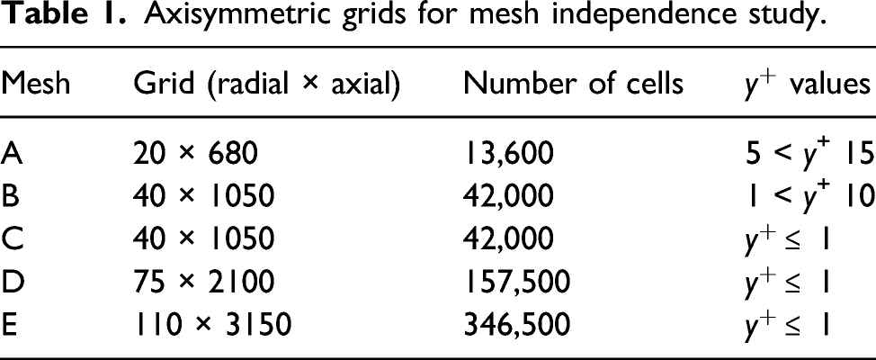
Whilst a fully mesh independent solution was not reached for all simulations, it was judged that sufficiently low mesh dependence was achieved for the purpose of this study. Table 2 presents the computed non-dimensionalised shaft torque, $G = M / (2 π ρ ν^{2} H)$ , and gauge static pressure at $H / 2$ on the outer cylinder wall, which are used to assess mesh independence for both the standard k-ε and k-ω turbulence models in order to establish a baseline mesh. These variables are monitored to give an understanding of mesh dependency on both a global and local scale within the flow field. The mesh dependency tests showed that with the k-ω turbulence model, it was slightly more difficult to reach a mesh independent solution when compared to the k-ε turbulence model, requiring a finer level of grid refinement.

Table 2.

Axisymmetric mesh independence study results for the standard k-ε and standard k-ω turbulence models.

	Standard k-ε		Standard k-ω
Mesh	G (×10⁵)	Static pressure (Pa)	G (×10⁵)	Static pressure (Pa)
A	4.930	29.19	6.219	38.19
B	4.065	27.24	4.997	38.21
C	3.892	26.88	4.926	40.26
D	3.893	26.95	4.901	40.70
E	3.893	26.96	4.861	41.64

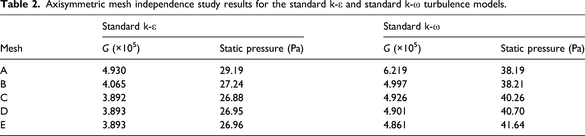
Overall, across both turbulence models, there was a percentage difference of $< 1 %$ between Meshes D and E, for both the respective torque and pressure values in Table 2. As such, Mesh D was chosen for all further axisymmetric simulations with a final grid of 157,500 cells, with $y^{+} \leq 1$ .

In the following sections, axisymmetric CFD results are compared to the radial velocity profiles of Wang²² and for all simulations, results were time averaged over a duration of six inner cylinder rotations.

Start-up procedure

As demonstrated both by Coles²³ and Koschmieder,²⁴ the final state of Taylor–Couette flow exhibits a strong dependence on starting conditions. In order to reproduce the experimental data of Wang,²² it was found to be necessary to compile a user defined function (UDF) to exhibit the same start-up procedures used experimentally. The sensitivity of the solution to start-up conditions was investigated computationally through comparing Taylor vortex axial lengths with those observed experimentally by Wang.²² The developed start-up UDF was compiled and linked within Fluent for both the k-ϵ and k-ω models over the range of rotational Reynolds number ratios considered experimentally by Wang.²² This was to assess the influence of sudden start accelerations of the inner cylinder compared to the steady acceleration procedure outlined by Wang,²² as described in the section Taylor–Couette Investigations. A typical acceleration procedure obtained through the UDF is described below; the process can be split into four stages:

• Stage 1	–	Acceleration at 3.14 rad/s² to Ω_i = 17.27 rad/s
• Stage 2	–	Maintain angular velocity till 14 Taylor vortex pairs form and stabilise
• Stage 3	–	Accelerate at 3.14 rad/s² or decelerate at 0.126 rad/s² to the final desired speed
• Stage 4	–	Maintain angular velocity till solution stabilises

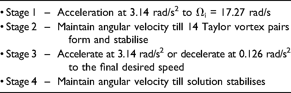
Figure 3 presents the velocity vector field for a typical Taylor vortex pair formed after the steady acceleration procedure as described above; here, the rotation Reynolds number ratio is R = 220.

Figure 3.

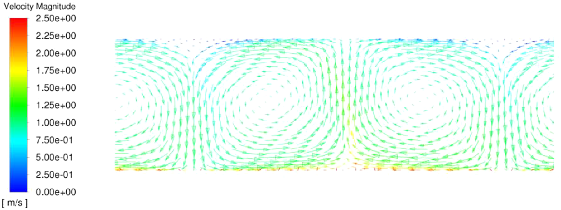
Velocity vector field for a Taylor vortex pair at R = 220 after the steady acceleration procedure.

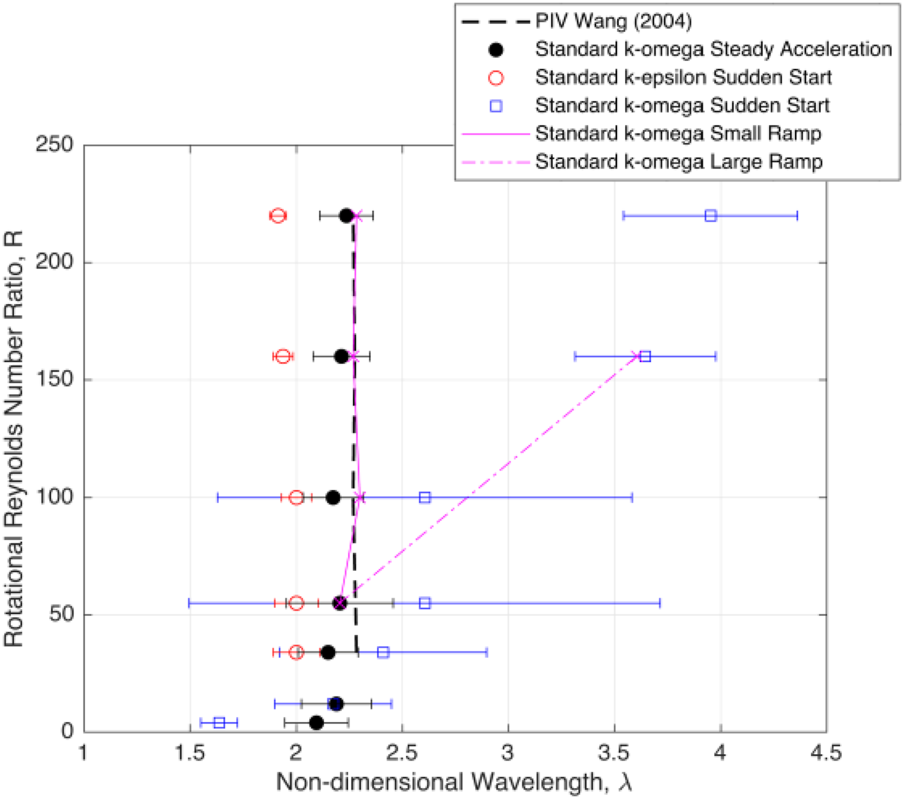
Figure 4 shows a comparison of the different non-dimensional wavelengths, λ, obtained for the rotational Reynolds number ratios ranging from 4 to 220. The wavelength is defined as the axial extent of one Taylor vortex pair and this is non-dimensionalised by the gap size, $r_{o} - r_{i}$ . The black dashed line shows the wavelength extrapolated from the experimental data of Wang,²² for which the wavelength varied from 2.268 to 2.284 resulting in a total number of 14 Taylor vortex pairs.

Figure 4.

Axial wavelengths for sudden start and steady acceleration procedures.

The average wavelength recorded for sudden start cases is displayed, with the red circles representing the standard k-ϵ turbulence model and the k-ω turbulence model shown with blue squares. For each data set, the error bars represent the standard deviation in the axial wavelength. Immediately, it is clear that there is a significant difference in wavelength obtained based on the turbulence model used. In general, the k-ω turbulence model produced Taylor vortices with a larger average wavelength than the PIV data, meaning the number of Taylor vortex pairs was less than the desired value of 14, for example at $R = 55$ , the number of Taylor vortex pairs was 12 and this decreased to 7 pairs at $R = 220$ . In contrast, the k-ϵ turbulence model produced a uniform but shorter wavelength over all of the rotational Reynolds number ratios, resulting in 15 Taylor vortex pairs.

The simulations performed for the steady acceleration procedure, depicted by the solid black circles, were carried out for both the k-ϵ and k-ω models; between the two models, there was a negligible difference in results; hence, only the results from the standard k-ω model are shown in Figure 4. At all of the rotation rates investigated, 14 Taylor vortex pairs were formed following the steady acceleration period; furthermore, the PIV data of Wang²² falls within the standard deviations for all cases, resulting in a percentage difference in average wavelengths of 1.4 to 5.9%, with the greatest difference occurring at the slowest speed at $R = 34$ . Interestingly, as the rotational Reynolds number ratio is increased, the difference in average wavelengths between the PIV and steady acceleration data decreases and at $R = 220$ , the percentage difference is only 1.4%. The results of the steady acceleration procedure are in agreement with the experimental data of Koschmieder²⁴ produced for the wide-gap apparatus.

Figure 4 also shows a comparison of the non-dimensional axial wavelength following either a small or large step in the rotation rate of the inner cylinder once the $14$ Taylor vortex pairs have first formed and stabilised at $R = 55$ . For the small step in rotation rate (solid line), the rotational Reynolds number was increased in steps from $R = 55 \to 100 \to 160 \to 220$ , whereas the large step in rotation rate (dashed-dot line) was increased in a step from $R = 55 \to 160$ . For a large step in the inner cylinder speed, the average wavelength obtained was 3.606, which is much larger than that obtained experimentally, resulting in the formation of only 10 Taylor vortex pairs and, therefore, closely resembling the result obtained after a sudden start to $R = 160$ . In contrast, for a small step in the inner cylinder speed, there is much less variation in the wavelength obtained compared to the steady acceleration procedure. Furthermore, following a small step, the axial wavelength approaches the experimental results of Wang²² resulting in a percentage difference of wavelengths ranging from 0.5 to 1.4%. These results support the findings of Koschmieder,²⁴ showing that once the Taylor vortex pairs are established, they are very stable to small steps in the rotational Reynolds number ratio, as opposed to a large step.

Overall, these results show that by using an appropriate start-up approach it is possible to obtain good agreement on the number of Taylor cells compared to the experimental data of both Wang²² and Koschmieder²⁴ for wide-gap geometries. This gives confidence in the steady acceleration procedure employed computationally, showing that it is possible to achieve the same time-averaged number of Taylor vortices reported in the experiment in the turbulent Taylor vortex flow regime.

Unsteady Reynolds-averaged Navier–Stokes turbulence modelling

The turbulence models described in the Start-up Procedure section are compared against the PIV non-dimensional velocity profiles of Wang²² including both maximum and minimum radial velocities. The aim of this study is to determine the most appropriate turbulence modelling strategy applicable to a rotating Taylor–Couette geometry.

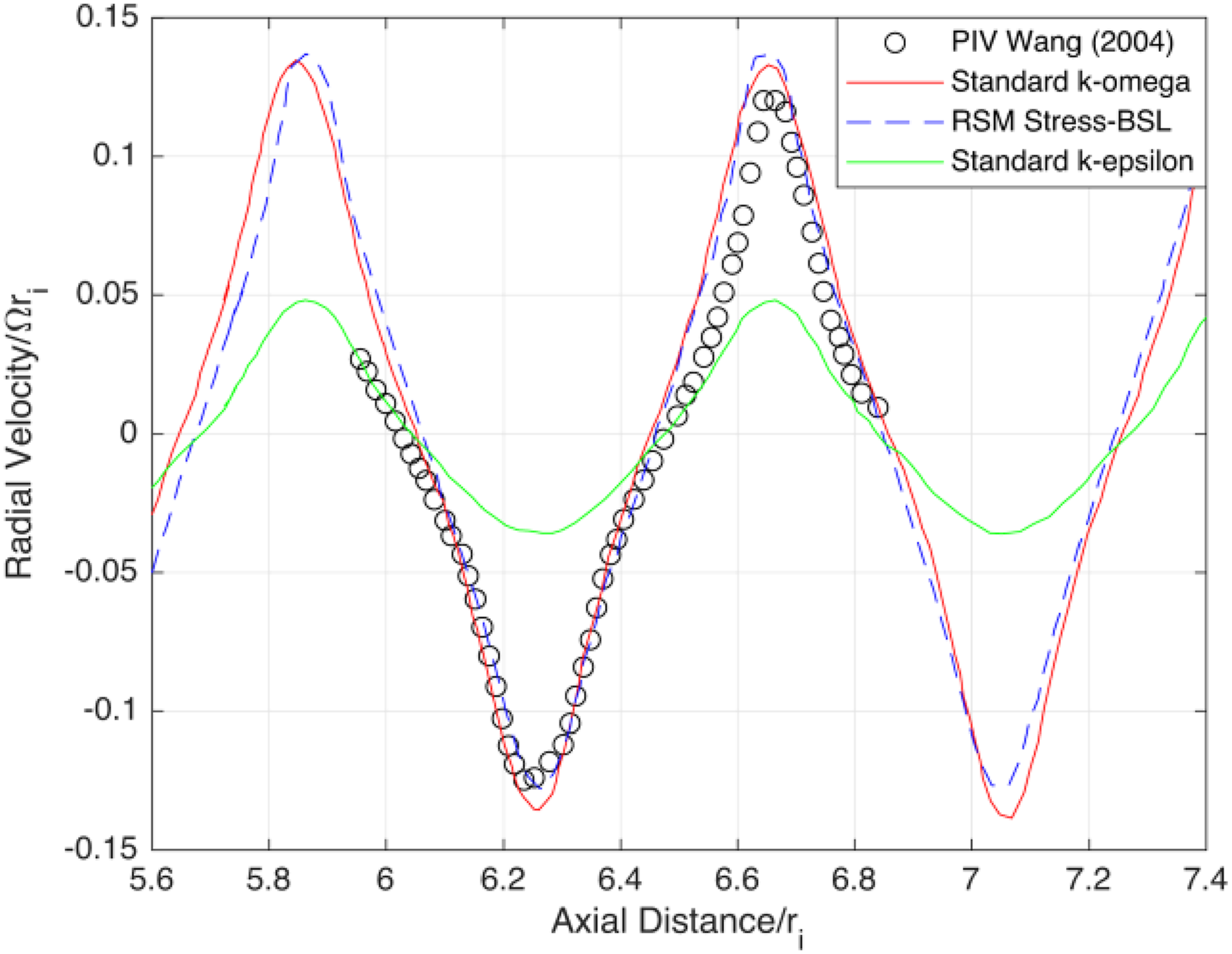
Firstly, the results from the turbulence models at $R = 100$ , are compared to the radial PIV velocity profiles of Wang,²² taken along an axial line at a height of one third of the gap width, positioned from the inner cylinder. Out of all of the turbulence models investigated, it was found that both the standard k-ω and RSM stress-BSL turbulence models gave the closest agreement. A sample of the results obtained is provided in Figure 5, showing a comparison of the non-dimensional radial velocity profile predicted by these two turbulence models, here the radial velocity is non-dimensionalised by the circumferential shaft velocity, $Ω r_{i}$ . For reference, within Figure 5, the results of the standard k-ϵ model are also shown.

Figure 5.

Comparison of non-dimensional radial velocity profiles at R = 3.94 cm and R = 100.

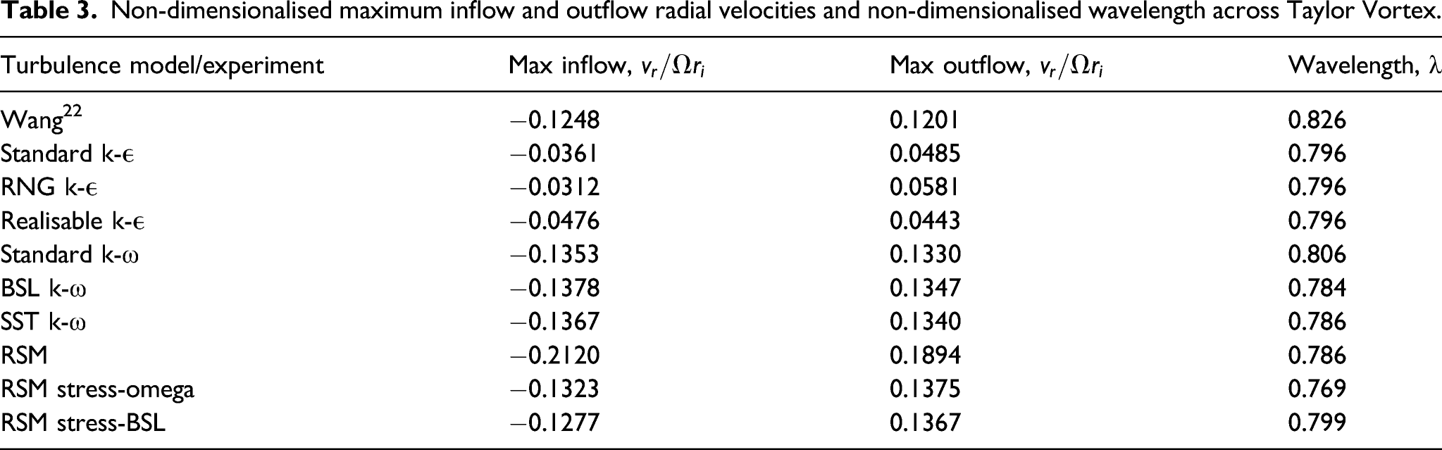
Furthermore, Table 3 provides the non-dimensionalised maximum Taylor vortex inflow (negative $v_{r}$ ) and outflow (positive $v_{r}$ ) radial velocities for each of the turbulence models and the experimental PIV measurements of Wang²² at $R = 100$ . A Taylor vortex inflow boundary occurs where fluid is convected radially inward between a pair of Taylor vortices; the opposite is true for the outflow Taylor vortex boundary. Table 4 highlights the corresponding percentage difference between the experimental results of Wang,²² and the numerical values predicted across all of the turbulence models investigated. Additionally, within Table 3, wavelength data is included and Table 4 gives the percentage difference between the average non-dimensional Taylor vortex wavelength predicted computationally versus that obtained experimentally.

Table 3.

Non-dimensionalised maximum inflow and outflow radial velocities and non-dimensionalised wavelength across Taylor Vortex.

Turbulence model/experiment	Max inflow, $v_{r} / Ω r_{i}$	Max outflow, $v_{r} / Ω r_{i}$	Wavelength, λ
Wang²²	−0.1248	0.1201	0.826
Standard k-ϵ	−0.0361	0.0485	0.796
RNG k-ϵ	−0.0312	0.0581	0.796
Realisable k-ϵ	−0.0476	0.0443	0.796
Standard k-ω	−0.1353	0.1330	0.806
BSL k-ω	−0.1378	0.1347	0.784
SST k-ω	−0.1367	0.1340	0.786
RSM	−0.2120	0.1894	0.786
RSM stress-omega	−0.1323	0.1375	0.769
RSM stress-BSL	−0.1277	0.1367	0.799

Table 4.

Percentage difference (%) in both non-dimensionalised average velocity and wavelength across Taylor vortex.

Turbulence model	Inflow, $v_{r} / Ω r_{i}$	Outflow, $v_{r} / Ω r_{i r}$	Wavelength, λ
Turbulence model	% difference	% difference	% difference
Standard k-ϵ	59.1	36.6	3.6
RNG k-ϵ	55.0	28.6	3.6
Realisable k-ϵ	61.9	40.1	3.6
Standard k-ω	8.4	10.8	2.4
BSL k-ω	10.4	12.2	5.1
SST k-ω	9.5	11.6	4.8
RSM	69.9	57.8	4.8
RSM stress-omega	6.0	14.5	6.9
RSM stress-BSL	2.3	13.9	3.3

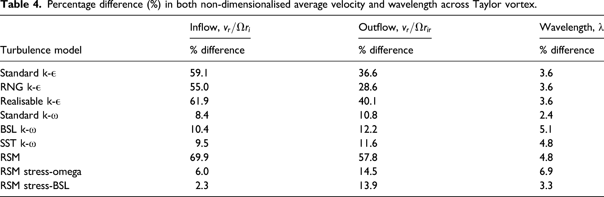
Results obtained for the standard, RNG and realisable k-ϵ turbulence models showed a significant deviation from the PIV measurements of Wang²² in terms of radial velocities. It should be noted that, when comparing the results of the ϵ-based turbulence models against each other, there was very little deviation in radial velocity profiles; whilst the models all predicted a similar profile, the peak values differed by as much as 60% from the experimental measurements, as shown in Table 4. This is also highlighted in Figure 5 for the standard k-ϵ turbulence model. Overall, from the investigation into ϵ-equation based turbulence modelling, it was clear that the none of the models investigated produced satisfactory results.

In contrast, the standard, BSL and SST k-ω turbulence models all produced a much closer agreement with the experimental data, however the standard k-ω turbulence model provided the most accurate results in terms of radial velocity profiles, evident from Table 4. Both the BSL and SST k-ω models produced reasonable agreements compared to the standard k-ω model, although as highlighted in Table 4, the axial wavelength of the Taylor vortex pairs was slightly worse, here, over-predicting by approximately 5%, resulting in smaller end cells.

An investigation into the RSM variants was also carried out. The standard RSM, which relies on the underlying assumptions associated with ϵ-equation modelling, was found to be inappropriate in predicting the flow field for both the radial velocity and mean velocity distribution across the gap, with results similar to those produced by the standard k-ϵ model, shown in Table 4. Interestingly, the quadratic-pressure strain model failed to produce any Taylor vortex structure over all of the rotational Reynolds number ratios investigated. However, the ω-based variants of the RSM showed significant improvements with the best results obtained using the RSM stress-BSL model, as opposed to the RSM stress-omega variant, which in relative comparison, over-predicted the axial wavelength, Table 4.

As the rotational Reynolds number ratio is increased, the differences between the computational and the experimental results of Wang²² start to become apparent. This is evident from Table 5 which summarises the percentage difference in the non-dimensional maximum inflow and outflow radial velocities, averaged over each of the 14 Taylor vortex pairs, for each rotational Reynolds number ratio investigated. At $R = 220$ , both the standard k-ω and the RSM stress-BSL turbulence models over predict the inflow and outflow Taylor vortex boundaries, resulting in differences as large as 70%. In general, as the rotational Reynolds number ratio is increased, the percentage difference rapidly increases for both turbulence models.

Table 5.

Percentage difference in non-dimensional radial velocities across Taylor vortex in/outflows.

R	PIV Wang²²		Standard k-ω		RSM stress-BSL
	Max inflow, $v_{r} / Ω r_{i}$	Max outflow $v_{r} / Ω r_{i}$	Inflow, $v_{r} / Ω r_{i}$	Outflow, $v_{r} / Ω r_{i}$	Inflow, $v_{r} / Ω r_{i}$	Outflow, $v_{r} / Ω r_{i}$
	Max inflow, $v_{r} / Ω r_{i}$	Max outflow $v_{r} / Ω r_{i}$	% difference	% difference	% difference	% difference
34	−0.0649	0.0686	2.9	32.2	2.0	28.7
100	−0.1248	0.1201	8.4	10.8	2.3	13.9
160	−0.1656	0.1784	22.2	13.3	31.0	31.4
220	−0.1807	0.1963	70.1	54.3	55.0	71.1

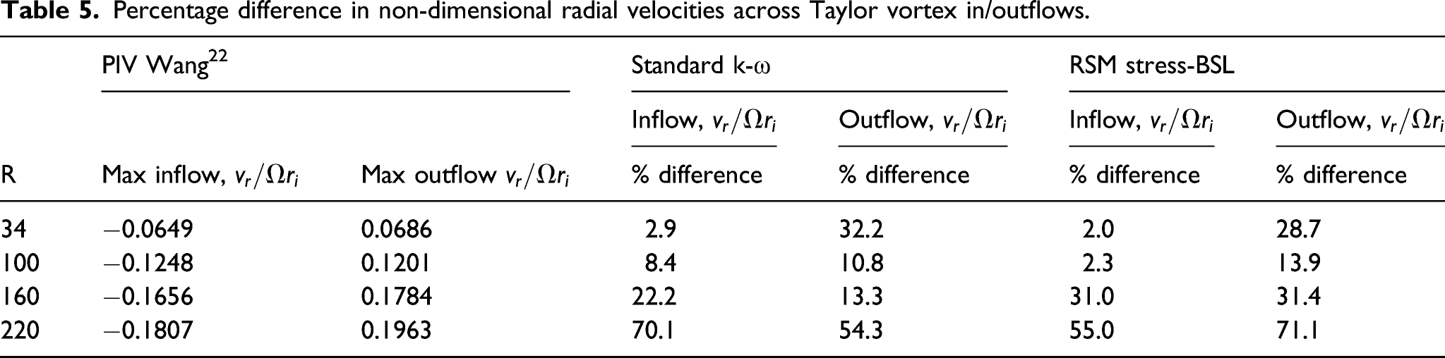
In conclusion, the axisymmetric URANS turbulence modelling study has shown the standard k-ω model provides satisfactory results and is able to capture the key characteristics of the flow, although at large Reynolds number ratios, this agreement is poor in terms peak radial velocities. The RSM stress-BSL model provides comparable results to the standard k-ω turbulence model, although at a significant increase in computational cost. However, as the rotational Reynolds number is increased, poor agreement is found for both models suggesting that as turbulence increases, an axisymmetric approach is unsuitable. It is suspected that the axisymmetric modelling methodology starts to break-down, as a result of not being able to predict the three-dimensional structures typically found within turbulent Taylor––Couette flows, such as Görtler vortices^27,31 present within the boundary layers; as opposed to the lack of capability within the turbulence models. As such, subsequent modelling will apply the axisymmetric modelling methodology developed to a three-dimensional domain for both the standard k-ω and RSM stress-BSL turbulence models.

Three-dimensional modelling

Following the results of the axisymmetric URANS study, the start-up procedures and turbulence models used were applied to a three-dimensional model. As such, the operating conditions and fluid properties were kept the same. From the axisymmetric simulations, it has been observed that there are a number of three-dimensional effects that may be suppressed by axisymmetric modelling. As such, it is still unclear whether the axisymmetric turbulence modelling approach is still applicable when applied to three-dimensional modelling.

For 3D Taylor–Couette simulations, Brauckmann and Eckhardt³² showed simulation complexity could be heavily reduced through applying both axial and rotational periodicity. Brauckmann and Eckhardt³² demonstrated that in general the modelled geometry could be heavily simplified through simulating only one Taylor vortex pair with a rotational symmetry of order six. However, more recently, the DNS study carried out by Ostilla-Mónico et al.³³ suggests that applying both axial and rotational periodicity imposes constraints on the flow field, which, despite generating accurate velocity data, can affect the overall bulk statistics. The results from Ostilla-Mónico et al.³³ did not reach an independent solution and recommendations are made to determine the extent to which the domain can be limited to produce accurate velocity and pressure fluctuation statistics in addition to higher order moments. The results from this current work suggest that for accurate velocity and turbulence data, the whole domain may need to be modelled. This will be investigated by carrying out a study into applying rotational periodicity to the three-dimensional domain and comparing to the available experimental data.

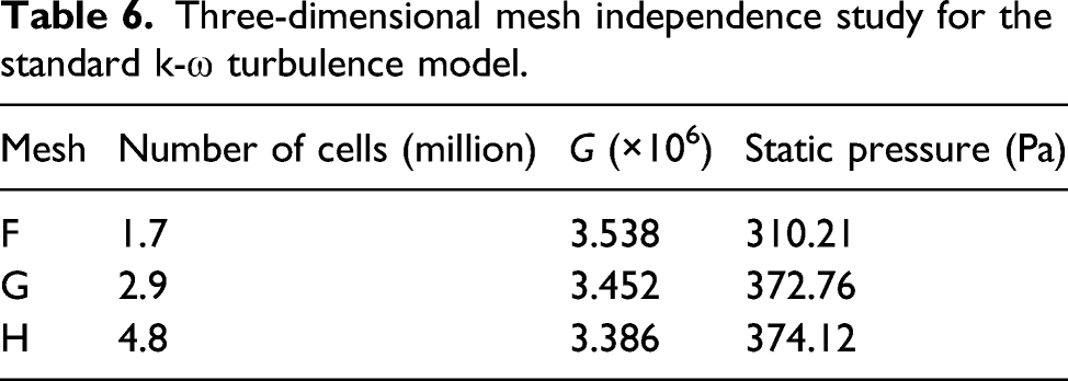
Similar to the axisymmetric URANS study, a three-dimensional mesh independence study was first carried out. An equivalent numerical method and solution procedure was retained. Whilst Mesh D was chosen to be appropriate for the axisymmetric modelling, the coarser mesh, Mesh C was chosen as a starting point for the three-dimensional modelling. To begin with, the radial and axial grid spacing of Mesh C was transformed through 360° about the axis of rotation, resulting in a mesh of 1.7 million cells. Through removing the axisymmetric assumption, it is deemed appropriate to start the three-dimensional meshing from a coarser grid and subsequently refine the mesh until a mesh independent solution is achieved. Although a fully mesh independent solution was not obtained, through monitoring torque values and static pressure on the outer cylinder wall, a relatively low mesh dependence was observed. A final mesh containing 4.8 million cells with a wall spacing of $y^{+} \leq 1$ and a growth ratio of 1.2 was deemed adequate; resulting in a percentage difference of less than 2% in computed torque values. This mesh is depicted in Figure 2, for which Table 6 presents the computed non-dimensionalised shaft torque, G, and static pressure at H/2 on the outer cylinder wall at $R = 220$ , which was used to assess mesh independence.

Table 6.

Three-dimensional mesh independence study for the standard k-ω turbulence model.

Mesh	Number of cells (million)	G (×10⁶)	Static pressure (Pa)
F	1.7	3.538	310.21
G	2.9	3.452	372.76
H	4.8	3.386	374.12

Start-up procedure

The results obtained from the axisymmetric investigation into the start-up procedure were also investigated for the three-dimensional configuration. It was observed that the outlined start-up procedure remained accurate for three-dimensional simulations and as such a new UDF was developed and linked within Fluent. This new UDF included the previous steady acceleration to $R = 55$ , which is the point at which 14 Taylor vortex pairs form and stabilise, after which the UDF was optimised to incorporate small steps in the inner cylinder speed. These steps varied the inner cylinder speed in steps from $R = 55 \to 110 \to 165 \to 220$ . At each step of the inner cylinder speed, in addition to verifying the 14 Taylor vortex pairs, several parameters were monitored for convergence including: the residuals, each velocity component, and the turbulent kinetic energy. Typically, after six revolutions of the inner cylinder the monitors had converged.

The purpose of modifying the UDF was to remove the substantial computational cost associated with slowly accelerating from $R = 55$ to $R = 220$ and therefore significantly reducing the computational runtime required for three-dimensional simulations. This resulted in reducing the computational cost of simulations by as much as 20 and 25% for the standard k-ω and RSM stress-BSL turbulence models, respectively.

Rotational periodicity study

In order to see if the computational cost associated with the three-dimensional simulations could be reduced further, a study into applying rotational periodicity was carried out. Brauckmann and Eckhardt³² suggest that a rotational periodicity of $60 °$ provides accurate results, however with a geometry of $η = 0.714$ Brauckmann and Eckhardt³² were also successful in applying a rotational periodicity of $40 °$ . As such, three new meshes were generated from the full three-dimensional mesh, resulting in the periodic segments of $45 °$ , $90 °$ and $180 °$ .

A sample of the results are shown in Figure 6, which includes the result obtained from the standard k-ω turbulence model for the $90 °$ and $180 °$ meshes since there was very little difference when compared to the RSM stress-BSL predications. Results are not shown for the simulations carried out using the $45 °$ mesh. At $45 °$ , once the rotational Reynolds number ratio of $R = 55$ was reached, the simulation converged to a fixed state of 17 Taylor vortex pairs for both turbulence models, even after maintaining this velocity for a prolonged period. As such, further investigations into the $45 °$ mesh were not carried out.

In addition to this, similar problems were also experienced with the $90 °$ mesh, and the simulations converged to and remained fixed at 15 Taylor vortex pairs over all of the rotational Reynolds numbers investigated. The same outcome was still reached even without the optimised start-up procedure. Whilst both turbulence models did not reach the desired 14 Taylor vortex pairs, a comparison was still made to the radial PIV velocity data of Wang.²² It should be noted that the results from the $180 °$ mesh did indeed result in the formation of 14 Taylor vortex pairs. From Figure 6, it is clear that both periodic segments over predict the inflow and outflow Taylor vortex boundaries significantly, similar to the results obtained from the two-dimensional axisymmetric modelling approach. Furthermore, a more linear transition across the inflow to outflow vortex boundary is observed for both the $90 °$ and $180 °$ cases.

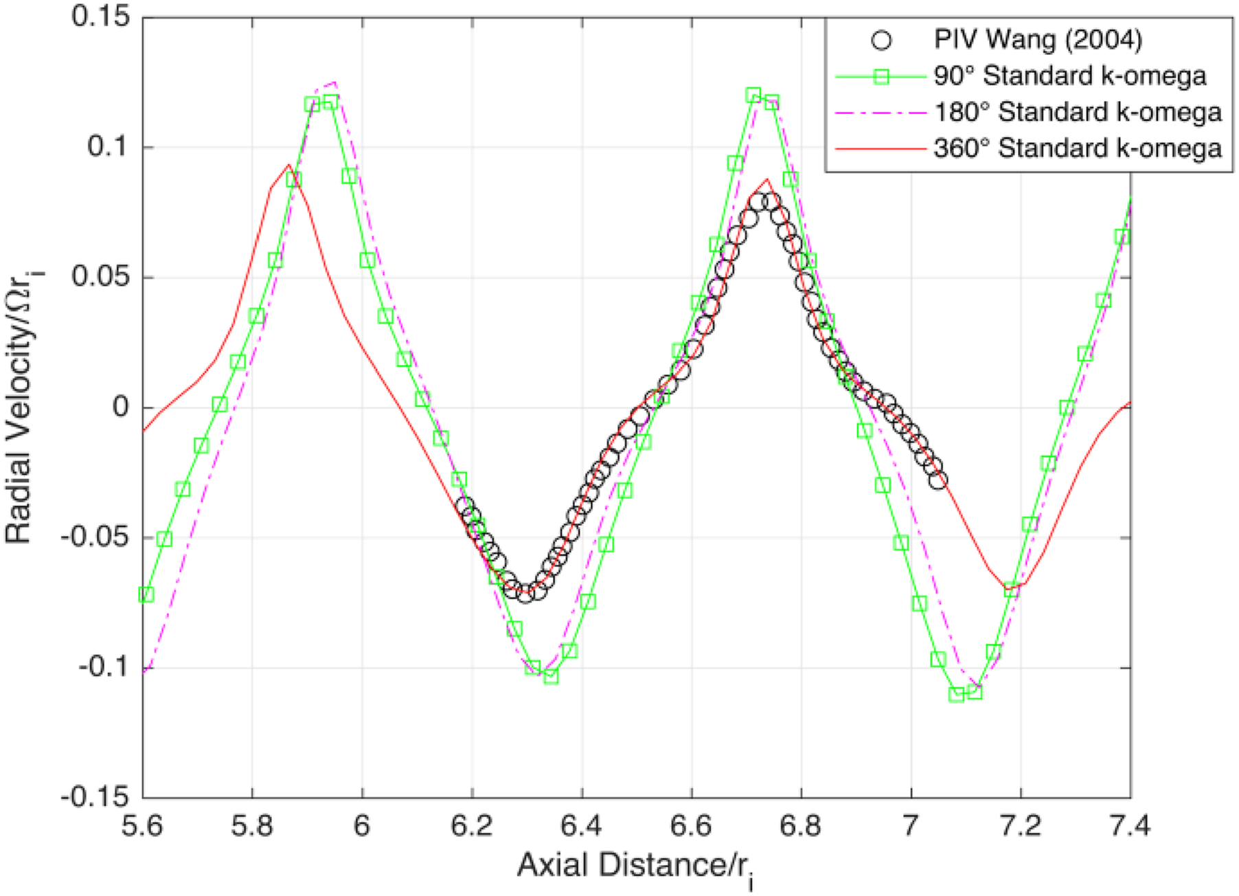
Analysis of the non-dimensional velocity magnitude profile across the annular gap with the hot-wire data of Smith and Townsend²⁷ at an equivalent gap spacing and a similar Reynolds number ratio of $R = 225$ is presented in Figure 7. The velocity magnitude profiles are averaged over the central Taylor vortex pair since within the experiments of Smith and Townsend,²⁷ a slow axial flow was induced to traverse the stationary Taylor vortices over the stationary hot-wire anemometers.

Figure 6.

Comparison of non-dimensional radial velocity profiles at a radius of 3.94 cm and R = 220 when varying the domain rotational periodicity.

Figure 7.

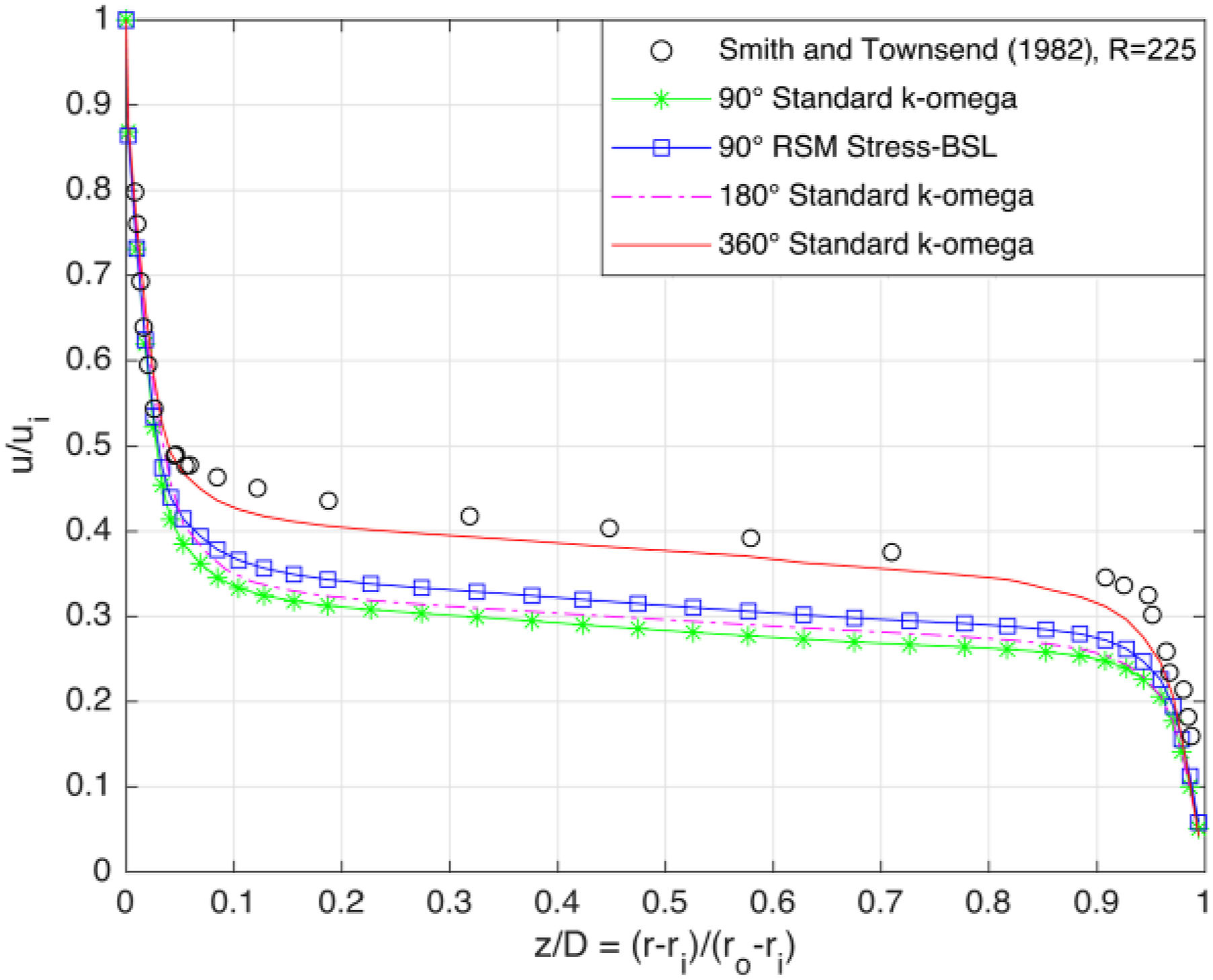
Non-dimensional velocity magnitude across annular gap at R = 220.

Within Figure 7, the results of both the $90 °$ and $180 °$ sectors for the standard k-ω turbulence model reveal that between the two cases whilst there is a negligible difference, the overall core velocity is significantly reduced. At the non-dimensional distance of 0.581, the non-dimensional velocity magnitude for both the standard k-ω predictions is approximately 0.277 compared to that reported by Smith and Townsend²⁷ of 0.390 $\pm$ 0.001 giving a percentage difference of almost 29%. Only a slight improvement in this core velocity is seen when switching from the standard k-ω to the RSM stress-BSL turbulence model. In Figure 7, for the RSM stress-BSL model, only the results from the $90 °$ segment are shown due to the negligible difference at $180 °$ . At the non-dimensional distance of 0.581 the non-dimensional velocity is 0.306 resulting in a percentage difference of 21.5%.

These results contrast with the findings from the DNS study of Brauckmann and Eckhardt³² relating to using rotational periodicity. For the current geometry with a URANS turbulence modelling approach, applying rotational periodicity is not feasible and results in a significantly reduced core velocity. This implies that for three-dimensional URANS turbulence modelling the full $360 °$ geometry must be implemented in order to not impose any constraints on the flow and thus accurately resolve the flow field. For the three-dimensional models, the use of symmetry in the axial direction was not investigated based on the conclusions drawn from the axisymmetric study.

Three-dimensional results

Within a fully developed turbulent flow, the turbulent structures and generating processes are inherently three-dimensional. Therefore, it is important to re-assess if the conclusions drawn from the URANS axisymmetric turbulence modelling study still remain valid. As such, a turbulence modelling study was again performed for the three-dimensional configuration.

Unlike the axisymmetric study, all of the ϵ-equation-based turbulence models severely over-predicted both radial and axial velocities, with maximum radial velocities over-predicted by as much as 85%. Figure 8 shows an example of the standard k-ϵ turbulence model compared against the PIV data of Wang.²² In contrast, good agreement was still found for the ω-equation turbulence models and the inferences on model effectiveness from the axisymmetric simulations remained valid. As such, for the three-dimensional simulations, the numerical modelling strategy outlined in the Axisymmetric Modelling section was carried forwards using both the standard k-ω and RSM stress-BSL turbulence models. For both turbulence models, results were again time averaged over a duration of six inner cylinder rotations.

Figure 8.

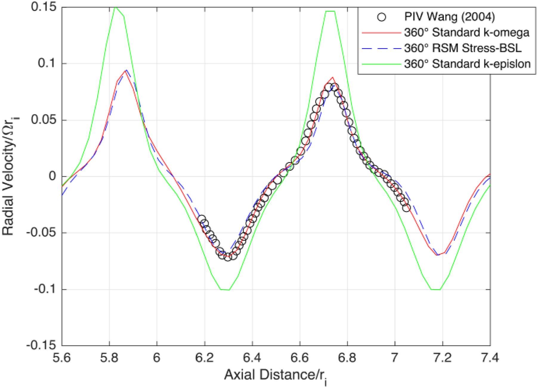
Comparison of non-dimensional radial velocity profiles at a radius of 3.94 cm and R = 220 for the full 360° domain.

The radial velocity profiles shown in Figure 8 illustrate that both the standard k-ω and RSM stress-BSL turbulence models provide excellent agreement with the PIV data of Wang²² at $R = 220$ , significantly improving on the two-dimensional axisymmetric results and the periodicity study. Taylor vortex boundaries are accurately represented with the percentage differences for both turbulence models much less than 1%. Upon closer inspection, the RSM stress-BSL turbulence model predicts the overall PIV radial profile to a slightly greater degree of accuracy.

Comparison of velocity magnitude profiles across the annular gap with the hot-wire data of Smith and Townsend,²⁷ shown in Figure 9, reveals that there is negligible difference between the two turbulence models. 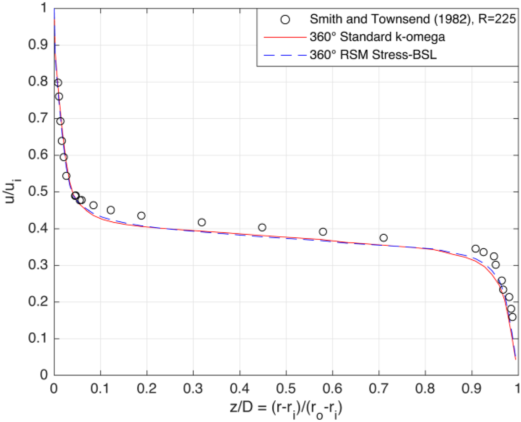Both turbulence models predict a slightly reduced non-dimensional core velocity of 0.371 at the non-dimensional distance of 0.581 which results in a percentage difference of less than 5% when compared to that of 0.390 $\pm$ 0.001 reported by Smith and Townsend.²⁷ This difference can most likely be attributed to the discrepancies in geometry and operational conditions between the two investigations.

Figure 9.

Non-dimensional velocity magnitude across annular gap at R = 220.

Bearing chamber investigations

Following the Taylor–Couette URANS turbulence modelling investigation, the methodology is extended to an aeroengine bearing chamber application. A study into the single-phase airflow is conducted with comparison to the experimental 3D Laser Doppler Anemometry (LDA) measurements performed by Gorse et al.³ on a high-speed bearing chamber test rig. The experimental configuration of Gorse et al.³ focuses purely on the influence of airflow within the chamber, highlighting the dependence of secondary airflow structures on both the rotational shaft speed and sealing airflow rates in the absence of oil. A cross-section of the front bearing chamber under investigation is shown in Figure 10. The chamber consists of a shaft throughout the length of the domain, with a diameter D = 128 mm. The resulting diameter and axial length of the bearing chamber are 1.73D and 0.34D, respectively. In relation to the Taylor–Couette analogy, this results in a radius ratio, η = 0.577, and a device aspect ratio, Γ = 0.47, therefore, a small aspect ratio, wide-gap system.

Figure 10.

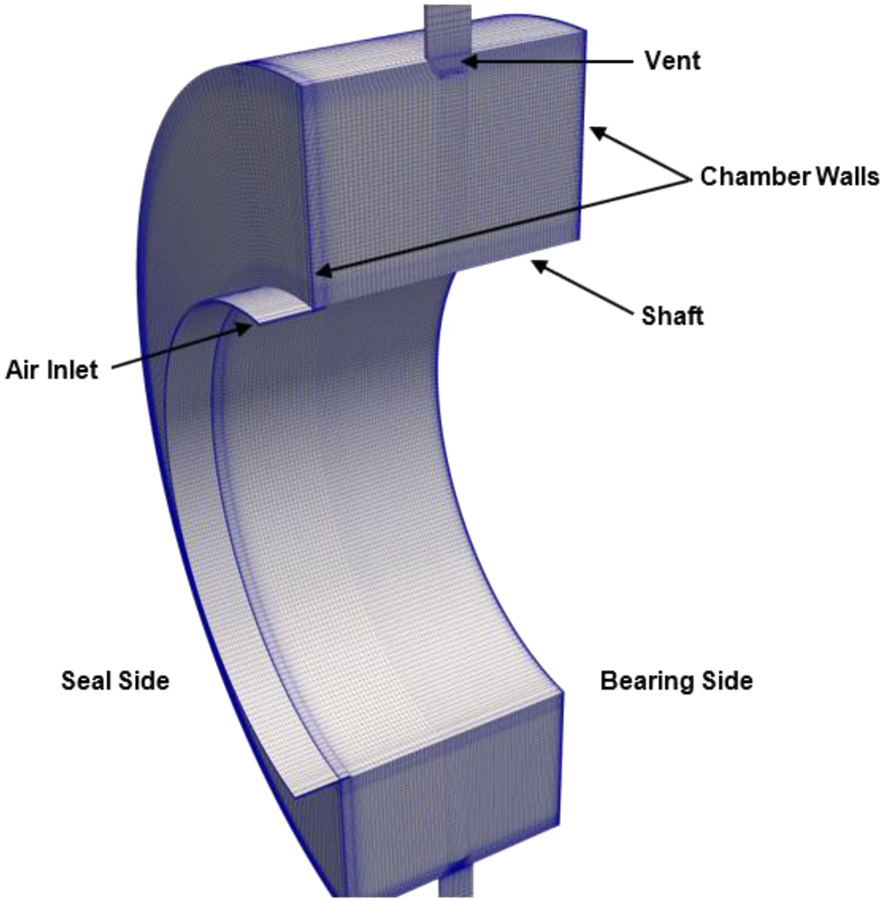
Computational cross-section of the Gorse et al. bearing chamber.

Within the experimental test rig, the shaft is supported by a roller bearing simulator. A bearing simulator was used to suppress the oil flow entirely, avoiding the two-phase dispersed flow typically found in bearing chambers resulting from the airflow interactions with droplets generated from the bearing. Compared with a roller bearing, the simulator forms one single non-rotating part. Gorse et al.³ reported that the simplifications resulted in a negligible difference due to the relatively small size of the cage compared to the bearing chamber. At the opposite end of the chamber, air enters via a pressurised labyrinth seal, with a tip clearance of 0.7 mm. Two vent pipes, located at the top and bottom angular locations, discharge the airflow with a diameter of 10 mm.

Boundary conditions and mesh

The boundary conditions implemented within the computational domain are depicted in Figure 10. Air enters from the left-hand side of the domain, though a small 12 mm long channel, ensuring a fully developed airflow profile upon reaching the main chamber. The gap has a clearance of 0.7 mm, representative of the labyrinth seal found experimentally. This computational representation of the labyrinth seal has successfully been demonstrated in the previously investigations of Peduto et al.,¹³ Bristot et al.⁹ and Singh et al.¹² Based on their investigations, a mass flow inlet boundary condition is chosen, with a recommended swirl angle of γ=50°. The shaft is specified as a rotating wall such that when viewed from the front of the bearing the shaft is rotating in a clockwise direction. At both the top and bottom vent pipes, a pressure outlet boundary condition is applied. On all the other surfaces, a non-slip wall boundary condition is imposed.

In the present study, a non-uniform structured grid based on the previous work of Singh et al.¹² is used. For the Gorse et al. bearing chamber investigation, a mesh independence study resulted in a final grid with 2,205,854 cells.

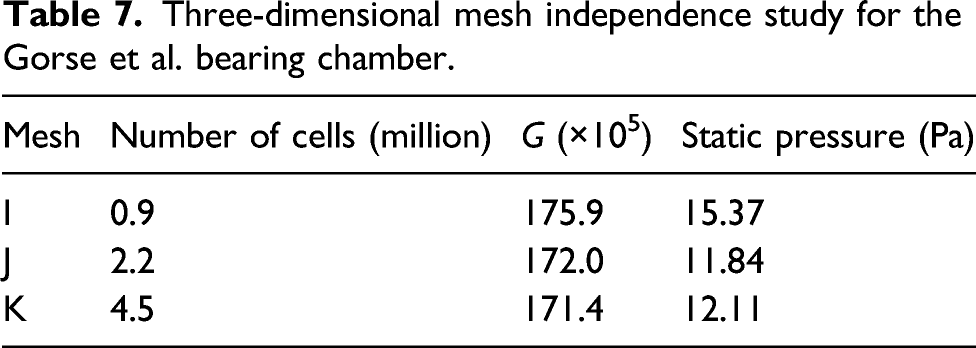
A suitably low mesh dependency was obtained through monitoring non-dimensional torque values and static pressure on the outer cylinder wall; resulting in a percentage difference of less than 1% in the computed non-dimensional torque values and approximately 2% in the static pressure. This mesh is depicted in Figure 10, for which Table 7 presents the computed non-dimensionalised shaft torque, G, and static pressure at H/2 on the outer cylinder wall at the rotational shaft speed of 9700 rpm, which was used to assess mesh independence.

Table 7.

Three-dimensional mesh independence study for the Gorse et al. bearing chamber.

Mesh	Number of cells (million)	G (×10⁵)	Static pressure (Pa)
I	0.9	175.9	15.37
J	2.2	172.0	11.84
K	4.5	171.4	12.11

Operating conditions and fluid properties

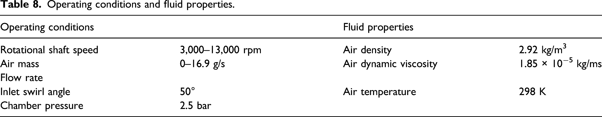
Within the bearing chamber investigation, the operating conditions and fluid properties are derived from the experimental work of Gorse et al.³ and listed in Table 8. Experimentally, the shaft speed is varied between 3000 and 13,000 rpm; however, visualisation results are presented at a shaft speed of 9700 rpm and sealing airflow rates from 4.2 to 16.9 g/s. For all cases investigated, the chamber was kept at a constant pressure of 2.5 bar and an air temperature of 298 K.

Table 8.

Operating conditions and fluid properties.

Operating conditions		Fluid properties
Rotational shaft speed	3,000–13,000 rpm	Air density	2.92 kg/m³
Air mass	0–16.9 g/s	Air dynamic viscosity	1.85 × 10⁻⁵ kg/ms
Flow rate	0–16.9 g/s	Air dynamic viscosity	1.85 × 10⁻⁵ kg/ms
Inlet swirl angle	50°	Air temperature	298 K
Chamber pressure	2.5 bar

Numerical methods and solution procedure

In accordance with the Taylor–Couette investigation, the finite volume incompressible solver, ANSYS Fluent 17.1, was used for all calculations presented. Initial simulations used the SIMPLE algorithm for the pressure–velocity coupling method; however, due to convergence issues, instead, the coupled algorithm was implemented based on the recommendations of Singh et al.¹² The PRESTO discretisation scheme was chosen for the pressure equation and a second order upwinding scheme was used to discretise the remaining equations. For time discretisation, again, a bounded second order implicit temporal discretisation scheme was chosen. After convergence, results were time-averaged for a duration of 0.5 s.

Within bearing chamber applications, the airflow is highly turbulent due to the presence of a rotating shaft throughout the domain, much like a Taylor–Couette flow; however, typically the operational shaft speeds are significantly greater. As such, the previous Taylor–Couette URANS turbulence modelling is extended to the bearing chamber under investigation. The Taylor–Couette study demonstrated that for a full 360° domain, either the standard k-ω or RSM stress-BSL turbulence model was most suited, although it is important to assess whether the conclusions drawn still remain valid, and therefore, a more selective turbulence modelling study is presented.

In addition to the standard k-ω and RSM stress-BSL turbulence model, simulations are also performed for the k-ϵ RNG and SST k-ω turbulence models. For the Taylor–Couette study, all of the investigated ϵ-based turbulence models severely over-predicted both radial and axial velocities. However, for a bearing chamber application, the k-ϵ RNG model has previously been successfully implemented within Volume of Fluid (VOF) investigations such as that demonstrated by Krug et al.¹⁰ Krug et al. reported good prediction of scavenge quantities, although the results for oil distribution were less successful. In addition, the SST k-ω turbulence model has been widely used in bearing chamber applications and is said to represent the state-of-the-art modelling approach, although to date, there has been no attempt to justify this statement.

Bearing chamber operating modes

Within a bearing chamber configuration, Gorse et al.³ report that the secondary airflow vortices can either be categorised into a rotational speed driven mode (RSDM) or a sealing air driven mode (SADM), with a transitional mode occurring between the two. When the sealing airflow rate is small, the RSDM is present, and as the sealing airflow rate is linearly increased, the flow transitions to a SADM. The ratio between the speed of the shaft and sealing airflow can be used to define the transition

R_{v} = \frac{u_{s h}}{u_{a i r}}

(5)

Gorse et al.³ report that when the velocity ratio drops below 4.2, the SADM is present, whereas above which the RSDM dominates. Figures 11(a)–(c) show the secondary flow velocity vectors observed experimentally by Gorse et al.³ for a shaft speed of 9700 rpm. Figure 11(a) highlights the RSDM, with two counter rotating vortices analogous to a Taylor vortex pair; closest to the seal, a slightly larger vortex is observed due to the sealing airflow resulting in the left vortex having an indefinite centre location. As the sealing airflow rate is increased beyond the critical value, the secondary flow pattern begins to transition to a SADM, shown in Figure 11(b); here, the left vortex becomes much smaller and is forced to the upper left-hand corner, such that the vortex separating line no longer resides on the rotor; this is referred to as the transitional mode. Finally, within Figure 11(c), as the sealing airflow rate is increased further, one large dominating vortex is observed due to the strong influence of the sealing airflow causing the left-hand vortex to disappear. Within the bearing chamber, Gorse et al.³ define non-dimensional axial (Z) and radial (Y) positions as

Z = \frac{z}{W} a n d Y = \frac{r}{H}

(6)

where the chamber width is W = 47 mm and the chamber height is H = 44 mm. Here,

z

refers to the axial position and

r

denotes the radial position within the bearing chamber.

Figure 11.

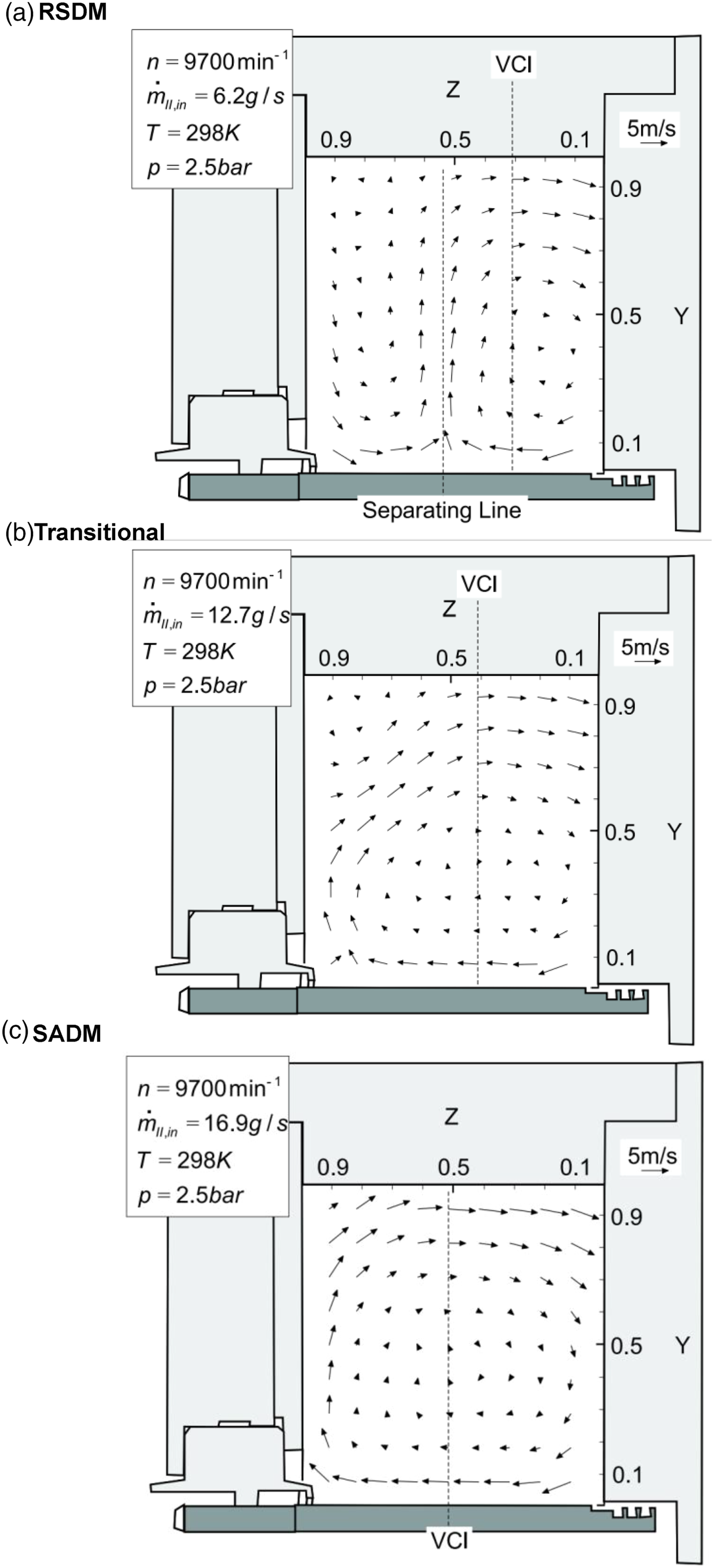
LDA data from Gorse et al.³ showing: (a) RSDM, (b) transitional and (c) SADM secondary flow fields.

In order to benchmark simulations, calculations are therefore first performed without a sealing airflow, to achieve a pure RSDM. After which, the sealing airflow rate is gradually introduced until the flow transitions into a SADM.

Rotational shaft driven mode

Computationally, within the bearing chamber, much like the Taylor–Couette flow, it was observed that the vortical structure is extremely dependent on the initial conditions; even in the absence of a sealing airflow. Initial simulations at moderate shaft speeds, that is, below 9000 rpm failed to reproduce the Taylor vortex-like structure observed experimentally. Instead, depending on the turbulence model employed, either only one large rotating vortex was present or for some cases a vortical structure resembling the SADM, shown in Figure 11(b), was observed. Gorse et al.³ provide no information regarding the start-up conditions employed experimentally, which therefore computationally, becomes extremely difficult in providing a start-up procedure as recommended in the Taylor–Couette study. Therefore, in order to accurately reproduce the flow structure, several different start-up conditions were tested computationally. The results showed that, across all turbulence models, the only case in which a flow structure resembling the RSDM was achieved was when the simulations were first initialised to the highest shaft speed of 13,000 rpm. Subsequently, it was observed, that after the Taylor vortex structure formed and stabilised, it was possible to preserve the structure by reducing the shaft speed in small steps down to 9700 rpm following the optimised start-up procedure methodology outlined within the Taylor–Couette study; here, a small step of 1000 rpm was deemed suitable. Following this technique, the RSDM was preserved and two counter rotating vortices were identified, as shown by the time-averaged velocity vectors Figure 12. Here, as expected, due to the lack of a sealing airflow, two equally sized, counter rotating vortices are observed with distinct vortex centres.

Figure 12.

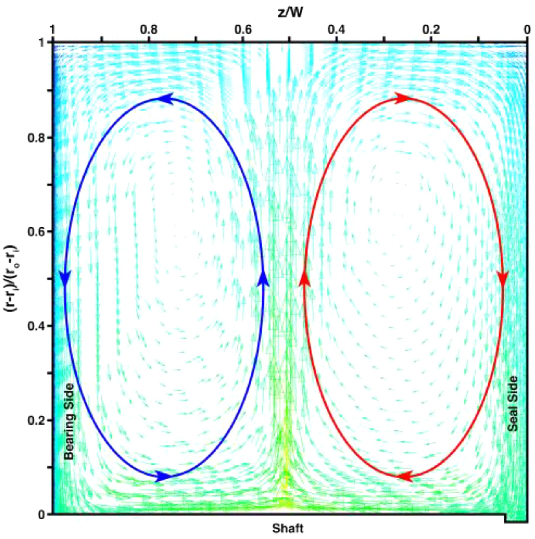
In-plane velocity vectors for RSDM at M_a= 0 g/s and n = 9700 rpm.

Interestingly, over all of the turbulence models investigated, the only case to not reproduce the RSDM was the k-ϵ RNG turbulence model, even at 13,000 rpm. Instead, one large rotating vortex is observed, with a very small counter rotating corner vortex as shown in Figure 13. It is important to consider the formation of this corner vortex, since a sufficient grid resolution close to the wall will be required in order to accurately determine both its shape and size. 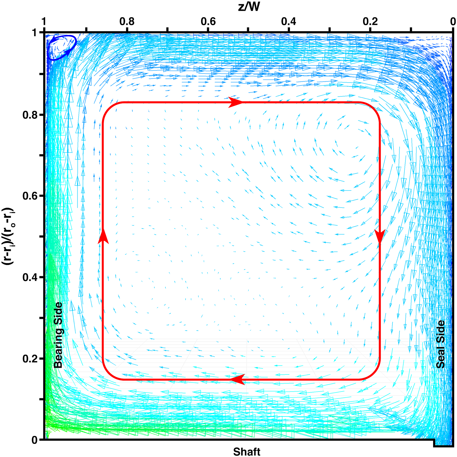The k-ϵ turbulence model can completely fail to predict the effects of corners when very coarse grids near the walls are employed²⁹; however, as shown in Figure 10, care has been taken refine the corners to a value of $y^{+} < 1$ . In general, it was previously determined that the ϵ-based turbulence models were unsuited to model the Taylor–Couette flow investigated earlier, by over predicting both axial and radial velocities. It is surprising that the model fails even to reproduce the Taylor vortex structure within the bearing chamber geometry, especially since the RNG variant is reported to have improved accuracy for flows with rotation and vortices.²⁹

Figure 13.

K-ϵ RNG in-plane velocity vectors for RSDM at M_a= 0 g/s and n = 9700 rpm.

Computationally, once the stable counter rotating vortex pair had formed, at the shaft speed of 9700 rpm, a sealing airflow was subsequently introduced. As the sealing airflow rate is gradually introduced, computationally the right-hand vortex, closest to the seal, gradually increases in size causing the left-hand vortex to diminish in size. The first available experimental measurement point to compare to is at a shaft speed of 9700 rpm and an airflow rate of 6.2 g/s. At this operating condition, all of the turbulence models investigated struggled to fully reproduce the RSDM presented by Gorse et al.,³ as shown in Figure 11(a). Both the standard k-ω and RSM-BSL turbulence models predicted very similar secondary flow patterns, whereby a large, dominating, right-hand vortex forms, with substantially smaller counter-rotating vortices forming at both the top and bottom on the left-hand side of the chamber. This can be seen in Figure 14(a)), which shows the secondary flow field pattern for the RSM stress-BSL turbulence model at 9700 rpm and an airflow rate of 6.2 g/s, an almost identical pattern is seen for the standard k-ω turbulence model. However, this flow field pattern, whilst similar, is still noticeably different to that of the SADM presented by Gorse et al.³ in Figure 11(b). Within Figure 14(a), it can be seen that the vortex separation line still remains attached to the shaft unlike the experimental SADM results.

Figure 14.

(a) RSM stress-BSL and (b) SST K-Ω in-plane velocity vectors for RSDM at M_a= 6.2 g/s and n = 9700 rpm.

The closest agreement found to the RSDM presented by Gorse et al.³ was with the SST k-ω turbulence model, for which the averaged secondary flow field vectors are presented in Figure 14(b). Here, the turbulence model is able to capture the counter rotating Taylor vortex-like structure; however, compared to the results of Gorse et al.,³ a greater right-hand vortex is observed. Experimentally, the vortex separation line occurs at a non-dimensional distance of Z = 0.55, measured from the sealing side of the chamber, whereas computationally, this occurs at the non-dimensional distance of Z = 0.70.

These results are somewhat surprising since both Bristot et al.⁹ and Singh et al.¹² successfully demonstrated the capability to capture the RSDM using the SST k-ω turbulence model on the bearing chamber geometry of Kurz et al.⁶ The bearing chamber employed by Kurz et al. is almost identical to the test rig presented by Gorse et al.³ except that the axial extent of the chamber is 1.4 times longer. Both Bristot et al.⁹ and Singh et al.¹² used the same sealing airflow boundary condition presented in this current computational investigation, using a swirl angle of 50°. For the shaft speed and sealing airflow rate investigated by Bristot et al,⁹ the velocity ratio was $R_{v} = 7.09$ , and conversely, Singh et al.¹² investigated a velocity ratio of $R_{v} = 5.50$ ; for reference, the velocity ratio for the current case operating condition is $R_{v} = 8.59$ . Therefore, the operating spaces investigated by both Bristot et al. and Singh et al. are significantly closer to the transitional state of the flow field, where Gorse et al.³ report that below a value of $R_{v} = 4.2$ , the SADM is present. For the current computational investigation, the numerical methods employed are equivalent to those used by Singh et al.,¹² and it is therefore unexpected as to why, computationally, the SST k-ω turbulence model fails to accurately capture the RSDM, suggesting that the difference in chamber axial length is responsible.

A modified version of the Gorse et al. chamber is presented in Figure 15, in which the bearing chamber is re-meshed with a new axial width of 1.4 times the original chamber width, $W$ , that is, matching the geometry of Kurz et al.⁶ and that investigated numerically by both Bristot et al.⁹ and Singh et al.¹². Figure 15 presents the secondary flow field vectors for the shaft speed of 9700 rpm and 6.2 g/s, using the SST k-ω turbulence model. Therefore, under this operating condition, the flow is within the RSDM with $R_{v} = 8.59$ . Under these flow conditions, a clear counter rotating Taylor vortex-like structure is observed. A slightly larger vortex is identified closer to the sealing side, due to the presence of the sealing airflow. This results in the vortex separation line located at the non-dimensional distance of approximately 7.5, noting that the domain axial length extends to the non-dimensional distance of 1.4. Compared to Figure 11(a), the numerical results are in agreement with the visualisation vectors presented by Gorse et al,³ in which the vortex separation line is located just off-centre due to the presence of a slightly larger sealing-side vortex.

Figure 15.

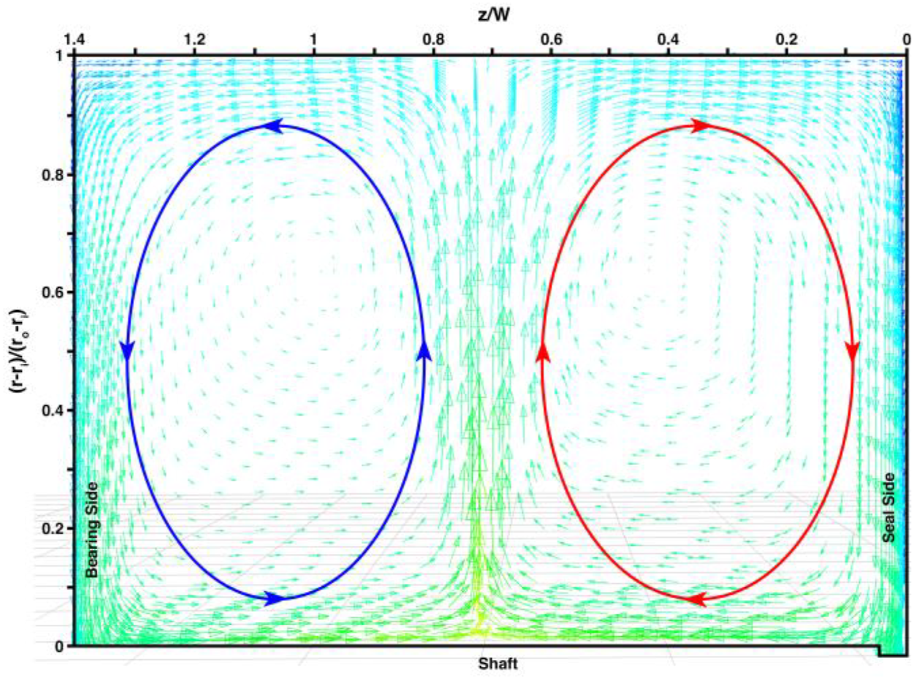
In-plane velocity vectors for RSDM at M_a= 6.2 g/s and n = 9700 rpm, for the chamber geometry of Gorse et al.³ modified to an axial width of 1.4 W.

Overall, the results clearly demonstrate that due to the increased chamber axial length, the SST k-ω turbulence model is able to predict the RSDM, suggesting that the location of the vortex separation line is very sensitive to the sealing airflow input. By extending the chamber axial length, at the chamber centreline location, the same sealing airflow rate will be relatively weaker, causing the shaft rotation to drive the flow field. However, with the reduced chamber length, the same sealing airflow rate causes the vortex centreline location to be pushed further axially into the chamber.

Transitional mode

As the sealing airflow rate is increased, the flow state transitions from a RSDM to that of a SADM; Gorse et al.³ show that this first starts to take place at an airflow rate of 12.7 g/s, as shown in Figure 11(b). Experimentally, at this flow rate, the vortex separating line becomes detached from the rotor surface and moves up the bearing chamber left-hand wall. At a shaft speed of 9700 rpm and an airflow rate of 12.7 g/s, this separation line occurs at the non-dimensional radial distance of R = 0.60 from the shaft. As a result, the left-hand vortex reduces in size significantly and is forced into the top left corner of the bearing chamber, with the vortex centre located at the non-dimensional location R = 0.90 and Z = 0.88.

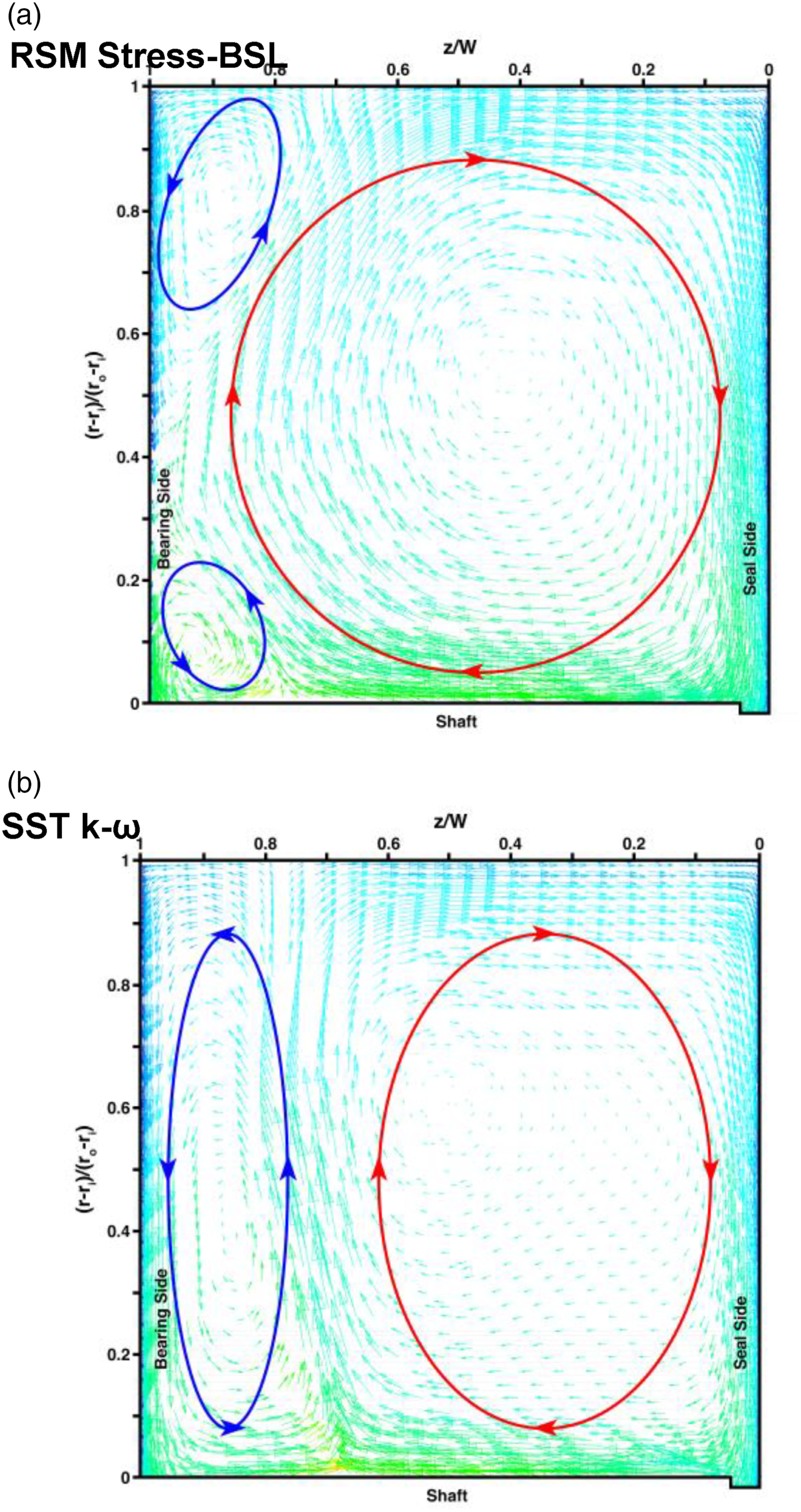
Figure 16 shows the averaged secondary flow field vectors for each of the turbulence models investigated at a shaft speed of 9700 rpm and a sealing airflow rate of 12.7 g/s. The results for the k-ϵ RNG turbulence model are not shown since under these operating conditions, there was no change in the secondary flow field and an identical vortex structure as previously shown in Figure 13 was observed. Overall, within the bearing chamber geometry, the k-ϵ RNG turbulence model completely failed to capture the flow field patterns reported by Gorse et al.³ over all of the shaft speeds and airflow rates investigated and is therefore not shown.

Figure 16.

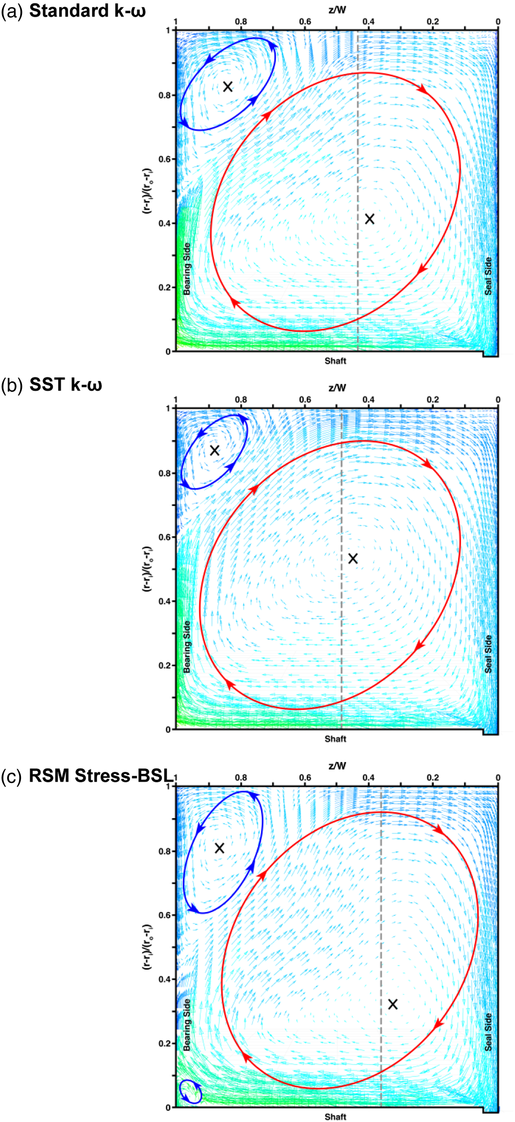
In-plane velocity vectors for the transitional state at M_a= 12.7 g/s and n = 9700 rpm a) Standard k-omega turbulence model, b) SST k-omega turbulence model, c) RSM Stress-BSL turbulence model.

Figure 16(a) shows the results of the standard k-ω turbulence model; here, the transitional mode is fully captured with the vortex separating line occurring at the non-dimensional location R = 0.47. As a result, a slightly larger corner vortex is observed when compared to the experimental results of Gorse et al.³ Similarly, the results of the SST k-ω turbulence model are shown in Figure 16(b). With the SST k-ω turbulence model, a closer agreement to the experimental data is observed, with the vortex separating line located at R = 0.61, and therefore, a similar sized vortex is found at the top left corner of the chamber. Finally, the results of the RSM stress-BSL turbulence model are shown within Figure 16(c)). Here, whilst a comparable transitional vortex structure is observed, visually, the most noticeable difference is the presence of two vortex separation lines, one located at R = 0.44 and the second attached to the shaft at Z = 0.9.

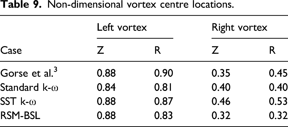
Table 9 summarises the centre location of the each of two main vortices compared to the results of Gorse et al.³ The axial location of the left-hand vortex remains fairly consistent over all of the turbulence models investigated; however, the greatest difference lies within the radial co-ordinate, resulting from the difference in separation lines and hence the vortex size as previously discussed. The closest agreement to the experimental data is found with the SST k-ω turbulence model; however, when considering the right-hand vortex, all of the turbulence models showed a much greater variation from the experiment, with percentage difference in the region of 20%.

Table 9.

Non-dimensional vortex centre locations.

	Left vortex		Right vortex
Case	Z	R	Z	R
Gorse et al.³	0.88	0.90	0.35	0.45
Standard k-ω	0.84	0.81	0.40	0.40
SST k-ω	0.88	0.87	0.46	0.53
RSM-BSL	0.88	0.83	0.32	0.32

Under these operating conditions, Figure 17 shows the non-dimensional radial profiles of the mean tangential velocity at the axial positions defined by the dashed line within Figures 16(a)–(c). The axial locations are taken just off-centre of the right-hand vortex, in line with the experimental method presented by Gorse et al.³ Across all cases, the mean tangential velocity is non-dimensionalised by the shaft speed. Whilst the transitional mode was not achieved using the k-ϵ RNG turbulence model, a comparison is also made.

Figure 17.

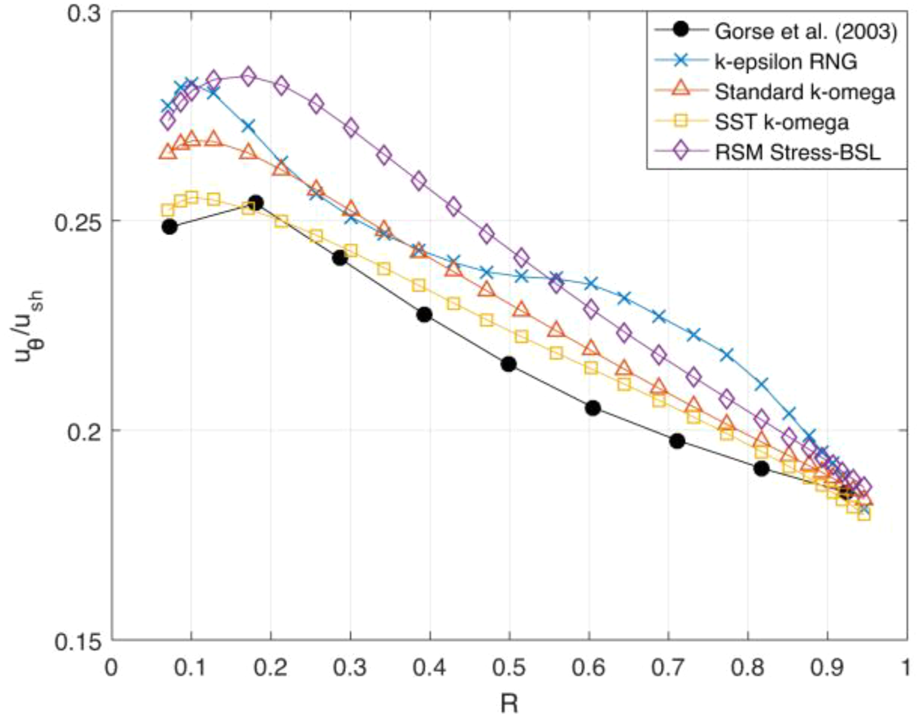
Radial profiles of non-dimensional tangential velocity at M_a= 12.7 g/s and n = 9700 rpm.

Within Figure 17, it is clear that across all of the turbulence models investigated, the SST k-ω turbulence model provides the closest agreement to the experimental measurements. This can be associated with the model’s ability to accurately capture the secondary flow field as evident in the comparison to the LDA data of Gorse et al.³ For the SST k-ω turbulence model, the greatest discrepancy occurs over the non-dimensional radial distance of R = 0.4 to R = 0.8; however, over this range, the maximum percentage difference in the tangential velocity was less than 5%. In contrast, the RSM stress-BSL model produced the greatest deviations from the experimental measurements, with a maximum percentage difference of 12%, occurring at R = 0.18.

The recommended turbulence modelling methodology presented in the Taylor–Couette study suggested that the most appropriate models were either the standard k-ω or RSM stress-BSL. However, it was noted that whilst the SST k-ω model predicted very similar velocity profiles to the standard k-ω model, the biggest difference occurred within the axial wavelength of the Taylor vortex pairs. For the SST k-ω model, the size of the Taylor vortices was approximately 5% larger, resulting in smaller end cells. Within a bearing chamber, due to the constrained axial length of the geometry, this phenomenon does not present a problem since the space only permits a single vortex pair to form. Surprisingly, the RSM stress-BSL model, unlike in the Taylor–Couette study, performed quite poorly especially when comparing velocity profiles. In addition, due to the more complex nature of the RSM formulation, as expected, simulations were considerably more expensive; numerically taking up to five times as long to reach the same flow time, compared to the two-equation models. As such, for the bearing chamber geometry under investigation, it is clear that both quantitatively and qualitatively the SST k-ω model is the most suitable URANS turbulence model.

Sealing air driven mode

As the sealing airflow rate is increased further, the flow state moves fully into that of a SADM; the LDA results of Gorse et al.³ demonstrate this at an airflow rate of 16.9 g/s, as shown in Figure 11(c). Experimentally, at this flow rate, the presence of counter-rotating vortices is completely wiped out and the flow is driven by one large vortex due to the dominance of the sealing airflow. Figure 18 presents the averaged secondary flow field vectors using the SST k-ω turbulence model for the shaft speed of 9700 rpm and 16.9 g/s. Much like the experimental visualisation results in Figure 11(c), numerically one large dominating vortex is observed; however, two smaller corner vortices are observed at the top left-hand and right-hand locations. The recognition of these corner vortices is important for bearing chamber investigations; their size and shape may heavily depend on the grid resolution and therefore may require further refinement to accurately capture. Within a bearing chamber, a thin oil film will form on this top wall that is, the outer casing wall, and these vortices may influence the oil film distribution. For example, the top left-hand vortex will push oil away from the centre of the outer casing wall toward the left-hand chamber wall. Subsequently, this will result in the oil film being redistributed away from the sump. Conversely, the presence of a thick oil film, which can have a length scale in mm, for example, 1–2 mm demonstrated by Bristot et al,⁹ can completely wipe out these corner vortices as highlighted by the in-plane velocity vectors of Bristot et al,⁹ in which the VOF iso-surfaces of oil are also superimposed.

Figure 18.

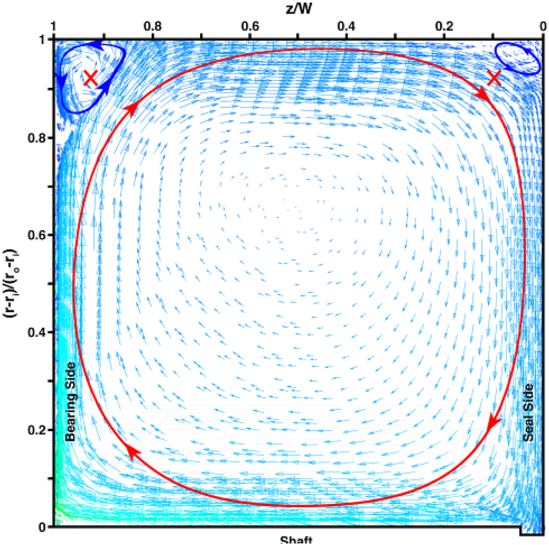
In-plane velocity vectors for SADM at M_a= 16.9 g/s and n = 9700 rpm.

In general, it is suspected that the resolution of the LDA method employed by Gorse et al³ may not capture these corner vortices. For example, within Figure 11(c), the visualisation images of Gorse et al.³ only depict one large dominating vortex, with no corner vortices. However, in Figure 11(c), the top-most left-hand measurement point is 3.5 mm away from the side wall and 3.5 mm from the top wall; similarly, the top right-hand measurement point is 4.5 mm away from the side wall and 3.5 mm from the top wall. These measurement locations are indicated by the red crosses in Figure 18. Close inspection shows that at these measurement locations the flow is travelling in the same direction as that depicted in Figure 11(c), This suggests that the numerical results are in good agreement with the LDA data of Gorse et al.³

Variation in shaft speed

Based on the results achieved throughout the RSDM and SADM, the effect of varying the shaft speed on the secondary airflow field is explored using the SST k-ω turbulence model, for a fixed airflow rate of 12.7 g/s. Due to the difficulties of reproducing the counter rotating Taylor vortex-like structure within the RSDM, a higher sealing airflow rate is investigated; however, the RSDM parameter space is still explored. The main reason for this is due to the lack of available experimental data to compare to, both qualitatively and quantitatively, since Gorse et al.³ only presents results at a fixed shaft speed of 9700 rpm. Numerically, the rotational shaft speed is varied from 3000; 6000; 9700 and 13,000 rpm, which corresponds to velocity ratios of $R_{v} = 1.30; 2.59; 4.19 a n d 5.60$ , respectively, noting that for values of $R_{v}$ less than 4.2, Gorse et al.³ report that the SADM is present.

Figures 19(a)–(d) show the secondary flow field vectors for each of the corresponding shaft speeds investigated. Figures 19(a) and (b) represent the SADM, where one large central vortex is observed, and two smaller corner vortices form. Between Figures 19(a) and (b), some difference in the size of these corner vortices is observed, but largely, the overall flow field is very similar. Compared to Figure 18, which demonstrated good agreement for the SADM with the experimental visualisation of Gorse et al,³ Figures 19(a) and (b)) present a similar secondary flow field structure; however, again some differences are observed in the size and shape of these corner vortices. The top-most left-hand and right-hand LDA measurement locations for Figure 11(c), as previously discussed, are depicted by the red crosses in Figures 19(a) and (b)). At these measurement locations, the centre location of the corner vortices lies closer to the wall than these LDA points. As such, when comparing the direction of the numerical secondary flow field velocity vectors with that of the vectors of Gorse et al,³ in Figure 11(c)), the results are in good agreement.

Figure 19.

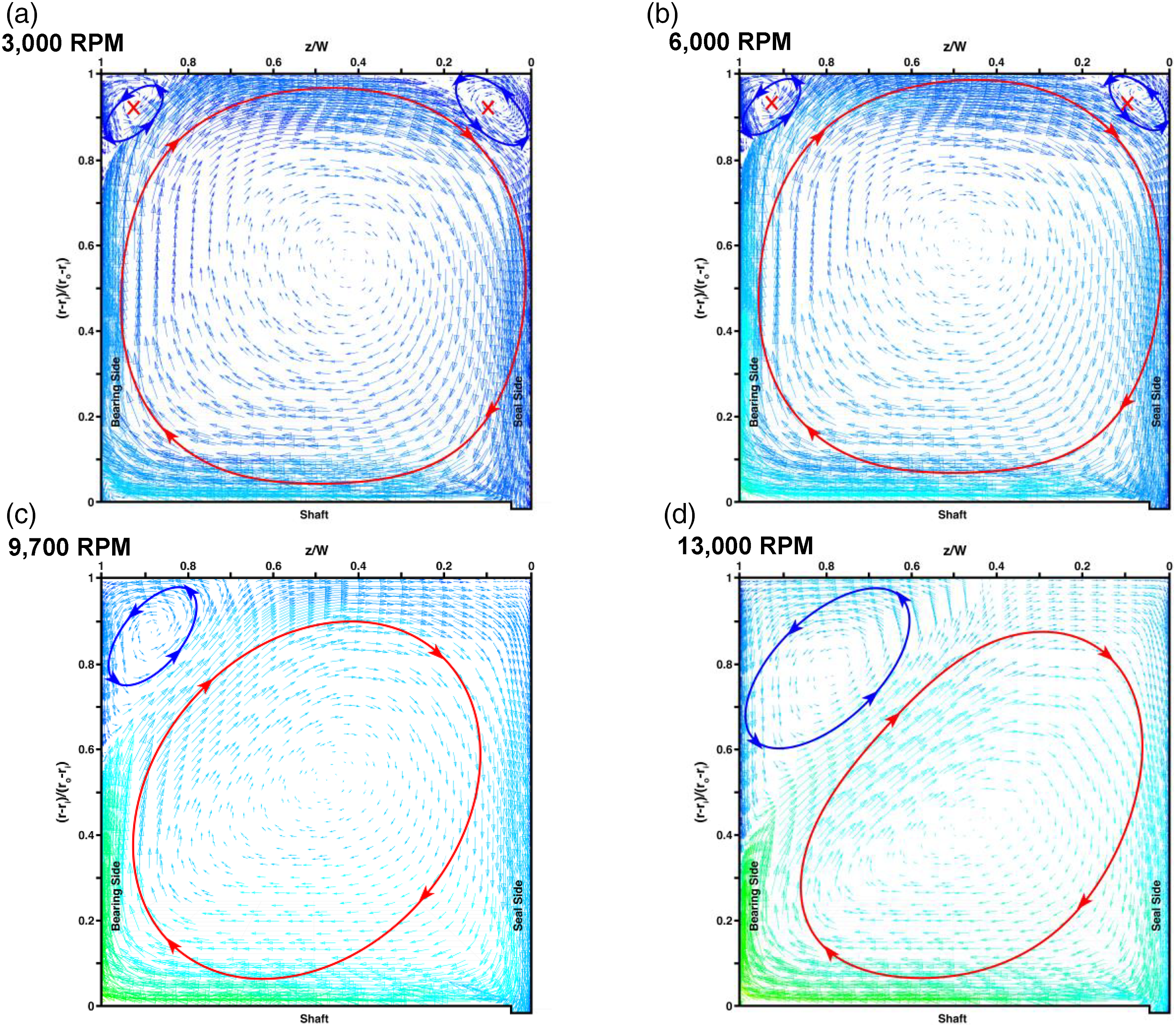
In-plane velocity vectors for different shaft speeds at M_a= 12.7 g/s: (a) 3000 rpm, (b) 6000 rpm, (c) 9700 rpm and (d) 13,000 rpm.

Figure 19(c) represents the transitional mode previously investigated in Figure 16(b), whereby the transition from the SADM to the RSDM is beginning to take place. Here, the vortex separation line becomes attached to the bearing chamber left-hand wall instead of the rotor surface. As shown previously, good agreement with the experimental data is observed both visually and quantitatively at this shaft speed.

Finally, as the shaft speed is increased to 13,000 rpm, shown in Figure 19(d), the velocity ratio $R_{v} = 5.60$ , suggesting that the flow state should be within the RSDM. However, from the experimental results of Gorse et al,³ it is unclear whether the flow field at this velocity ratio has fully transitioned to the RSDM, where the vortex separation line resides on the surface of the shaft. For example, from the results of Gorse et al.,³ at 9700 rpm and 12.7 g/s, $R_{v} = 4.19$ , and as shown in Figure 11(b), transition is taking place. At 9700 rpm and 8.5 g/s, $R_{v} = 6.26$ , and Gorse et al.³ observe the RSDM, with the separation line attached to the shaft surface; under these conditions, the sealing-side vortex is bigger than the bearing side vortex. Subsequently, at 9700 rpm and 6.2 g/s, $R_{v} = 8.59$ , and as shown in Figure 11(a), two almost equal size counter rotating vortices are observed. Numerically, at 13,000 rpm and 12.7 g/s, $R_{v} = 5.60$ , and therefore, the operating condition lies in-between the two investigated points of Gorse et al,³ where at $R_{v} = 4.19$ , transition is taking place, and at $R_{v} = 6.26$ , the RSDM is observed. Therefore, it is unclear at these operating conditions, which secondary flow field is expected. From Figure 19(d), the secondary flow field is clearly within the transitional state, and the vortex separation line is attached to the left-hand bearing chamber wall. Compared to Figure 19(c), within Figure 19(d), the left-hand vortex is however larger, suggesting that the flow is beginning to approaching the RSDM.

Conclusion

Axisymmetric and three-dimensional CFD modelling of Taylor–Couette flow within the turbulent Taylor vortex flow regime was analysed and compared to available experimental data with a view to establishing a methodology applicable to future bearing chamber modelling. The conclusions are as follows:

• Start-up: An optimised steady acceleration start-up is indicated for future modelling. An investigation was performed into the start-up procedure. Sudden starts of the inner cylinder were compared to results obtained following a steady acceleration procedure. Through sudden starts, a large variation in the wavelength of Taylor vortices was obtained, resulting in different configurations in the number of Taylor vortex pairs. However, through a steady acceleration procedure, it was possible to achieve a final desired state over the whole range of rotational Reynolds number ratios investigated. Once the Taylor vortices form and stabilise after a steady acceleration procedure, it is then possible to increase the speed of the inner cylinder in small steps whilst still preserving the same number of Taylor vortex pairs, allowing the computational cost of simulations to be reduced over accelerations to large rotational Reynolds numbers.

• Axisymmetric modelling: Axisymmetric modelling is inadequate for bearing chamber modelling. An axisymmetric URANS turbulence modelling study was performed on an axisymmetric grid. Good agreement was obtained for both the standard k-ω and RSM stress-BSL turbulence models at low rotational Reynolds number ratios. However, it was observed that as the speed of the inner cylinder is increased, the agreement between CFD and experimental results became poor. This is suspected to be as a result of not capturing the three-dimensional structures present within turbulent Taylor–Couette flow, such as boundary layer Görtler vortices.

• Three-dimensional modelling with rotational periodicity: Rotational periodicity is unlikely to be adequate for bearing chamber modelling. The axisymmetric CFD methodology was extended to modelling in three-dimensions building on the previous knowledge acquired. A study into applying rotational periodicity was carried out in order to reduce the computational cost. Poor agreement was achieved over all of the rotational periodicities investigated. The radial velocity profiles were overestimated, and a much-reduced core velocity was observed when comparing the velocity magnitude across the gap.

• Recommended methodology: A full 360° model with either the standard k-ω or RSM stress-BSL turbulence model is recommended for the bearing chamber study. Finally, the full $360 °$ geometry was modelled. The results showed negligible difference between the standard k-ω and RSM turbulence models; however, good agreement was achieved with the experimental PIV data of Wang²² and the hot-wire data presented by Smith and Townsend.²⁷ These results show that it is possible to accurately capture the velocity flow field within 5% with URANS turbulence modelling through simulating the full $360 °$ geometrical domain using either the standard k-ω or RSM stress-BSL turbulence models. For industrially relevant flows, either turbulence model is suitable; however, the RSM is more computationally expensive but has the advantage of being anisotropic, hence turbulence statistics are readily available.

Subsequently, the three-dimensional Taylor–Couette turbulence modelling methodology has been expanded and applied to a bearing chamber geometry. Numerical studies are conducted over a range of shaft speeds and sealing airflow rates. A qualitative and quantitative analysis of the secondary airflow structure is carried out and compared to the experimental measurements of Gorse et al.³ Initial calculations determined that it was necessary to include a start-up procedure, as highlighted by the Taylor–Couette study. As such, simulations were first initialised to 13,000 rpm after which the rotational shaft speed was reduced in small steps to the final desired state.

Qualitatively, without a sealing airflow, all of the turbulence models investigated were able to fully capture the RSDM, except for the k-ϵ RNG model. For all of the experimental operating conditions investigated, the k-ϵ RNG turbulence model performed poorly producing only one large rotating vortex structure. At low sealing airflow rates, all of the turbulence models struggled to capture the RSDM presented by Gorse et al.³ The closest agreement was found with the SST k-ω turbulence model although compared to the experimental measurements, a larger than expected right-hand vortex was observed. At moderate sealing airflow rates, the transitional mode was predicted well by both the standard/SST k-ω models and also by the RSM stress-BSL turbulence model, all accurately capturing the vortical structure presented by Gorse et al.³

Quantitatively, at the transitional mode, a comparison of vortex central locations revealed good agreement across all of the turbulence models. For the left-hand vortex location, the closest agreement was achieved using the SST k-ω turbulence model, as a result of accurately capturing the vortex separation line. However, for all of the cases investigated, the central location of the right-hand vortex was not captured well. Normalised tangential velocity profiles radially across the gap were also compared to the available measurements of Gorse et al.³ Again, out of all of the turbulence models investigated, the closest agreement was observed for the SST k-ω turbulence model, with local percentage differences no greater than 5%. Surprisingly, the poorest agreement was found with the RSM stress-BSL model, with percentage differences as large as 12%.

Within the SADM, the SST k-ω turbulence model was able to accurately reproduce the secondary flow field observed visually, demonstrating one large dominating vortex. Numerically, two counter rotating corner vortices are identified at the top of the chamber. These are not identified experimentally due to the resolution of the LDA measurement locations. Finally, the effect of varying the shaft speed on the secondary flow field is investigated at a fixed sealing airflow rate, highlighting the transitional process from the SADM to the RSDM.

The results of the bearing chamber investigation differ slightly to that of the Taylor–Couette study. Within the Taylor–Couette methodology, the standard k-ω and RSM stress-BSL turbulence models were recommended as the most suitable choices; although for the bearing chamber investigations, the best results were achieved using the SST k-ω turbulence model. The Taylor–Couette modelling revealed that whilst similar to the standard k-ω model, the SST k-ω model over predicted the vortex axial wavelengths. However, it is clear that within a bearing chamber geometry, this is not as significant, due to the constrained chamber axial length. Overall, a good agreement is instead presented with the SST k-ω model.

The present work has demonstrated the performance of URANS turbulence modelling applications to a bearing chamber geometry, benchmarking the performance of different turbulence modelling approaches. The best practical approach for bearing chamber applications is the SST k-ω turbulence model. As such, the SST k-ω turbulence model is recommended for all future bearing chamber simulations. Due to the sensitivity of the secondary flow field, numerically, procedures should be taken to reproduce the start-up conditions employed experimentally.

Footnotes

Acknowledgements

The authors are grateful for access to the University of Nottingham High Performance Computing Facility. In addition, the authors acknowledge the use of Athena at HPC Midlands+, which was funded by the EPSRC on grant EP/P020232/1.

Declaration of conflicting interests

The author(s) declared no potential conflicts of interest with respect to the research, authorship, and/or publication of this article.

Funding

The author(s) disclosed receipt of the following financial support for the research, authorship, and/or publication of this article: This work was supported by the Engineering and Physical Sciences Research Council grant number EP/P020232/1.

ORCID iD

Kathy Johnson

Appendix

References

Nicoli

Johnson

Jefferson-loveday

. Simulation of a simplified aeroengine bearing using a fully coupled two-way eulerian thin film/discrete phase approach part I: film behaviour near the bearing. J Eng Gas Turbines Power 2021; 140(10): 101015.

Nicoli

Johnson

Jefferson-loveday

. Simulation of a simplified aeroengine bearing using a fully coupled two-way eulerian thin film/discrete phase approach part II: droplet behaviour in the chamber. J Eng Gas Turbines Power 2021; 143(10): 101016.

Gorse

Willenborg

Busam

, et al. 3D-LDA measurements in an aero-engine bearing chamber. Proc ASME Turbo Expo 2003; 5: 257–265.

Gorse

Busam

Dullenkopf

. Influence of operating condition and geometry on the oil film thickness in aeroengine bearing chambers. J Eng Gas Turbines Power 2004; 128(1): 103–110.

Lee

. Air and oil flow investigations in an aeroengine bearing chamber. PhD Thesis. Nottingham, UK: University of Nottingham, 2004.

Kurz

Bauer

H-J

. An approach for predicting the flow regime in an aero engine bearing chamber. Proc ASME Turbo Expo 2014; 5C: 1–8.

Glahn

Kurreck

Willmann

, et al. Feasibility study on oil droplet flow investigations inside aero engine bearing chambers—PDPA techniques in combination with numerical approaches. J Eng Gas Turbines Power 1996; 118(4): 749–755.

Gorse

Dullenkopf

Bauer

H-J

, et al. An experimental study on droplet generation in bearing chambers caused by roller bearings. Proc ASME Turbo Expo 2008; 43147: 1681–1692.

Bristot

Morvan

Simmons

. Evaluation of a volume of fluid CFD methodology for the oil film thickness estimation in an aero-engine bearing chamber. Proc ASME Turbo Expo 2016; 2C: 1–11.

10.

Krug

Höfler

Bauer

H.-J.

, et al. Evaluation of the volume-of-fluid method for the numerical modelling of an aero engine bearing chamber. In: 22nd International Symposium on Air Breathing Engines (ISABE 2015), Phoenix, AZ, 25–30 October 2015, 2015.

11.

Singh

Sharabi

Ambrose

, et al. Assessment of an enhanced thin film model to capture wetting and drying. In: ASME Turbo Expo 2019: Turbomachinery Technical Conference and Exposition, Phoenix, AZ, 17–21 July 2019, 2019.

12.

Singh

Sharabi

Ambrose

, et al. Prediction of film thickness of an aero-engine bearing chamber using coupled VOF and thin film model. In: ASME Turbo Expo 2019: Turbomachinery Technical Conference and Exposition, Phoenix, AZ, 17–21 July 2019, 2019.

13.

Peduto

Hashmi

Dullenkopf

, et al. Modelling of an aero-engine bearing chamber using enhanced CFD technique. In: ASME 2011 Turbo Expo: Turbine Technical Conference and Exposition, Vancouver, BC, 6–10 June 2011, 2011, pp. 809–819.

14.

Farrall

Hibberd

Simmons

. The effect of initial injection conditions on the oil droplet motion in a simplified bearing chamber. J Eng Gas Turbines Power 2008; 130(1): 1–7.

15.

Aidarinis

Missirlis

Yakinthos

, et al. CFD modeling and LDA measurements for the air-flow in an aero engine front bearing chamber. J Eng Gas Turbines Power 2011; 133(8): 82504–82508.

16.

Aidarinis

Goulas

. Enhanced computational fluid dynamics modeling and laser doppler anemometer measurements for the air-flow in an aero-engine front bearing chamber—part I. J Eng Gas Turbines Power 2015; 137(8): 082501.

17.

Peduto

. Oil droplet impact dynamics in aero-engine bearing chambers-correlations derived from direct numerical simulations. PhD Thesis. Karlsruhe, Germany: Karlsruhe Institute of Technology, 2015.

18.

Wild

Djilali

Vickers

. Experimental and computational assessment of windage losses in rotating machinery. J Fluids Eng 1996; 118(1): 116–122.

19.

Adebayo

Rona

. The Three-Dimensional Velocity Distribution of Wide Gap Taylor-Couette Flow Modelled by CFD. Int J Rotating Mach 2016; 2016(2): 1–11.

20.

Adebayo

Rona

. Numerical investigation of the three-dimensional pressure distribution in Taylor couette flow. J Fluids Eng 2017; 139(11): 111201–111210.

21.

Batten

WMJ

Bressloff

Turnock

. Transition from vortex to wall driven turbulence production in the Taylor–Couette system with a rotating inner cylinder. Int J Numer Method Fluid 2002; 38(3): 207–226.

22.

Wang

. Computational fluid dynamics simulation of precipitation processes. PhD Thesis. Ames, IA: Iowa State Univesity, 2004.

23.

Coles

. Transition in circular Couette flow. J Fluid Mech 1965; 21(3): 385–425.

24.

Koschmieder

. Turbulent Taylor vortex flow. J Fluid Mech 1978; 93(3): 515–527.

25.

Poncet

Da Soghe

Bianchini

, et al. Turbulent Couette-Taylor flows with endwall effects: a numerical benchmark. Int J Heat Fluid Flow 2013; 44: 229–238.

26.

Burin

Schartman

. Local measurements of turbulent angular momentum transport in circular Couette flow. Exper Fluid 2010; 48: 763–769.

27.

Smith

Townsend

. Turbulent Couette flow between concentric cylinders at large Taylor numbers. J Fluid Mech 1982; 123: 187–217.

28.

Donnelly

Schwarz

Roberts

. Experiments on the stability of viscous flow between rotating cylinders. Proc R Soc A 1964; 283: 531–556.

29.

ANSYS . ANSYS FLUENT Theory Guide Release 17.1. Canonsburg: ANSYS, 2016.

30.

Versteeg

Malalasekera

. Introduction: Computational Fluid Dynamics the Finite Volume Method. London, UK: Pearson Education, 2006.

31.

Barcilon

Brindley

Lessen

, et al. Marginal instability in Taylor-Couette flows at a very high Taylor number. J Fluid Mech 1979; 94(3): 453–463.

32.

Brauckmann

Eckhardt

. Direct numerical simulations of local and global torque in Taylor-Couette flow. J Fluid Mech 2013; 718: 398–427.

33.

Ostilla-Mónico

Verzicco

Lohse

. Effects of the computational domain size on direct numerical simulations of Taylor-Couette turbulence with stationary outer cylinder. Phys Fluids 2015; 27(2): 25110.

Computational modelling of turbulent Taylor–Couette flow for bearing chamber applications: A comparison of unsteady Reynolds-averaged Navier–Stokes models

Abstract

Keywords

Introduction

Taylor–Couette studies

Objectives

Taylor–Couette investigations

Numerical methods

Unsteady Reynolds-averaged Navier–Stokes turbulence modelling

Axisymmetric modelling

Start-up procedure

Unsteady Reynolds-averaged Navier–Stokes turbulence modelling

Three-dimensional modelling

Start-up procedure

Rotational periodicity study

Three-dimensional results

Bearing chamber investigations

Boundary conditions and mesh

Operating conditions and fluid properties

Numerical methods and solution procedure

Bearing chamber operating modes

Rotational shaft driven mode

Transitional mode

Sealing air driven mode

Variation in shaft speed

Conclusion

Footnotes

Acknowledgements

Declaration of conflicting interests

Funding

ORCID iD

Appendix

References