
Abstract
Gas turbine performance models typically rely on component maps to characterize engine component performance throughout the operational regime. For the sub-idle case, the lack of reliable rig test data or inability to run design codes far from design conditions entails that component maps have to be generated from the extrapolation of existing data at higher speeds. This undermines the accuracy of whole-engine sub-idle performance models, at times impacting engine development and certification of aviation engines and the accuracy of start-up performance prediction in industrial gas turbines. One of the main components driving this issue is the core compression system, which can present operability concerns during light-up and which also sets the combustor airflow required for ignition. This paper presents, discusses, and draws on previous approaches to describe a method enabling the creation of sub-idle compressor maps from analytical and physical grounds. The method relies on the calculation of zero-speed and torque-free lines to generate a map down to zero speed along with analytical interpolation. A method for the interpolation process is described. A sensitivity study is carried out to assess the effects that different elements of the map generation process may have on the accuracy of the resulting performance calculation. Overall, a method for the generation of accurate, consistent maps from limited geometry data is identified.
Introduction
Stringent end-user requirements on the relight capabilities of aviation engines mean that designers must be able to accurately predict the engine’s behavior during in-flight relight events.1 In addition, the drive towards improved efficiency and lower fuel burn means that the design for ground-starts and long taxi periods, operating at low speed, must be taken into account, increasing the need for performance optimization at and below idle. On the power generation front, the current drive towards distributed generation, a more diverse energy mix, and increasing reliance on intermittent renewable energy sources may require gas turbine peaking power plants to meet demand. As opposed to large frame GT and GTCC power plants operating in a base-load capacity, “peaker” units will go through multiple cycles of start-up and shut down, making start-up performance and dispatch times increasingly important. In both aviation and industrial power generation cases, improved sub-idle performance prediction capability is required.
In order to use gas turbine performance solvers to predict start-up and relight behavior, engine component maps covering very low-speed regions must be available. The axial compressor is of special importance due to operational limitations related to stall and surge. Hence, this work presents a method to obtain consistent axial compressor sub-idle maps based on physical arguments and models. Compressor maps have traditionally been obtained from rig tests. Obtaining compressor maps in this manner for sub-idle regions is expensive and impractical, as a means to control the shaft torque while providing different mass flows to the compressor rig would be required, instead of letting the compressor set the flow upon operation.2 Furthermore, instrumented development engines would require a different set of instrumentation for sub-idle operation, with added complexity and cost implications. More recently, it has become possible to generate predicted compressor maps for new compressor designs using aerodynamic design codes, however these are most accurate near design conditions and may become inaccurate or not run at all under sub-idle conditions. In order to obtain maps for which there is little experimental data, analytical map extrapolation methods are used, but these typically rely on trends and rules which might not be applicable in the sub-idle region.3 Map extrapolation has traditionally relied on a combination of graphical methods, past-experience, and engineering judgement.4 Such methods become problematic far below the idle speed, where limited data exists.5
Literature review
The method developed here builds on previous map generation approaches that have appeared in the literature over the last decades. These previous approaches are discussed below. The highlights and limitations of these existing approaches are presented, showing how the method presented here seeks to improve on them. A brief discussion on sub-idle performance parameters is also provided. The existing work on the windmill performance of fans is also reviewed here, since fundamental concepts from this topic are implemented in the map generation method developed.
Previous methods for sub-idle map extension
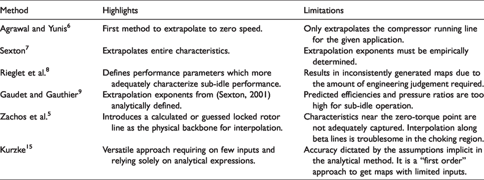
In order to calculate compressor starting behavior, Agrawal and Yunis6 devised a methodology making use of incompressible flow similarity relations to generate the start-up running line. Such an approach was later expanded by Sexton7 to generate entire characteristics through extrapolation based on similarity laws and empirically obtained exponents. Around the same time, Riegler et al.8 discussed the need to use a different set of performance parameters to characterize sub-idle performance, such as the use of torque in place of efficiency. That work also presented a method for graphically generating maps to zero speed which, although practical, did not produce consistent maps due to the amount of user judgement and manipulation required. Gaudet and Gauthier9 later expanded on Sexton’s approach by including analytical expressions for the extrapolation exponents, but did not implement any of the recommendations from Riegler et al.8 The method is consistent and straightforward but fails to produce maps that capture overall loss that may be present at sub-idle and results in efficiencies that are much too high for the conditions under consideration.10
A physically enhanced method for the generation of sub-idle maps was presented by Zachos et al.5,11 relying on interpolation up to idle from an analytically generated locked rotor line, i.e. zero speed characteristic. This would enhance the method of Gaudet and Gauthier9 by allowing pressure ratios below unity and by generating low speed lines which more closely resemble the physical operation of compressors operating at very low speeds. The method also included some of the recommendations from Riegler et al.8 by using torque in place of efficiency. The method involves interpolation along artificial “beta lines” which serve as coordinates tying points on different characteristics together. This method has been used to generate compressor maps down to zero speed which capture the expected trends5,12 and have successfully been used in performance models.13,14 It was later shown10 that this interpolation method relying only on the locked rotor line did not accurately capture torque-free windmilling points obtained from a rig test, so the addition of more sub-idle points, such as an analytically generated torque-free windmill line, to the interpolation process was proposed. In addition, the interpolation along artificially defined “beta lines” adds another user input that can impact results, since these are not defined by any physical means and are essentially “drawn” visually on the map. This especially true near the choke region, where characteristics become vertical.
Most recently, Kurzke15 identified an approach for map generation to zero speed for the case where absolutely no geometry data is available. A practical approach is presented where empirical relationships regarding the slope of the torque characteristic and engineering judgement regarding flow conditions at the compressor OGV are used to extend compressor map to zero speed. Kurzke’s method is implemented in the well-known SmoothC program,4 as an improvement to the method in Riegler et al.8 The resulting map can then be smoothed as required to ensure a physical outcome.
All these map generation methods have built on one another, but a consistent, physics-based approach that accurately captures all physical trends without the need for extensive user judgement does not appear to be available. Table 1 summarizes the highlights and limitations of the sub-idle map generation methods that may be found in the literature.
Previous methods for sub-idle map extension.
The method that will be described here tries to address the limitations of the first four methods highlighted in Table 1 by providing a physics-based approach to consistently generate maps to zero speed that accurately captures all known compressor performance trends in that region. The last method15 can be a useful approach, but it is of a different nature to that described here, as it is meant to obtain estimated sub-idle performance when absolutely no compressor data is available and requires user judgement, or educated guesses to make up for the lack of geometry data. The method developed here thus uses a limited geometry specification (the mean-line geometry) instead of sole reliance on engineering judgement. Mean-line analysis is not novel. The novelty of the method presented here is in the selection of two particular characteristics that set the compressor operational boundaries, along with an unambiguous definition of interpolation coordinates. This is an improvement that builds on the method presented by Zachos et al.,5 and which can be used to generate maps when only a preliminary geometry definition is available. In summary, the current method improves on previous approaches by:
Defining a calculated torque-free characteristic in addition to a calculated locked rotor line. Defining physically consistent interpolation coordinates that are unambiguous in the choke region. Employing physical checks discussed in previous methods8 in addition to the calculation.
These improvements seek to ensure that all compressor performance trends in the sub-idle region are captured and that consistent maps can be generated without user judgement affecting the outcome, as is common in existing approaches. A separate contribution of this work is the analysis regarding the map generation sensitivity to inaccuracies in the underlying mean-line method, answering the question of how accurate the underlying characteristic calculation methods need to be. Such a study is also not available in the literature.
Sub-idle map parameters
As briefly discussed above, sub-idle performance requires a different set of performance parameters. Compressor maps have traditionally been represented using the parameters of corrected shaft speed, corrected mass flow, pressure ratio, and isentropic efficiency. The use of corrected quantities ensures that Mach number similarity is maintained when environmental conditions differ from standard, as this is a main driver behind compressor performance16


However, as Riegler et al.8 explained, the use of an efficiency parameter creates issues when in the sub-idle region, since the enthalpy addition becomes zero and isentropic efficiency becomes an undetermined quantity.
The use of linearized parameters, such as flow coefficient (


These linearized parameters have the benefit of reducing all compressor map information to a single line at low speeds, allowing compressor performance data to be stored in a more convenient format for computer algorithms. However, a parameter with shaft speed in the denominator becomes indeterminate as blade speed goes to zero for a given value of velocity or enthalpy, invalidating the linearized map representation as shaft speeds approach zero.
As explained by Kurzke4 and reviewed by others,5,13,17 the choice of parameters to represent the map is not an issue as long as physical meaning is maintained. In order to bypass the difficulties mentioned above, some authors8,17 have discussed the use of corrected shaft speed, corrected mass flow, and pressure ratio along with a torque parameter which is defined in terms of corrected parameters as:
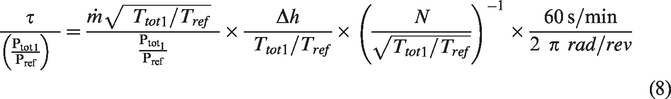
Using this parameter solves the definition issue at sub-idle and, along with pressure ratio and corrected mass flow, has successfully been used5,13 to represent compressor maps down to zero speed. As such, the parameters of corrected mass flow, corrected shaft speed, pressure ratio, and corrected torque are the performance parameters selected here when dealing with sub-idle compressor maps.
Windmill signature for map generation
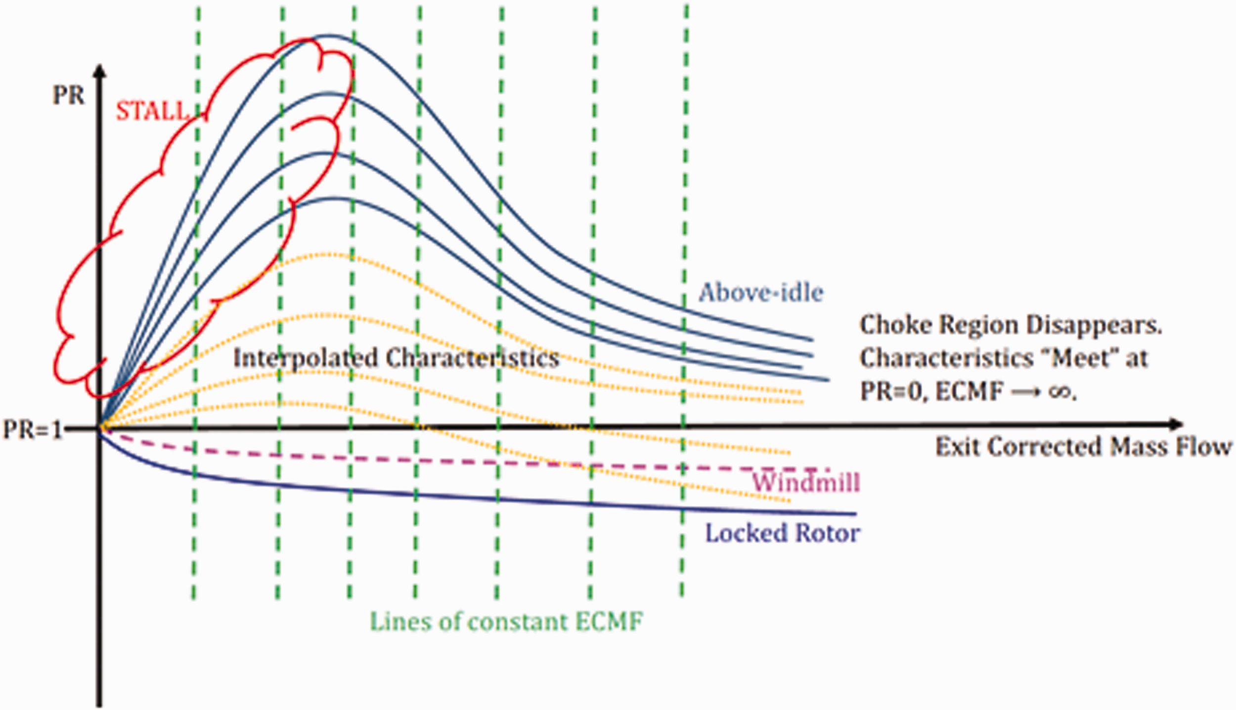
At certain sub-idle speeds, the compressor may be able to impart work on the flow, but aerodynamic losses may be too great for this work to be translated into a pressure rise. A compressor operating in this regime is referred to as a stirrer or paddle, as this is analogous to the physics behind rowing a boat or stirring a beverage. At lower sub-idle speeds and/or pressure ratios, the compressor begins to extract work from the flow, acting like a turbine powered by the incoming flow.18 A locus of points exists on a map dividing the turbine region from the stirrer region. Along this line, the compressor windmills with no net effect on the flow total enthalpy. It must be emphasized that this is a very specific condition in which aerodynamic torques balance out to give no net work addition. A windmilling engine may result in a compressor operating point above or below this “compressor torque-free windmilling line”, depending on the turbine work and the extent of shaft work extraction.19 NACA provides a good early reference on windmilling compressors.20
A linear relationship between windmilling mass flow and speed for the case of fans has been described in the literature.21,22 This relationship was also seen to apply in the case of a multi-stage axial compressor.10 This linear relationship means the windmilling regime can be represented by a single point on a 
Methods to calculate the windmilling mass flow, speed and losses have been created for fans.21,23 This allows the windmill signature to be calculated for a known geometry. These methods are not applicable to multi-stage machines however.
Low speed characteristics corresponding to incompressible flow conditions have been shown to collapse onto a single line.22 With knowledge of the windmill signature, the collapsed low speed characteristic could be interpolated to read the sub-idle portion of the map as shown in Figure 1. Knowledge of the windmill signature yields an anchor on the
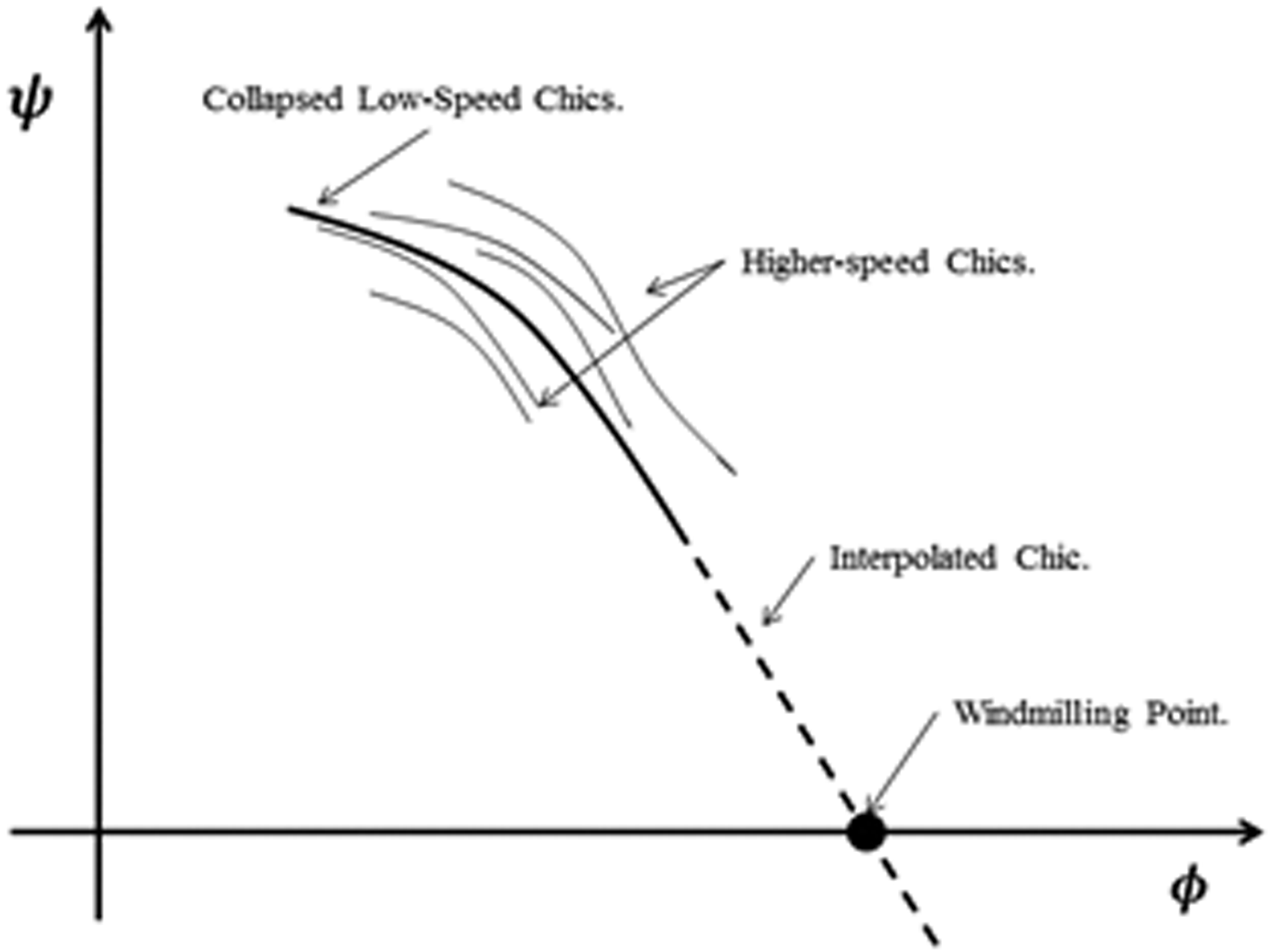
Conceptual use of windmilling point for sub-idle map generation using linearized parameters.
It has been shown10 that maps interpolated solely from the locked rotor line did not accurately capture the windmill points that had been obtained experimentally, pointing to the fact that the interpolation from locked rotor alone does not accurately capture the characteristics near the torque-free windmill line. This can be rationalized from the change in operating regime undergone by a compressor in sub-idle operation, where compression may give way to expansion and where work is ultimately extracted from the flow. An interpolation process that does not make use of this line will have no information on the location of the region where the sign of the work changes. The more calculated characteristics that are included in the interpolation, the more accurate the interpolation will be. The torque-free windmill line provides a physically meaningful choice for an additional characteristic, as it sets the boundary between compressor operating modes. It also ensures more accurate windmill relight performance simulation, as the compressor would be expected to operate near this line (though not exactly on it) when coupled to the rest of the engine. Figure 2 shows how the inclusion of the torque-free windmill line sets the boundaries in operating regions on a map.
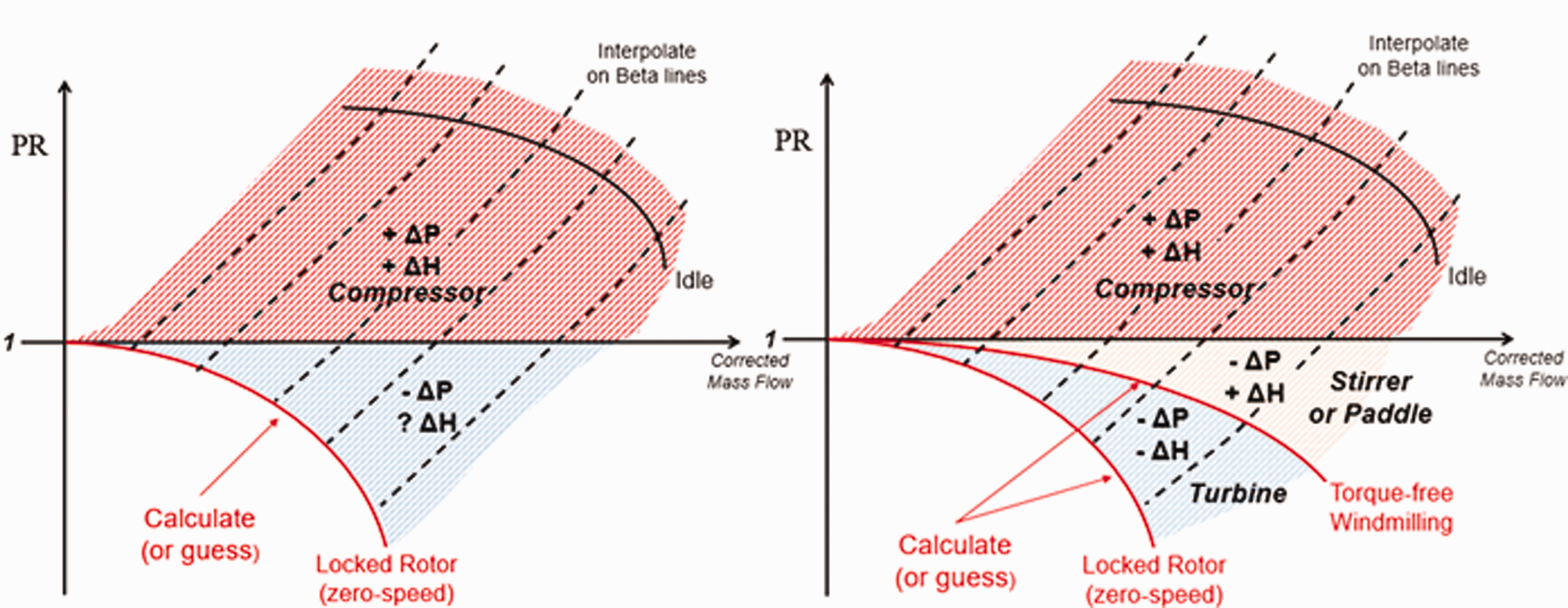
Sub-idle map interpolation without (left) and with (right) the torque-free windmill line.
An additional benefit of using the torque-free windmill line is that, as a non-dimensional point, it can be expected to operate with the same axial flow and loading distribution. This entails that a single blade performance model specifically tuned to handle windmilling conditions can be applied for all points on the torque-free windmill line. In addition, a windmilling compressor can be expected to be dominated by negative incidences, especially in the rear stages, so the same negative incidence correlations used for the locked rotor calculation can also be applied to the torque-free windmilling case.
Map generation method
The method presented here relies on the calculation of two specific sub-idle characteristics: locked rotor and torque-free windmill. This is followed by interpolation up to an existing sub-idle map. It is important to note that an above-idle map is required. This may come from experiment or another existing characteristics calculation tool such as a through-flow code, mean-line analysis or even CFD. The method requires the calculation of locked-rotor and torque-free lines that set the operational boundaries of the sub-idle map. Interpolation between these calculated lines and the above-idle map is then carried out. This serves to further populate the map and assess relevant trends. Aside from the definition of the above-idle map, the method broadly consists of the following three sequential steps:
Calculation of locked rotor and torque-free characteristics, Interpolation Physical Trends Assessment
These steps are described in detail below.
Calculation of locked rotor and torque-free characteristics
The physical accuracy of this map generation method relies on the calculated locked rotor and torque-free characteristics. To do so, this, a mean-line analysis has been employed here. A one-dimensional mean-line analysis provides a simple, robust, and quick approach to generate characteristics from minimal inputs. A mean-line geometry specification may be available during the early stages of engine development. The mean-line approach is well understood and requires little discussion. For a detailed description of the approach, turbomachinery textbooks may be consulted.16,24,25 In summary, the compressor blading geometry at the mean radius is specified in terms of blade metal angles, solidity (chord to pitch ratio), stagger and flow-path radii. For a given flow and RPM, the velocity triangles are solved blade by blade. Calculations are typically carried out in the blade-relative frame, with blade performance correlations used to obtain the total pressure loss and deviation angle expected as a function of blade incidence (difference between the blade-relative inlet metal and flow angles) and geometry (solidity, stagger and blade profile). Work addition and angular momentum conservation due to the mean-radius variation is considered and an iterative solution is used to solve continuity across the blade passage. Bleed and variable geometry can be included in the mean-line calculation. Variable guide vanes can be accommodated by re-staggering the geometry, while bleed is handled by a simple flow deficit which affects the velocity triangles.
The most important aspect determining the accuracy of a mean-line calculation is the set of correlations used for blade performance. These are typically empirical correlations relating blade loss and deviation to blade geometry, and they are usually produced for cases near design incidence. In order to make the mean-line analysis applicable to sub-idle, a loss and deviation model specifically developed for high-negative incidence is required.26 A key assumption made is using this model is that, at high negative incidence, blade-profile losses (in the form of large separated wakes) will be the dominant loss mechanism, so no other loss mechanisms are accounted for. The model has been generated from parametric sweeps of blade profiles with different stagger and solidity settings and a range of negative incidences spanning the sub-idle regime. A single blade profile representative of modern core compressors was used in that work under the assumption that the nature of the separated flows present will result in a minimal impact of blade profile on the loss and deviation characteristics.
In order to calculate the compressor windmill signature as defined in equation (9), a non-linear solver is coupled to the mean-line calculation. The corrected mass-flow that yields zero torque is calculated for a sensible sub-idle RPM, (10% of design speed is used here). This is calculated with a Newton-Raphson method and iterative calls to the mean-line calculation function. The linear windmill flow-to-speed relationship already discussed entails that only one point needs to be solved. The resulting windmill signature then sets the windmill speed associated to a given mass-flow. This allows the entire windmill line to be generated for increasing values of corrected mass-flow until choke is detected in the mean-line calculation. Choking is detected whenever Mach number is beyond unity at any station or when continuity in a blade passage via a density-lagging method can no longer be solved.27 In this method, the mean-line calculation of the locked rotor and torque-free lines is stopped whenever choking is detected. This is not an issue when it comes to interpolating up to choked regions of above-idle characteristics, as the interpolation method devised is able to handle this.
Interpolation
Interpolating characteristics is a useful approach even if accurate characteristic calculation methods exist, as it ensures physically consistent performance data to zero speed. Compressor design establishments seeking to obtain sub-idle compressor maps will typically have established methods for generating compressor performance data above idle. This data may come from rig tests, scaling of previous designs, or validated numerical codes with a number of empirical corrections ensuring adequate alignment with measured data. In any case, there will be a high degree of confidence in the above-idle data obtained with these methods, while no such data will be available below idle.
While an analytical method could be developed to accurately calculate all sub-idle characteristics, there is no guarantee that these will match seamlessly with existing above-idle data generated with the “high confidence” methods. This can lead to a discontinuity in the region where both sets of data meet. Thus, in developing a method that can be used to quickly generate sub-idle characteristics from a limited set of inputs, it becomes imperative that the method yields a set of performance data that seamlessly matches existing above-idle characteristics. This avoids unphysical discontinuities from the “stitching together” of datasets from different sources. An example of this can be seen in Figure 3, where a mean-line method is used to generate sub-idle characteristics all the way up to idle and compared to the result of interpolation from the calculated and pre-existing data. As can be seen, the interpolated characteristics match reasonably well against the calculated ones, with the matching becoming poorer as speed increases. Eventually, the method fails to match the measured above-idle characteristic, since it has not been tailored for calculation in that region. Since compressor design establishments will already have validated methods in the above-idle region, the seamless matching of above-idle and sub-idle data becomes a convenient method for extending these methods down to zero speed.
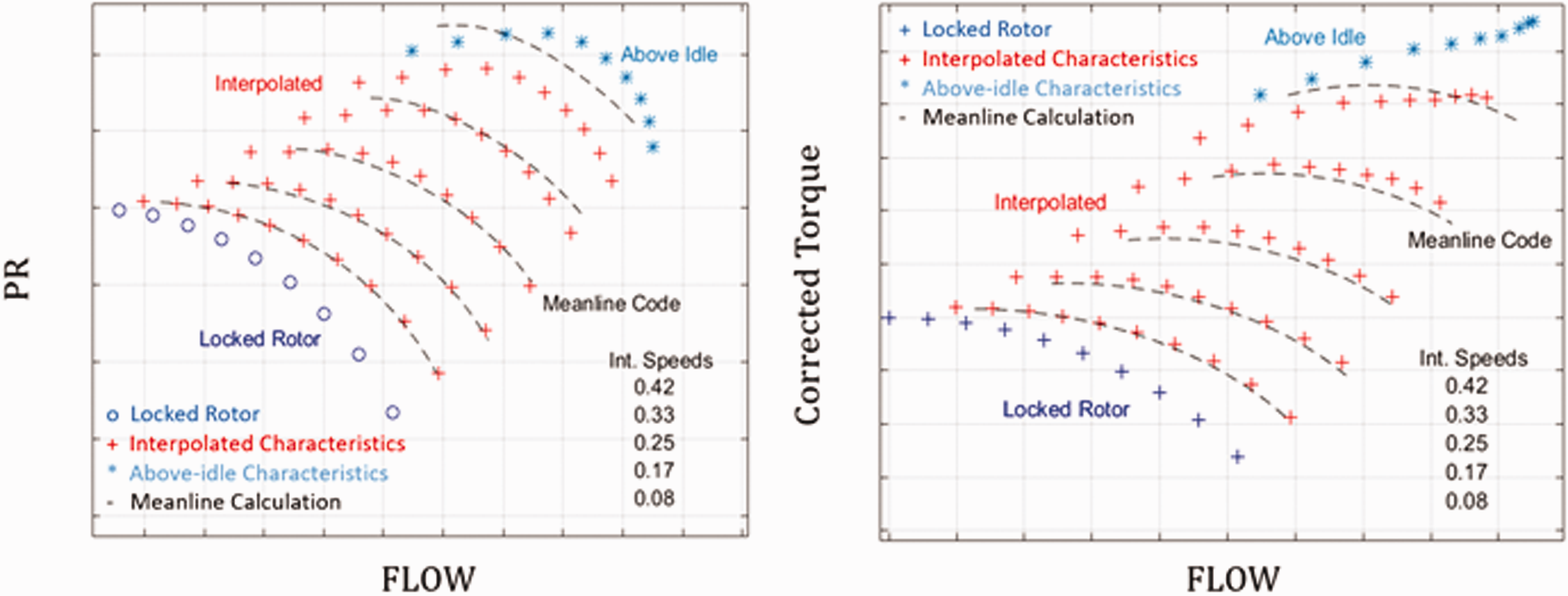
Sub-idle map interpolation and mean-line calculation. PR (left) and corrected torque (right).
Definition of interpolation coordinates
In order to interpolate maps between calculated sub-idle and existing above-idle data, a set of coordinates needs to be defined along which said interpolation can take place. Compressor maps are typically tabulated with the aid of beta lines (also known as R-lines). These lines are devoid of meaning and used simply as an extra coordinate that can be used to set the data in tabular form.28 Previous map interpolation and extrapolation methods have used these beta lines as the natural coordinates along which to carry out interpolation.5,9 This however adds an additional handle to the process: the distribution of said beta lines on the sub-idle characteristics. This may become particular problematic in the choking region, where no guidelines exists as to how these should be arranged along a vertical characteristic to ensure smooth interpolation. In order to avoid these limitations, the use of exit corrected mass flow is proposed here as a method for tying together performance at different speeds, allowing interpolation to be carried out along unambiguously defined physical coordinates.
Figure 4 shows how a compressor pressure ratio map may look after converting the mass flow coordinate to an exit corrected mass flow (ECMF) which may be defined as:
Sub-idle PR map using exit corrected mass flow (ECMF).
With the standard compressor map, exit stagnation conditions can be obtained and the ECMF calculated for each point. This allows the blue above-idle lines in Figure 4 to be obtained directly from the existing data. Calculating the ECMF for the calculated locked rotor and torque-free windmill lines allows these to be added to the plot as well. Using ECMF immediately eliminates one of the issues associated with map interpolation: the ambiguous definition of characteristics in the choke region. While characteristics may have a constant inlet corrected mass flow when choked, they will have different ECMF values due to the drop in pressure and efficiency as the operating point moves down the choked characteristics. Via ECMF, this difficulty is removed as points on the choked regions of different characteristics can be tied together via a constant value of ECMF. If interpolation is required in the choking region but one of the characteristics does not extend sufficiently into choking, it can easily be extrapolated to larger ECMF as seen in Figure 4, allowing interpolation to be carried out. An issue remains however, and that is the lack of data in the stall region of the map for the above-idle characteristics. After plotting with ECMF, the above idle characteristics can be fitted with a smoothing spline that joins the peak pressure (or lowest ECMF points) with the PR of unity point at zero ECMF, establishing this as a limit value. This then provides at least a mathematically consistent way of establishing the coordinates along which interpolation will take place in this area of the map. The resulting interpolated characteristics may then be “chopped” in the stall region in accordance with a consistent stability line definition (such as peak PR) or by a more sophisticated method for determining the stall drop-in point.29,30 Figure 4 shows the stall region of the map where the use of this smoothing spline may be required to join peak pressure points to the zero flow condition.
Interpolation along lines of constant ECMF may be carried out using any preferred mathematical function. The piecewise-cubic hermite interpolating polynomial (PCHIP) is preferred by the authors, as it results in smooth functions without the overshoots that can be obtained from spline interpolation. The justification for a smooth trend being desired along the lines of constant ECMF comes from their definition, as we may consider operation along a line of constant ECMF to be equivalent to operation along a throttle line, where a downstream device keeps the outlet flow function constant. It is important to note that for subsonic cases, beta lines may be defined in terms of constant work coefficient, allowing unambiguous physical interpolation coordinates to be defined. This however breaks down in the choking region, where the subsonic assumption does not apply.28 The use of ECMF eliminates this issue. The notion of constant ECMF is somewhat similar to the Exit Guide Vane Mach number used by Kurzke15 to set the locked rotor choking point, although it is not used there as a means to define physical interpolation coordinates.
Physical trends assessment
After a map has been generated, it is important to check that the generated sub-idle characteristics obey expected physical trends. Replotting the generated sub-idle characteristics using flow and work coefficient as defined in equations (5) to (7) allows for a first order check on the physicality of the outcome. It is important to note that the locked rotor line cannot be defined in terms of these parameters, however. By plotting the characteristics in terms of these linearized parameters, we can test whether the interpolated characteristics collapse at low speed, and whether all characteristics follow a smooth trend with negative slope. All characteristics are “anchored” by the torque-free windmill point, as they must all cross the zero work coefficient point at the same flow coefficient. If this results in a kink, the windmill signature calculated does not align properly with the rest of the data and could be considered to be in error.
Due to the simplified model involving a one-dimensional mean-line analysis, the windmill signature calculation can potentially be in error, so the windmill signature as defined in equation (9) may need be adjusted manually until the expected trend results. This is the only user handle available in the method, and is required only to allow for the mitigation of the limitations inherent in the mean-line analysis. Figure 5 shows an adequate linearized parameter trend as well as two other trends that may be associated to different issues with the generated maps. Figure 5(b) shows a trend that may require adjustment of the windmill signature. Figure 5(c) shows a typical plot that results when the torque-free windmill is not used, where the low speed characteristics fail to collapse unto a single line as predicted by theory.21,22
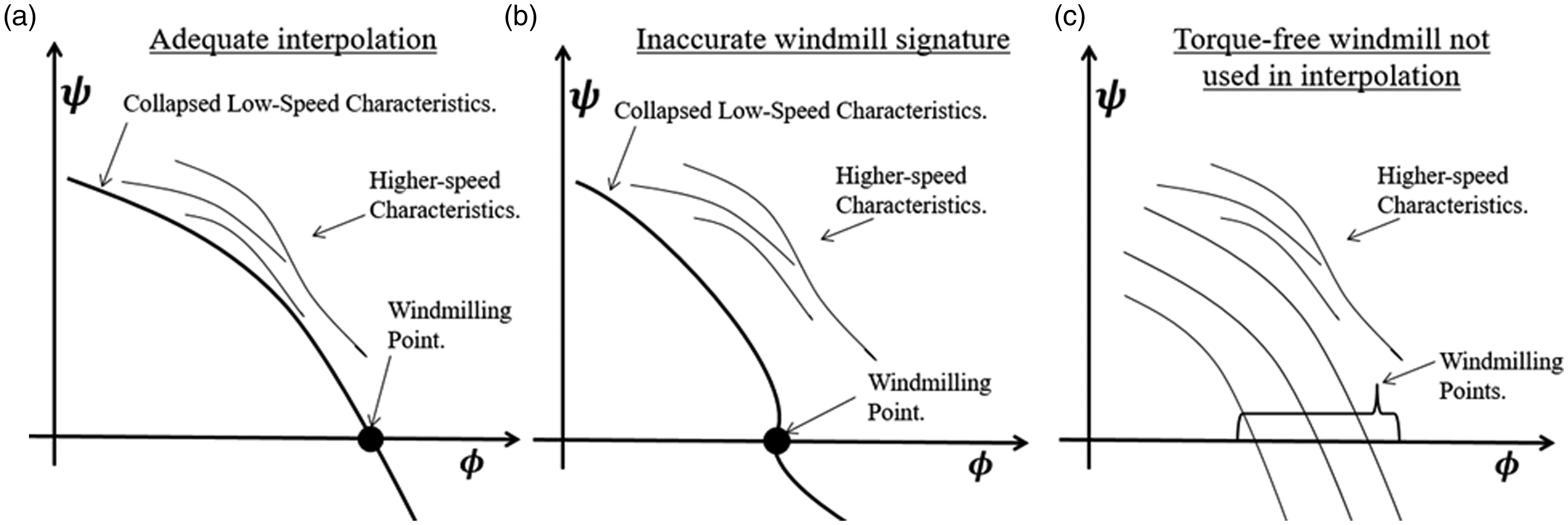
Adequate linearized map (a) and two possible issues with interpolation (b,c).
It is worthwhile to note that in the absence of any geometry data, a guess of locked rotor choking flow can be made and a locked rotor line drawn based on a quadratic loss curve. The linearized characteristics can then be used as in Figure 5 to guess an appropriate value of windmill signature, which can then be used to set a torque-free windmill line from which to interpolate. This approach can be combined with methods in15 when absolutely no geometry data is available.
Map generation method summary
The overall methodology may be enumerated in detail as follows:
Specify mean-line geometry & above-idle map. Calculate locked rotor (RPM=0) characteristic using mean-line analysis. Use a Newton-Raphson method which executes a mean-line analysis at a single specified RPM until the mass flow that yields zero torque is found. This specifies the windmill signature as defined in equation (9). Calculate the torque-free windmill line via mean-line analysis. Knowledge of the windmill signature allows us to specify the torque-free RPM at each mass flow. Re-sample the calculated characteristics at values of exit corrected mass flow (ECMF) that match those of the points to be used for interpolation on the lowest above-idle speed. Interpolate along lines of constant ECMF using PCHIP or desired interpolation function. Plot the linearized characteristics (work vs. flow coefficient) and check that they follow the expected linear trend at low speed, with low-speed characteristics collapsing unto each other. Ensure the low-speed characteristics pass through the same point at null work coefficient and that this does not introduce a “kink”. Otherwise the windmill signature may need to be adjusted. Resample the characteristics as required for loading into performance model.
Sensitivity study method
The previous section has detailed a new method to generate compressor maps to zero speed. What follows is not part of the map generation method. This section instead describes a method used in a sensitivity study performed to understand the impact that map inaccuracies may have on performance models. This study seeks to provide guidance as to the accuracy required in sub-idle maps. Many of the map generation methods available in the literature rely on approximations and, at times, crude assumptions. While this may be warranted due to lack of data, proper consideration must be given to the impact that these inaccuracies may have in performance calculations. Such a study is not available in the literature, and the outcomes help justify the reasoning behind some of the methods employed in the map generation process.
To perform this study, a core-flow compressor model was developed. The model is a compressor matching scheme that iterates to find the operating point on a compressor map. Only the core compressor is considered in the model, without regard for any of the other engine components. Time histories of compressor discharge properties along with inlet dynamic pressure are inputs, while the compressor flow and inlet properties are model outputs. Models like this can be used to indirectly determine core flow from reliable temperature and pressure measurements in an instrumented engine. Such an approach requiring compressor inlet and outlet data is used here to allow the accuracy of the compressor maps to be evaluated against measured data from ground-start tests performed on a real aero engine. This compressor-only matching scheme eliminates the confounding effects that may arise from using a whole-engine model. This allows us to evaluate the accuracy of the compressor maps, as the effects of other component characteristics are removed.
While mass flow measurements taken during whole engine sub-idle testing with sensors calibrated for nominal conditions may be prone to error, total pressure and temperature readings from such tests are considered more stable. If a dynamic or static pressure measurement at the compressor inlet is available, this may be used along with the outlet total pressure, total temperature, and shaft speed to calculate the rest of the inlet properties, including mass-flow, using compressor maps. It is important to note that the measured data that is available may depend on the engine test, so that different available data sets may yield different model setups (with different inputs and outputs). The model inputs and outputs used here correspond to the data that was available in this specific case. The key aspect is not the model setup itself, but how some limited test data can be used to test the compressor characteristics independently of a whole-engine model.
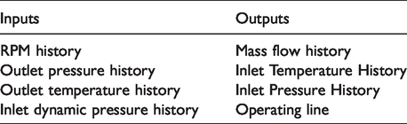
The model consists of two nested non-linear solvers. The first solver tries to solve for the mass flow into the compressor by varying the inlet temperature. With the value of inlet temperature known, the corrected speed can be set. The second solver can then iterate at the known corrected speed to find the beta-line that matches the enthalpy change through the compressor. With knowledge of this beta-line, the pressure ratio map can be consulted and used to calculate the inlet total pressure from the known outlet pressure. This allows the inlet corrected mass flow to be calculated with knowledge of the inlet dynamic pressure. If the calculated corrected mass flow matches that from the map at the given beta-line, the solution stops, otherwise the top-level solver changes the guessed inlet total temperature and the iterative solution continues. A schematic of this process is shown in Figure 6. The model’s input and outputs are listed in Table 2.
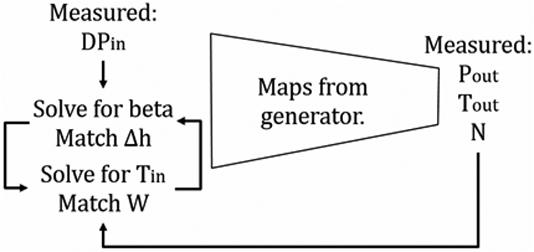
Compressor matching scheme.
Compressor matching scheme inputs and outputs.
It must be emphasized that this model is used here not as a compressor analysis tool, but simply as a method for testing the map’s performance. Artificial time histories may be used as inputs solely to ensure the calculated operating lines follow expect trends, with no undesired jumps or kinks due to crudely interpolated maps. Likewise, the sensitivity of performance transients to changes in the sub-idle characteristics can be assessed by employing the same input data with the different characteristics and comparing the resulting transients.
Using this compressor matching tool, the sensitivity of performance calculations to changes in the sub-idle map can be assessed by altering the underlying locked rotor and torque-free windmill characteristics as well as the windmill signature by a pre-set amount. In this work, the locked rotor and torque-free windmill lines have been scaled up and down by 30% as shown in Figure 7 to assess the effect this has on the calculated transients obtained from the compressor matching scheme.
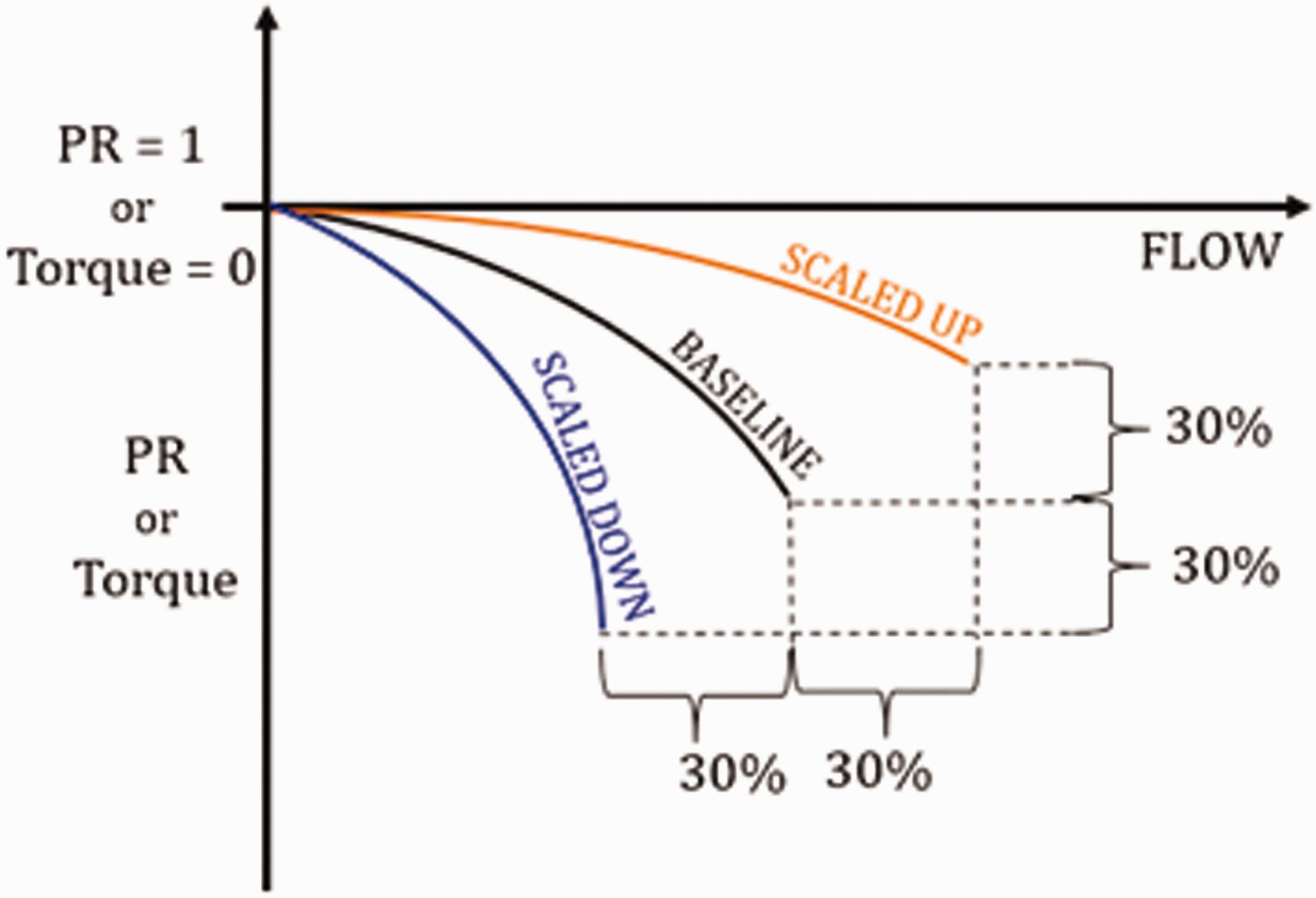
Characteristic scaling for sensitivity study.
Results
Results of the mean-line analysis for the calculation of locked rotor and torque-free windmill characteristics are first discussed. The sensitivity of the sub-idle maps to these characteristics are then investigated. Later, the effect of the inclusion of the torque-free windmill line and the importance of the beta-line specification are assessed.
Mean-line calculation accuracy
The accuracy of the mean-line calculation employing the negative incidence correlations27 is assessed by comparing against numerical data obtained from 3 D RANS CFD of 4 different multistage compressors named: M250, MCCA, MCCB, and MCCC. The M250 is the six stage axial component of the Rolls-Royce Allison Model 250 compressor. The other three compressor geometries correspond to core compressors from modern aero-engines. While the M250 has moderately low hub to tip ratios (∼ 0.4) the other geometries have representative hub to tip ratios in the 0.7-0.8 range. These geometries have been selected because they represent typical core compressor geometries currently in use in modern aero engines. Figures 8 to 11 compare the locked rotor (zero speed) and torque-free windmilling characteristics calculated. Torque values have been normalized by a nominal operation value. The MCCB has a higher stage count than MCCA and MCCC, resulting in a different range of normalized torque. It is important to emphasize that the torque-free line does not occur at single speed, as it ties all points for which torque is null at different speeds. The locked rotor characteristic is represented by pressure ratio and torque vs. mass flow, while the torque-free windmill characteristic is represented by pressure ratio and windmilling shaft speed vs mass flow. All characteristics are calculated up to choking using the mean-line code. For the case of the M250 in Figure 8, experimental data obtained from a rig10 can also be plotted, but this does not encompass the entire range of the characteristic up to choke.
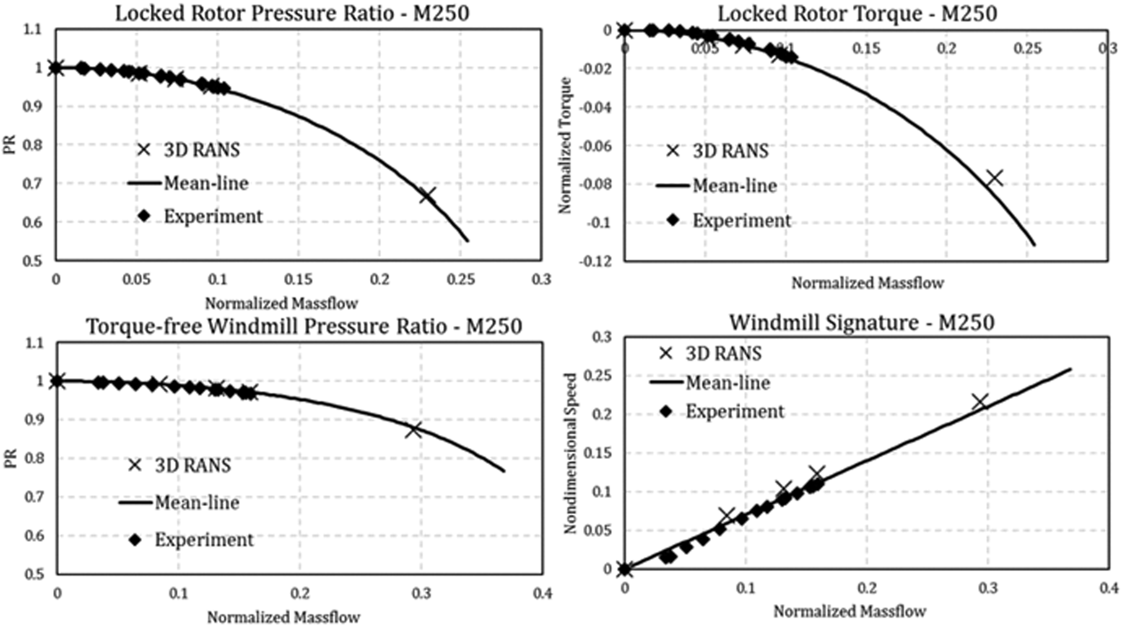
Mean-line calculation for locked rotor and torque-free windmill for M250. Comparison against CFD and experiment.
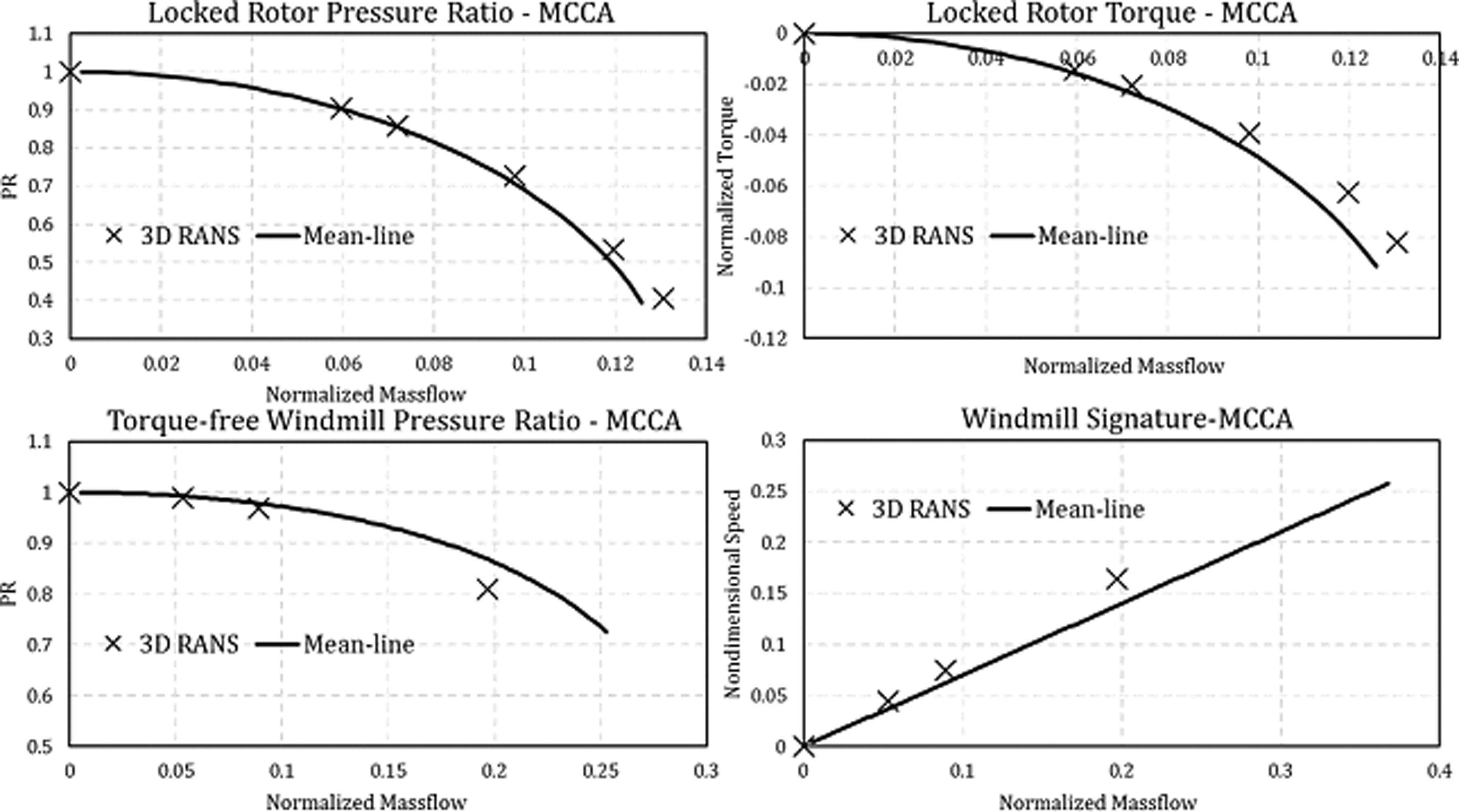
Mean-line calculation for locked rotor and torque-free windmill for MCCA. Comparison against CFD.
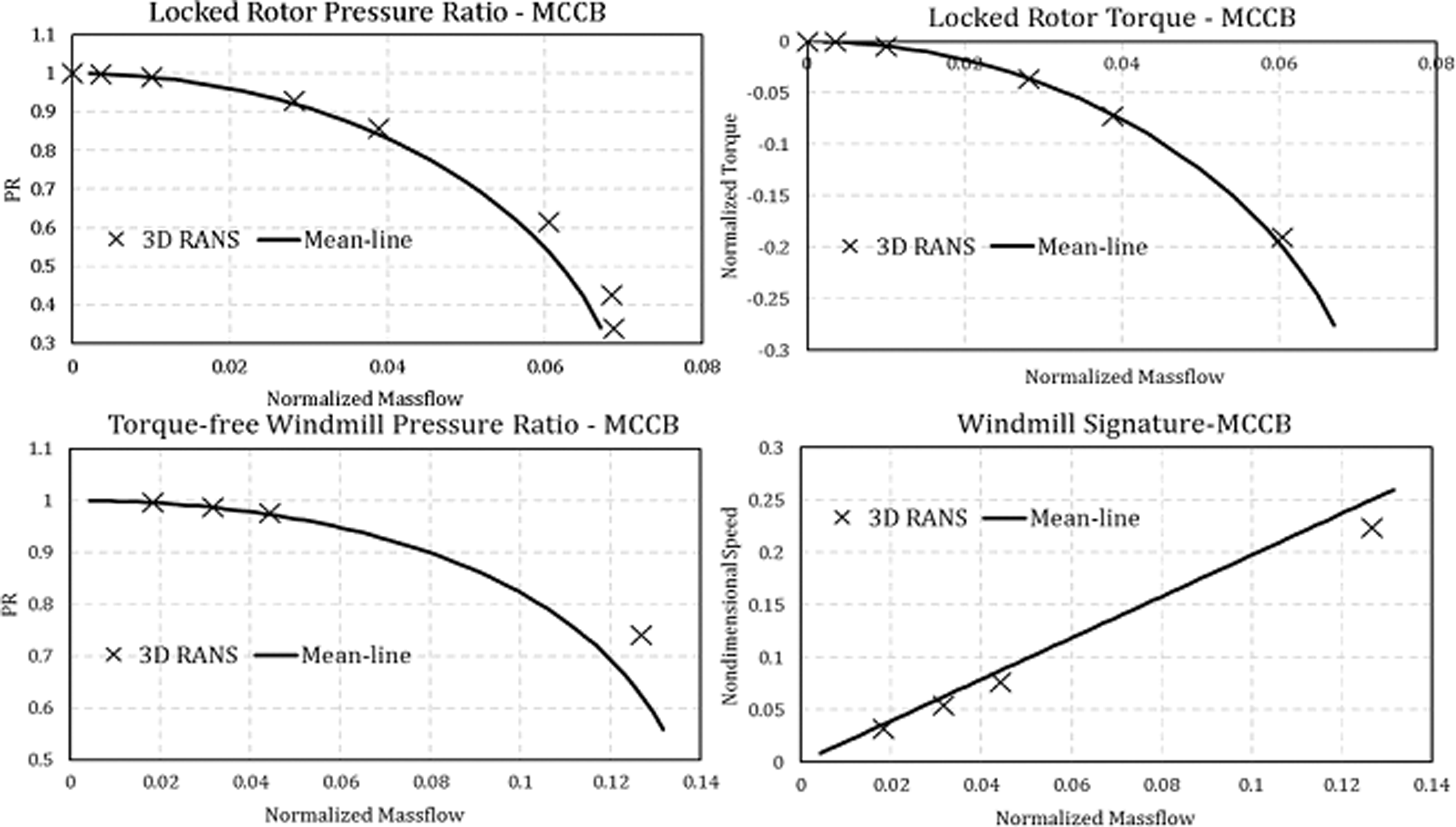
Mean-line calculation for locked rotor and torque-free windmill for MCCB. Comparison against CFD.
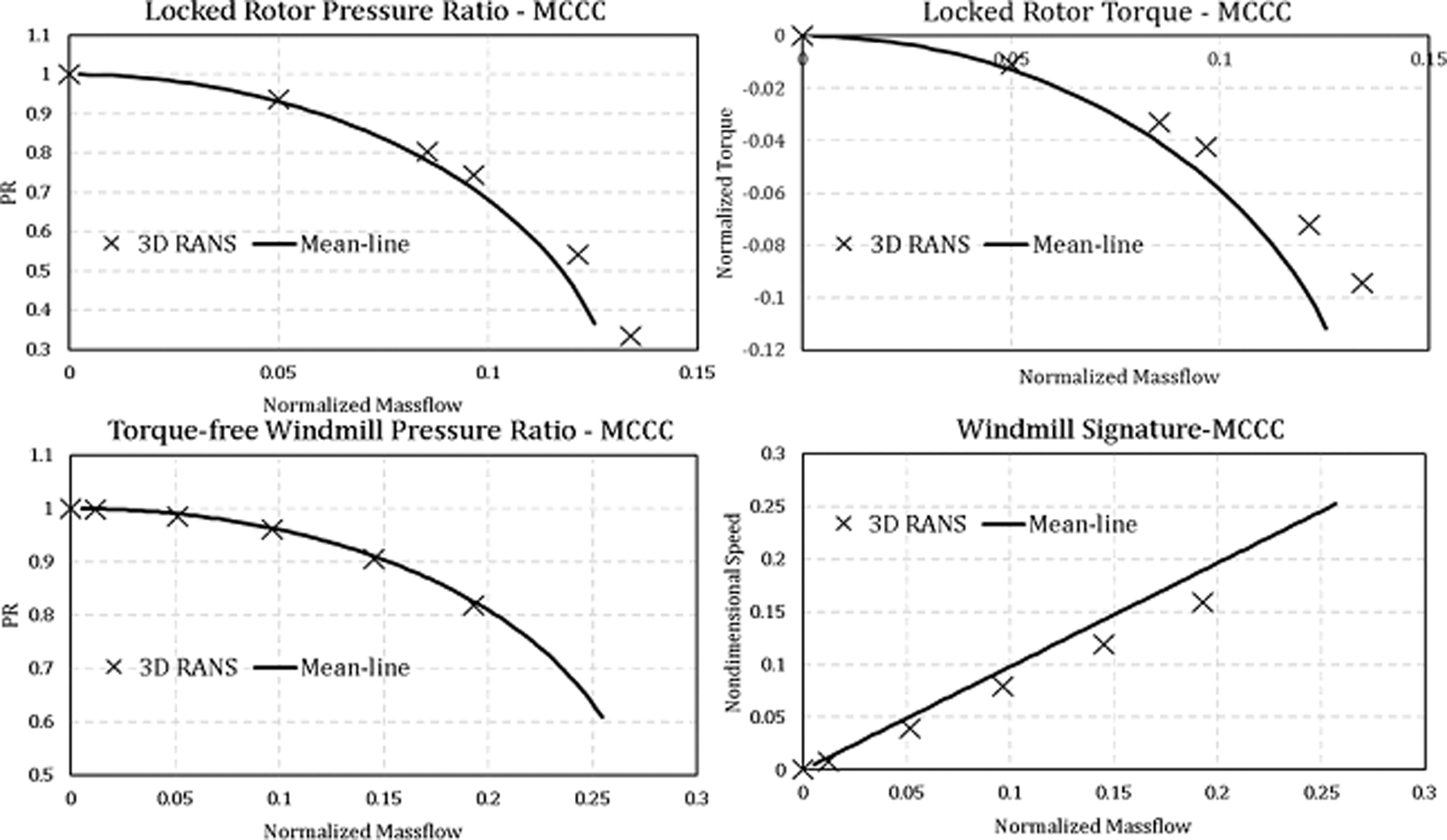
Mean-line calculation for locked rotor and torque-free windmill for MCCC. Comparison against CFD.
Judging from the matching in Figures 8 to 11, the mean-line analysis can generally be considered to provide outputs equivalent to CFD results. Considering the instantaneous execution time (<0.1 s) of the mean-line analysis compared to the much more costly 3 D RANS CFD, the mean-line approach seems to be the adequate way forward for characteristics generation, especially when input requirements are considered. In all cases, and more so in the case of the MCCC (Figure 11), the mean-line analysis and CFD begin to diverge as the choking point is reached, especially with regards to the torque characteristic. This may be reasoned from the 1 D nature of the mean-line analysis, where choking is reached abruptly, rather than the gradual choking and mass-flow redistribution that would be captured by a through-flow or 3 D analysis. For the MCCC geometry shown in Figure 11, the difference in flow between mean-line and CFD at −0.1 Normalized Torque on the locked rotor line is 10%. This is the largest mismatch observed in all three geometries. It is important to note that while percentage errors may appear large, the torque values for these compressors at locked rotor are small compared to nominal operation, so that apparently large relative errors translate to moderate mismatch in absolute terms. There is a level of uncertainty in torque values obtained from steady state RANS CFD of multistage compressors operating at these conditions. In the study presented in,31 uncertainties for torque values obtained from CFD of locked rotor compressors were reported as ∼5%. This study has used the same methodology detailed in that work. Considering these limitations, the error between mean-line analysis and CFD for the MCCC geometry may be considered less significant. Furthermore, the MCCC is the newest geometry of those investigated, so that 3 D design effects in the blading not captured by the 1 D mean-line approach may be behind the comparatively larger discrepancy. As shall be seen, these discrepancies near choke have little impact in the generated maps and resulting performance calculation.
Sensitivity to mean-line results
As highlighted above, while the mean-line analysis appears to be a powerful tool for the purposes of this work, confidence in the accuracy of its results at high mass flows diminishes in light of the difference when compared to 3 D CFD near the choking mass flow. This may be a small limitation, however, when the nature of sub-idle operation is considered. A compressor will operate along the locked rotor line only when flow is passed through it by some other means, such as when it is not the powered compressor during a cranked start or when it is locked mechanically in flight. In these cases, it is unlikely that its operating point will be pushed anywhere near the choking mass flow. Ground started un-cranked compressors will quickly accelerate close to the stability margin, while the high bypass ratios experienced during an inflight flameout would limit core flow during locked rotor operation in flight. However, the effect that inaccurate near choke locked rotor regions can have on the rest of interpolated characteristic needs to be considered. This can be addressed via a sensitivity analysis using the compressor matching scheme previously described.
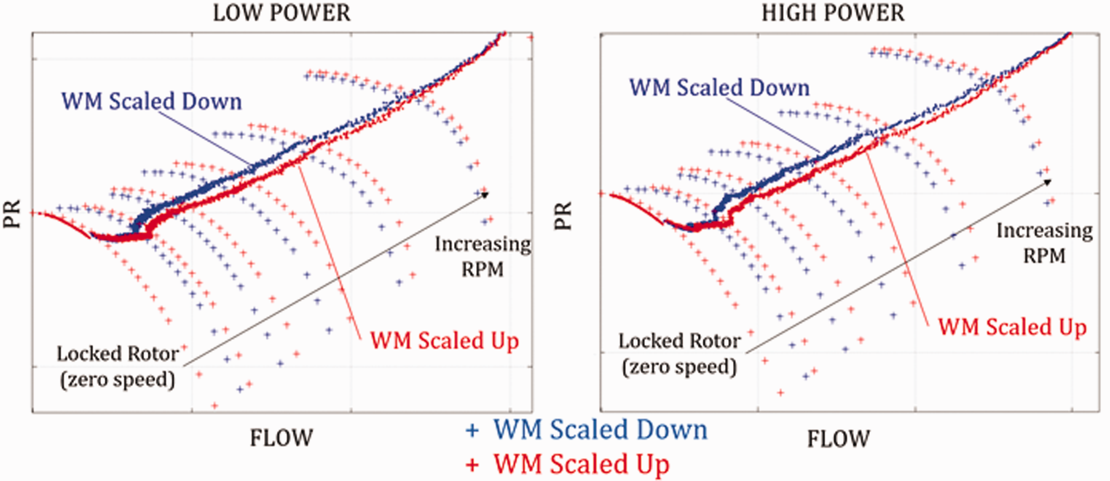
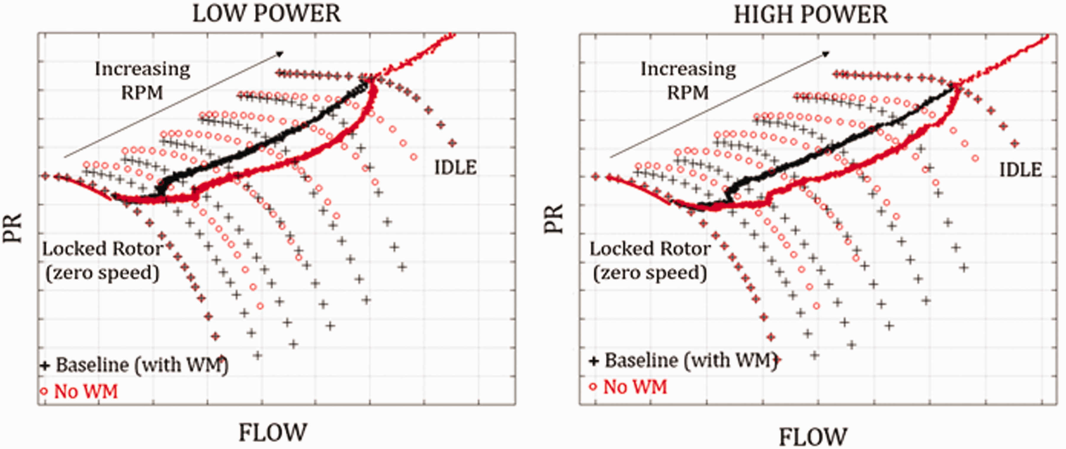
Figure 12 shows the calculated ground start transients for two different ground start cases termed low and high power, due to the different power settings used on the starter motor. The high power case uses nominally twice the starter power than the low power case, but it is important to note that another core compressor in this multi-spool engine architecture is connected to the starter. The compressor investigated here is not cranked during the ground start, hence its initial operation along the locked rotor line. Real experimental test data is used to set the compressor outlet conditions per Table 1. Two different maps are used in each case, where the locked rotor line (in terms of both PR and torque) has been scaled respectively up and down by 30% as illustrated in Figure 7. The effect of the change in the locked rotor choking region is drastic in the high mass flow area of the map at very low speeds, but quickly loses its impact at high speeds. Since the operating line stays closer to the stability line, these changes on the calculated map do not greatly affect the calculated transient.
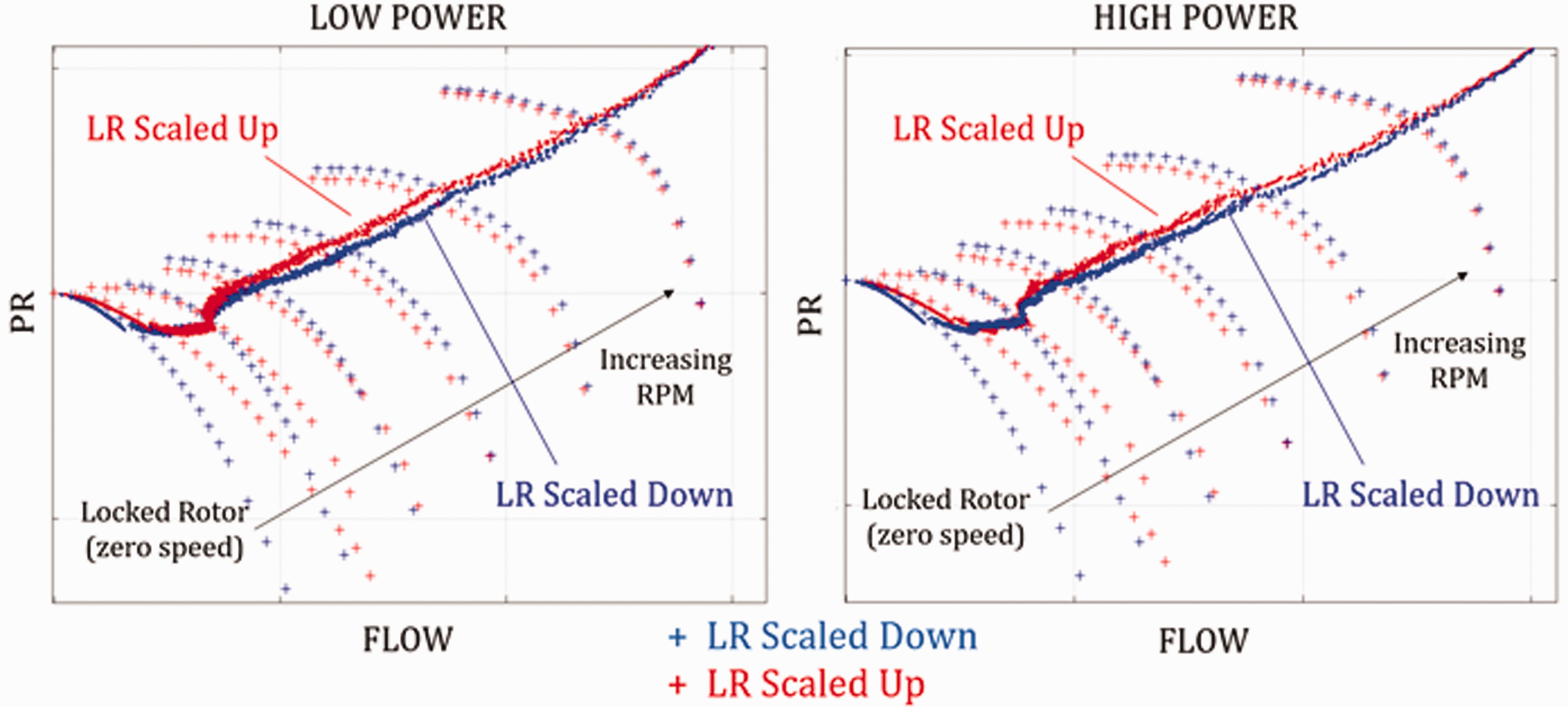
Sensitivity of performance prediction to locked rotor line calculation for low (left) and high (right) power starts.
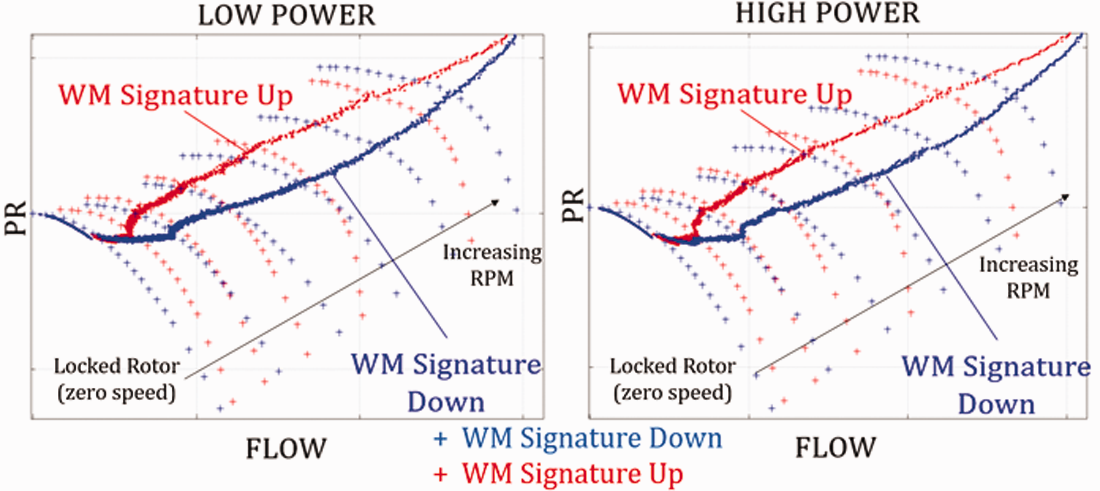
Similarly to Figure 12, Figure 13 shows a similar study for the case where the torque-free windmill pressure ratio characteristic is scaled up and down according to Figure 7. In this case, we see the effect is more pervasive into higher speed characteristics, however the effect on the calculated operating line is still quite limited.
Sensitivity of performance prediction to torque-free windmill line calculation for low (left) and high (right) power starts.
In order to calculate the torque-windmill line, a mean-line analysis together with a Newton-Raphson solver is used to calculate the windmill signature as defined in equation (9). This allows the windmilling mass flow and speeds to be tied together so mean-line analysis can be applied along the torque-free windmill line. Inaccuracies in the windmill signature calculation can give rise to different maps due to its impact on the interpolation. This is seen in Figure 14, where the calculated windmill signature has been scaled up and down by 30%. This yields noticeably different maps with very noticeable changes in the calculated transient operating line that results. From these results in Figures 12 to 14, it becomes clear that the accuracy of the locked rotor choking region is of little importance in the map generation, however the calculation of an accurate windmill signature is much more relevant.
Sensitivity of performance prediction to windmill signature calculation for low (left) and high (right) power starts.
Effect of windmill signature and beta-line definition
The previous section has highlighted the effect that an inaccurate windmill signature can have on the calculated maps. It is important thus to assess what effect including a torque-free windmill line in the interpolation has in the first place. Figures 15 to 16 show an interpolated sub-idle characteristic at 15% of design speed, with and without the torque-free windmill line (WM) included in the interpolation. In these figures, 3 D RANS results of the same characteristics are included for comparison. It can be seen that for the two geometries tested, M250 and MCCA, the addition of the torque-free windmill line results in a closer match to CFD. In addition, the interpolated characteristics using the torque-free windmill signature appear much smoother, with no un-physical kinks. This can be attributed to the lack of a “middle anchor” in the interpolation, as provided in the case with the torque-free windmill line.
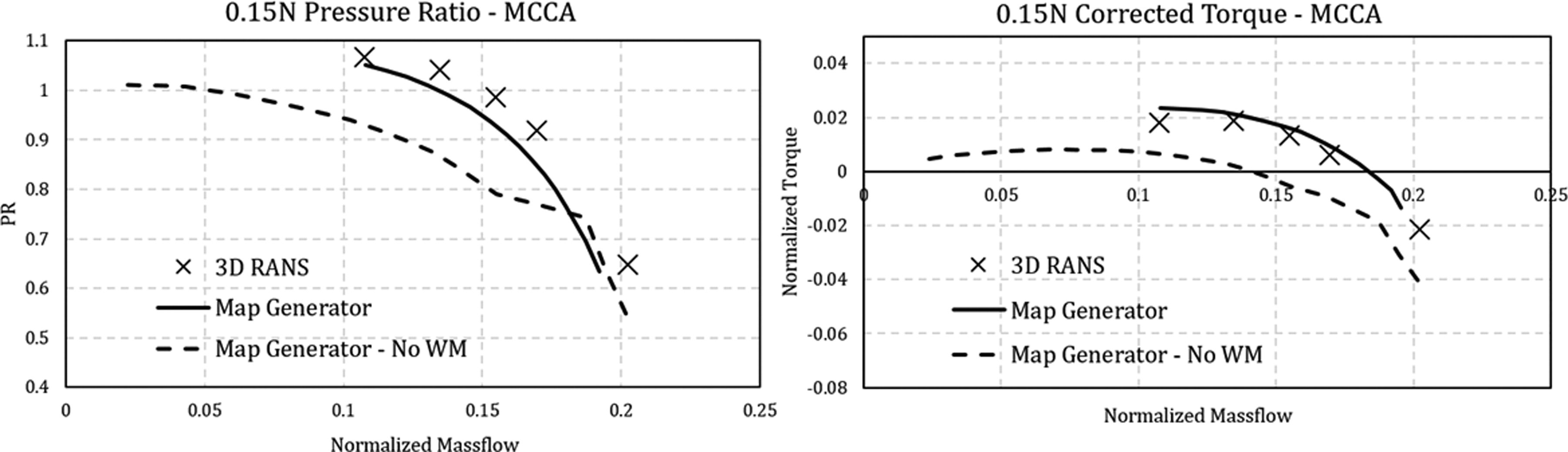
Generated 15% speed characteristic with and without windmill signature and comparison against CFD for M250 geometry. PR (left) and normalized torque (right).
Generated 15% speed characteristic with and without windmill signature and comparison against CFD for MCCA geometry. PR (left) and normalized torque (right).
Interpolating directly between the shape of the locked rotor and the lowest available speed line (without the torque-free line) can result in somewhat unphysical characteristics as the shape transitions from one to the other. These un-physical kinks could be smoothed out through manipulation of the lines used for interpolation, but in that case the manipulation would depend purely on judgement. The use of the torque-free line mitigates this.
Similarly to what was done in the previous section, we use the compressor matching scheme with the same two ground start test cases to assess the effect that the omission of the torque-free windmill line can have on a calculated ground-start transient. As can be seen in Figure 17, the transient operating line that results is greatly affected by the lack of the torque-free windmill line. It may also be said that the black operating line, calculated with maps using the torque-free windmilling line, appears more physical, as it transitions more smoothly into the operating line spanning the above-idle region of the map. Both operating lines converge in the above-idle region as the characteristics are the same there.
Sensitivity of performance prediction to maps with and without torque-free windmill line for low (left) and high (right) power starts.
The definition of physics-based interpolation coordinates in terms of lines of constant ECMF was identified previously as an important addition to the map generation process, as it avoids ambiguity in their definition which could result in inconsistent, or differently-interpolated maps, even when starting from the same set of data. In Figure 18, we show the operating lines that result from maps that have been generated with two slightly different definitions of the interpolation coordinates (beta lines) but identical above-idle map, locked rotor and torque-free windmill lines. While these coordinates may be chosen such that smooth, physically looking maps result, we see that a non-negligible difference arises between the two, even when smooth maps are obtained. Ensuring consistent, unambiguous results when generating the maps is important when working in design environments, justifying the need to define lines of constant ECMF as the coordinates along which to carry out the interpolation.
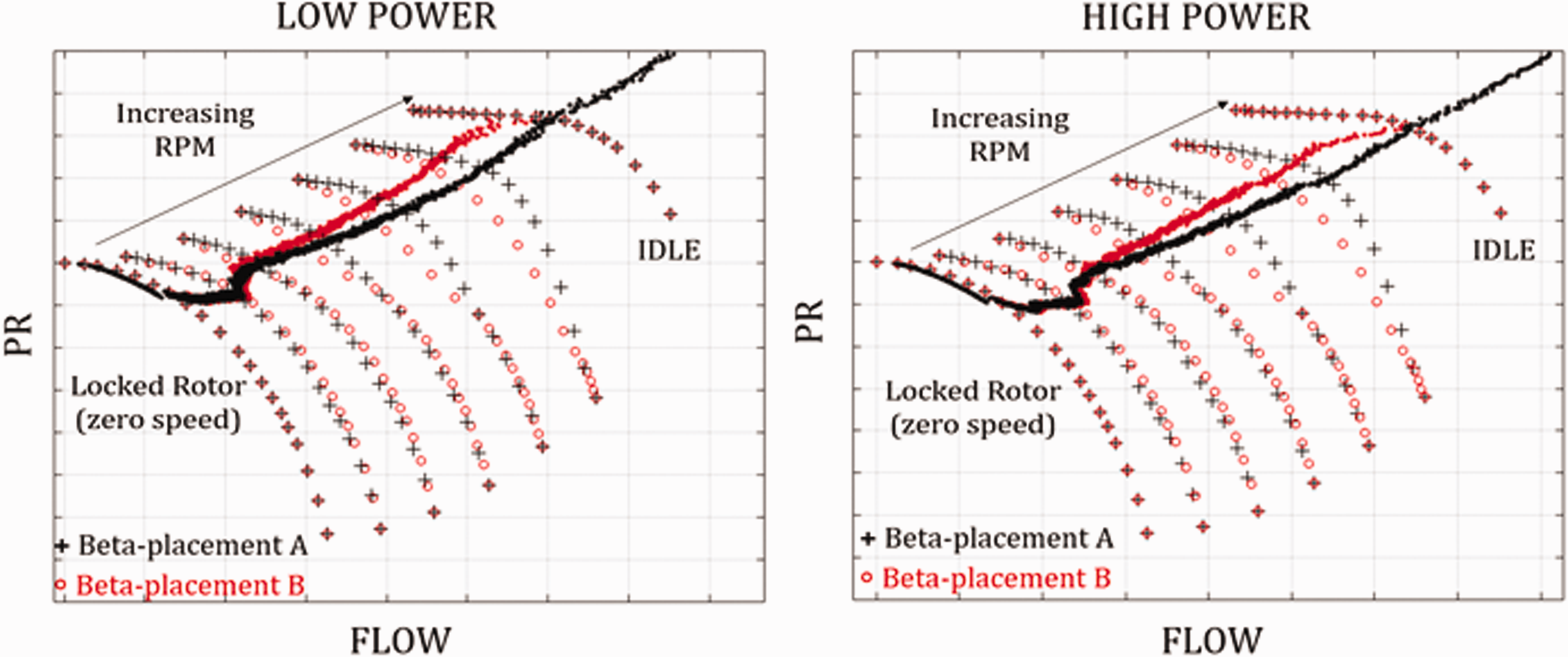
Sensitivity of performance prediction to minute changes in beta lines used for interpolation for low (left) and high (right) power starts.
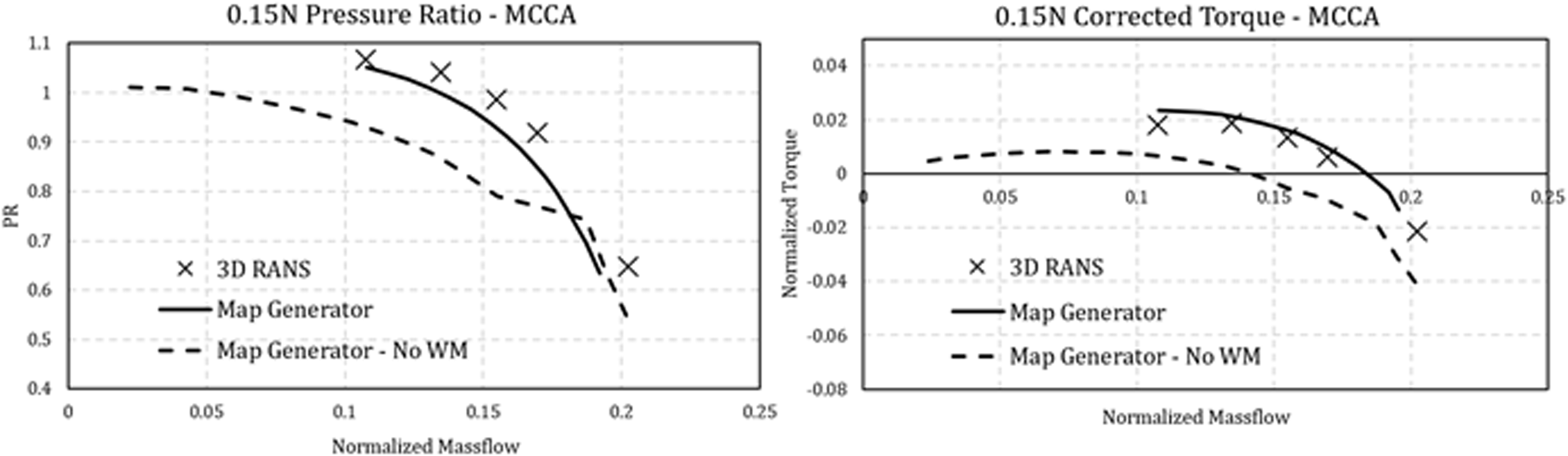
Interpolated map vs. CFD
As a holistic assessment of the map generation method’s merit, we compare the interpolated map that results for the MCCC geometry against characteristics obtained from 3 D RANS CFD. This is shown in Figure 19. While some differences exist, we see the characteristics largely match well. It is important to note that the MCCC was chosen for the comparison as this geometry showed the worst matching between CFD and mean-line analyses for the locked rotor and torque-free windmill line calculated as shown in Figure 11.
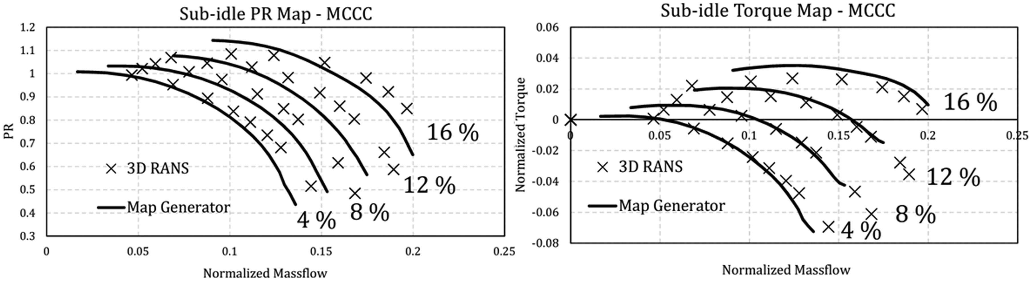
Generated MCCC sub-idle maps vs. CFD. PR (top) and normalized torque (bottom).
Conclusion
A method for the generation of consistent sub-idle maps to zero speed has been identified. The key differences between this and previous methods is the definition of the torque-free windmill line and the use of physically significant interpolation coordinates in place of auxiliary beta lines. The method relies on a mean-line analysis using high negative incidence correlations identified in the literature to calculate the locked rotor and torque-free windmill lines. A Newton-Raphson solver is used to calculate the windmill signature, which ties together the rotor speed and mass flow that yields zero torque. This is then used with the mean-line analysis to obtain the entire torque-free line. The rest of the sub-idle characteristics are interpolated between the results of the mean-line analysis and existing above idle data. The interpolation is carried out along physical coordinates defined as the locus of constant exit corrected mass flow on each characteristic. A piece-wise cubic hermite interpolating polynomial (PCHIP) is used for interpolation.
Comparison against 3 D RANS CFD shows overall good matching of the mean-line analysis. Sensitivity studies show that possible inaccuracies in the locked rotor mean-line calculation, especially near choke, have relatively minor impact on the final map. Calculating a correct windmill signature however, which defines the boundary between stirrer and turbine operation in the compressor, is seen to be much more important. Overall, a good method for the quick extension of existing maps to zero speed has been identified provided mean-line geometry is known. The mean-line line analysis used here is a 1 D approach which can adequately represent high hub-to-tip ratio geometries such as a core compressors. Application to low hub-to-tip ratio geometries such as fans has not been assessed. Higher order methods may be used provided full geometry definitions are available, but the method described here may be used where quick results are required or where full geometry definitions are not yet available (such as in early design stages where scaled maps are being extended to zero speed).
Footnotes
Acknowledgments
The authors would like to thank Rolls-Royce plc. for supporting this work and allowing its publication.
Declaration of Conflicting Interests
The author(s) declared no potential conflicts of interest with respect to the research, authorship, and/or publication of this article.
Funding
The author(s) disclosed receipt of the following financial support for the research, authorship, and/or publication of this article: This work has received funding from the EU Horizon 2020 program under grant number 785349. Due to confidentiality agreements with research collaborators, supporting data can only be made available to bona fide researchers subject to a non-disclosure agreement.