Sage Journals: Discover world-class research

Abstract

This paper presents a method to significantly accelerate optimization of film cooling systems. The method combines high-fidelity computational fluid dynamics with scalar tracking implemented, a proxy model (linear superposition model) initialized with the computational fluid dynamics solution, and a multi-objective evolutionary algorithm approach. The proposed method is structured as follows: the computational fluid dynamics solution is used to predict the (generally complex) flow domain for the film cooling system; the scalar tracking method identifies the contributions of individual holes to an overall cooling effectiveness distribution by associating a unique passive scalar variable to the flow associated with each hole, and solving an additional advection–diffusion (scalar transport) equation; the proxy model is a (generally linear) superposition model implemented – for example – in Matlab, which inherits the scalar values from the computational fluid dynamics solution, and allows extrapolation of solutions to new design points as part of an optimization process; the optimization process is handled with a multi-objective evolutionary algorithm approach which iterates the proxy model to optimize for a defined objective function. The process works with inner and outer convergence loops. The inner convergence loop is the multi-objective evolutionary algorithm interfacing with the proxy model, which achieves convergence against a design target. At the end of each inner loop cycle, a high-fidelity computational fluid dynamics simulation is run, and this is used to recalibrate the proxy model. Convergence for a given objective function is typically achieved with six outer-loop iterations (high-fidelity computational fluid dynamics runs) and 10,000 inner-loop iterations per outer-loop iteration. The significant advantage of the proposed method is that for certain optimization problems, the computational cost can be reduced by several orders of magnitude, replacing thousands of high-fidelity computational fluid dynamics runs with approximately six computational fluid dynamics runs. The process is demonstrated by applying the optimization method to the film cooling of a flat plate. In our example we have an objective function which maximizes the component life (related to the difference from an arbitrary target temperature distribution) and minimizes the mixing loss introduced by the films. The flow environment was moderately compressible. The optimization converged after six computational fluid dynamics runs. A 30% reduction in mixing loss, a 11% increase in component life, and a 30% reduction in cooling mass flow rate were achieved. The advantages and limitations of the proposed method are also discussed in detail.

Keywords

Film cooling genetic algorithm multi-objective optimization scalar tracking computational fluid dynamics

Introduction

Although automated processes for optimization of film cooling systems have been demonstrated by several authors, the open literature reports only a small number studies in which multi-hole configurations were optimized.

Ayoub¹ developed a 3D aero-thermal optimization of a two-rows hole configuration for a vane suction side geometry. This study employed a multi-objective optimization strategy combining artificial neural networks (ANNs) and genetic algorithms (GAs). The ANN was trained with computational fluid dynamics (CFD) simulations and the maximum error in ANN predictions was approximately 20%. External film effectiveness and aerodynamic loss introduced by the film cooling were selected as objective functions. The two independent objective functions were simultaneously optimized using a non-dominated sorting genetic algorithm (NSGA). The optimization involved 60 generations, each of them including 80 individuals. The optimum designs resulting from the combined ANN–GA process were evaluated using 3D steady CFD. The whole optimization process involved 14 CFD runs, each requiring a total wall clock time of two days on eight AMD Opteron processors. The use of ANN to build a substitute model for the high-fidelity CFD can reduce the overall number of CFD simulations employed in an optimization process, though the accuracy of ANN-based models is typically function of the number of CFD simulations used to train the model. A compromise between model accuracy and number of CFD simulations therefore must be made.

Jiang et al.² performed aero-thermal optimization of a multi-row film cooling system on a high pressure nozzle guide vane. They considered aerodynamic efficiency and adiabatic film cooling effectiveness in their evaluation of the overall performance. They employed response surface model (RSM) approximation with the NSGA-II. Their optimization converged after 30 generations, each of them including a population of 20 individuals. The RSM model was constructed based on 3D CFD simulations. The total number of CFD simulations was not reported in this study.

Johnson et al.³ performed a GA optimization of a nozzle guide vane. The objective was to minimize the heat load on the vane pressure side by redistributing arrays of cooling holes across the surface as well as varying injection angle, compound angle, and cooling hole area. Cooling configurations were simulated with 3D Reynolds-averaged Navier–Stokes, by modelling the coolant injection with a transpiration boundary condition (i.e. the coolant injection was simulated as a mass flux source). The optimization process involved 1800 CFD simulations. The design space included a pre-defined matrix of values relative to the film cooling holes.

To date, advanced optimization strategies reported in the literature – based on, for instance, ANNs and RSMs – have required a very large number of CFD runs to train the models and to reach an optimal design.

In this paper, we focus on simple, physically based models to act as proxy for the high-fidelity CFD, with the aim of reducing the number of CFD simulations by one to two orders of magnitude. We introduce a method to dramatically reduce computational cost through the use of a low-order proxy model combined with a linear superposition technique and multi-objective genetic algorithm (MOGA)-based optimization routine. For certain classes of film cooling problems, we show that it is possible to perform optimization with MOGA techniques run with a proxy model, with infrequent recalibration of the proxy model against CFD. This reduces the computational cost by several orders of magnitude, whilst avoiding divergence by using the CFD-recalibration steps. Convergence (of an improved design) can be achieved even if there is a relatively high error between the extrapolated proxy model and the corresponding CFD solution at the recalibration step. This is because these errors are removed at each recalibration step, until recalibrated proxy model (inner loop) and CFD solutions (outer loop) are converged. Using this hybrid technique, we show that it is possible to achieve convergence within six CFD runs. For certain classes of problem, this would be true even for very complex geometries and very high-fidelity CFD methods (including LES).

We now describe the principles of the optimization methodology before applying it to an example test case.

The scalar tracking method

The scalar tracking method for film cooling systems was originally proposed by Thomas and co-workers.^4–6 In the method, a unique passive scalar variable, $φ_{i}$ , is associated with the flow from each hole, i, allowing the contributions of each hole to the overall film effectiveness to be isolated. The method for this is now described.

At the inlet to each hole, say, hole 1, the scalar variable associated with that hole, $φ_{i = 1}$ , is set equal to unity, with all other scalar variables $φ_{i \neq 1}$ , set equal to zero. At the hole inlet the value of the scalar variable represents the mass fraction that was introduced through that hole. The argument can be extended to all points within the downstream flow field. In any volume in the flow field in which the flow is fully mixed, the sum (over all cooling holes) of scalar concentrations, $\sum_{i} φ_{i}$ , is equal to the coolant mass fraction of cooling flow within the volume

\sum_{i} φ_{i} = \frac{m_{c}}{m_{m}}

(1)

where

m_{c}

is the mass of cooling flow within the volume and

m_{m}

is the total mass (of mixed-out fluid) within the volume, given by

m_{m} = m_{c} + m_{e}

(2)

where

m_{e}

is the mass of (‘entrained’) mainstream fluid that has entered the volume.

The energy equation for the volume is given by

m_{m} c_{pm} T_{0 m} = m_{c} c_{pc} T_{0 c} + m_{e} c_{p \infty} T_{0 \infty}

(3)

where

T_{0 m}

is the total temperature of the mixed-out fluid within the volume,

T_{0 c}

is the total temperature of the coolant, and

T_{0 \infty}

is the total temperature of the entrained mainstream fluid.

c_{pc}

and

c_{p \infty}

are the corresponding specific heat capacities (at constant pressure) of the coolant and mainstream, respectively. For

c_{pc} = c_{p \infty}

, equation (3) reduces to

m_{m} T_{0 m} = m_{c} T_{0 c} + m_{e} T_{0 \infty}

(4)

Substituting in equation (4) for

m_{e}

using equation (2), and dividing through by

m_{m}

we obtain

T_{0 m} = \frac{m_{c}}{m_{m}} T_{0 c} + (1 - \frac{m_{c}}{m_{m}}) T_{0 \infty}

(5)

Rearranging equation (5), and substituting for

m_{c} / m_{m}

using equation (1), we obtain

T_{0 m} = T_{0 \infty} - \sum_{i} φ_{i} (T_{0 \infty} - T_{0 c})

(6)

or, rearranging

\sum_{i} φ_{i} = \frac{T_{0 \infty} - T_{0 m}}{T_{0 \infty} - T_{0 c}}

(7)

Equation (7) applies at all points within the fluid domain. In Figure 1 we illustrate a (small) fully mixed element in the freestream (a) and at a wall (b).

Figure 1.

Small control volumes containing fully mixed fluid (a) in the freestream and (b) at a wall.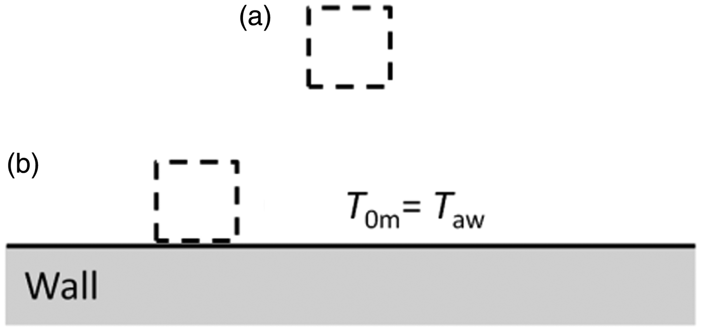

Adjacent to the wall (b), in case of an adiabatic wall and incompressible conditions, the adiabatic wall temperature, $T_{aw}$ , is equal to the mixed-out total temperature within the cell, $T_{0 m}$ . We write $T_{aw} = T_{0 m}$ . With this substitution in equation (7), we observe that this is the equation for film effectiveness. That is

\sum_{i} φ_{i} = \frac{T_{0 \infty} - T_{aw}}{T_{0 \infty} - T_{0 c}} = η

(8)

i.e. the film effectiveness in a particular cell is equal to the coolant mass fraction (

η = \sum_{i} φ_{i}

). The argument is valid only if the scalar field (the scalar concentrations) mimics the thermal field, which develops on account of both advection and diffusion, including turbulent terms.

The steady-state advection–diffusion energy equation is

\nabla \cdot (ρ \vec{u} c_{p} T) = \nabla \cdot (k_{eff} \nabla (c_{p} T))

(9)

where

\vec{u}

is the velocity vector, where ρ,

c_{p}

, and T have their normal meanings, and where

k_{eff}

is the effective turbulent thermal diffusivity, defined by

k_{eff} = k + (\frac{c_{p} μ_{T}}{P r_{T}})

(10)

where k is the thermal conductivity,

μ_{T}

is the turbulent viscosity, and

P r_{T}

is the turbulent Prandtl number.

In the scalar tracking method, to ensure that the scalar field mimics the thermal field, a transport equation is defined for each scalar, $φ_{i}$ , that has the same form as the advection–diffusion energy equation. We write

\nabla \cdot (ρ \vec{u} φ_{i}) = \nabla \cdot (Γ \nabla φ_{i})

(11)

where Γ is the scalar diffusivity, which (to mimic the thermal field) is set equal to the effective turbulent thermal diffusivity,

Γ = k_{eff}

. In this case, the ratio between the turbulent thermal diffusivity and the scalar (mass) diffusivity (i.e. the Lewis number,

Le

) is set equal to 1.

Equation (8) allows the overall cooling effectiveness to be calculated from the sum of the scalar variables. This, on its own, is not beneficial. The advantage of the method, however, is that by examining the scalar concentrations in the downstream flow the individual contribution from each hole can be calculated at every point in the downstream flow field. By extracting these concentration fields, individually for each cooling hole, a proxy model can be built allowing rapid optimization out of the CFD loop, with occasional recalibration against CFD. The proxy model can have any desired level of complexity, ranging from linear (with mass flow rate) to more sophisticated models which include some level of flow modelling.

In this paper, we demonstrate the method using ANSYS-CFX for CFD solutions. Additional scalar transport equations were defined by using a script written in CEL – a Perl-based CFX programming language. The scalar concentration fields were extracted from each converged CFD solution and fed into a proxy model written in Matlab. Optimization steps were conducted in the proxy model, before being handed back to CFD for recalibration. The process is now described in detail.

Combined scalar tracking CFD and MOGA method

In this section, we present the combined scalar tracking, CFD, and MOGA method.

At high level, the principle of the method is to use a proxy model (implemented in Matlab) of the film cooling system in a MOGA optimization routine and periodically calibrate the proxy model against a high-fidelity CFD solution. We refer to MOGA/proxy model combination as the inner loop and to the high-fidelity CFD as the outer loop. The two loops are converged together, but with many thousands of iterations in the inner loop and a small number of iterations in the outer loop. Periodic recalibration keeps the inner loop from diverging from the outer loop, and therefore means the proxy model remains a reasonable representation of the flow system throughout the convergence process. Because the inner and outer loops are converged together, the residual between the two is small in the final step, and the final design is confirmed with CFD. The process is similar to conventional MOGA-CFD optimization processes, but with savings of many orders of magnitude in computational cost. We now describe the model in detail.

Defining the objective functions

Objective functions are defined, which set the target to optimize against. In our example, below, we seek to maximize component life and minimize aerodynamic loss, so generate two objective functions addressing each of these targets. As with all automated optimization routines, the definition of this function determines the outcome of the optimization.

Defining and initializing the proxy model with a first CFD solution

The scalar tracking method is implemented in CFD to identify the contribution to the overall film effectiveness distribution of the flow from a particular film cooling hole. In the proposed method, an initial CFD simulation is run on a first generation design to evaluate both the individual scalar concentrations (in the entire downstream field, if desired) and the individual hole mass flow rates. These are then used to initialize the proxy model which at the first iteration gives (by definition) identical results to the CFD simulation, and in subsequent iterations allows extrapolation via linear superposition to provide a rapid means of design optimization. The proxy model can be line-based (targeting an individual axial plane downstream) or full-surface, depending on the fidelity of the prediction required.

Defining the exchange rate between hole diameter and mass flow rate

For the case of a film cooling optimization for a system with fixed internal pressure (analysis of a coupled system would follow by extension of the method), the hole diameter and position are variables to be adjusted (iterated) by the MOGA to optimize against the target function. This requires a model that estimates the change in contribution to the film effectiveness when the hole diameter and/or position are changed. In the present study, we used a compressible flow model of a hole, with discharge coefficients determined on a per-hole basis from CFD. The discharge coefficient was recalibrated at every outer-loop iteration of the process. In principle, any reasonable model can be used. The coolant feed total pressure was the same for all holes and the external static pressure was determined from the CFD solution and the proxy model recalibrated at every CFD (outer loop) step.

Defining the effectiveness contribution for new hole locations

In systems where hole location is included as a variable, the effectiveness field associated with a new (or moved) hole location could be determined as a linear interpolation of the effectiveness contributions from nearest neighbour holes, weighted appropriately for mass flow rates. In the current study, this step was omitted but is a natural extension of the method.

MOGA extrapolation of the proxy model

Once the proxy model is generated and initialized, and the exchange rates for hole diameter and mass flow are defined, a MOGA optimization is performed on the proxy model. In this scheme the hole mass flow rates (varied using the diameter) are adjusted using the MOGA algorithm to improve the fitness of the solutions as measured by the objective function. The MOGA optimization is performing an extrapolation, and this is only as good as the proxy model. In our example, we have a simple superposition model, which is accurate for small extrapolations, but increasingly inaccurate where flow rates are changed by an amount that might affect the overall flow structure (there is no physical model of this in the proxy model). To stabilize the solution, we restrict the extrapolation that is allowed within a single convergence period of the proxy model. For multi-objective problems, the MOGA process generates a Pareto front of so-called Pareto-optimal designs. One design must be – somewhat arbitrarily – chosen from this front and will be passed to the outer loop for recalibration with a CFD model. Different strategies can be taken, and we discuss a particular example later in this paper.

CFD validation of the MOGA/proxy model output

After convergence of the inner loop (MOGA algorithm and proxy model), the chosen (‘fittest’) design is passed to the outer loop and a CFD simulation performed. The results of the CFD simulation, measured in terms of the objective functions, are compared to the optimizer prediction. Provided the proxy model is sufficiently accurate over the extrapolation distance, the fitness of the CFD solution will be improved over the previous design.

Stability check of the proxy model over a particular outer-loop iteration

The accuracy of the proxy model over the extrapolation distance can be assessed by comparing the differences in film effectiveness between the previous-generation and current-generation designs as predicted by the proxy model and the CFD model. If the differences are similar, the proxy model was stable over the extrapolation distance. An example of this check is given later in the paper.

Recalibration of the proxy model

The following information is now extracted from the CFD solution, for the purpose of recalibrating the proxy model: the external static pressure distribution, individual hole mass flow rates, passive scalar concentration field. Once the proxy model is recalibrated, it will be an exact representation of the current-generation CFD solution. The MOGA/proxy model routine (inner loop) is now iterated to convergence to define the next generation design. The process is then repeated until the converged solutions cannot be improved as measured by the objective functions. The process is shown schematically in the flow chart of Figure 2.

Figure 2.

Flow chart of the combined scalar tracking, CFD, and MOGA method. The dashed line represents the next step (in relation to the numbering in the blocks, i.e. the pause point) of the process. CFD: computational fluid dynamics; MOGA: multi-objective genetic algorithm.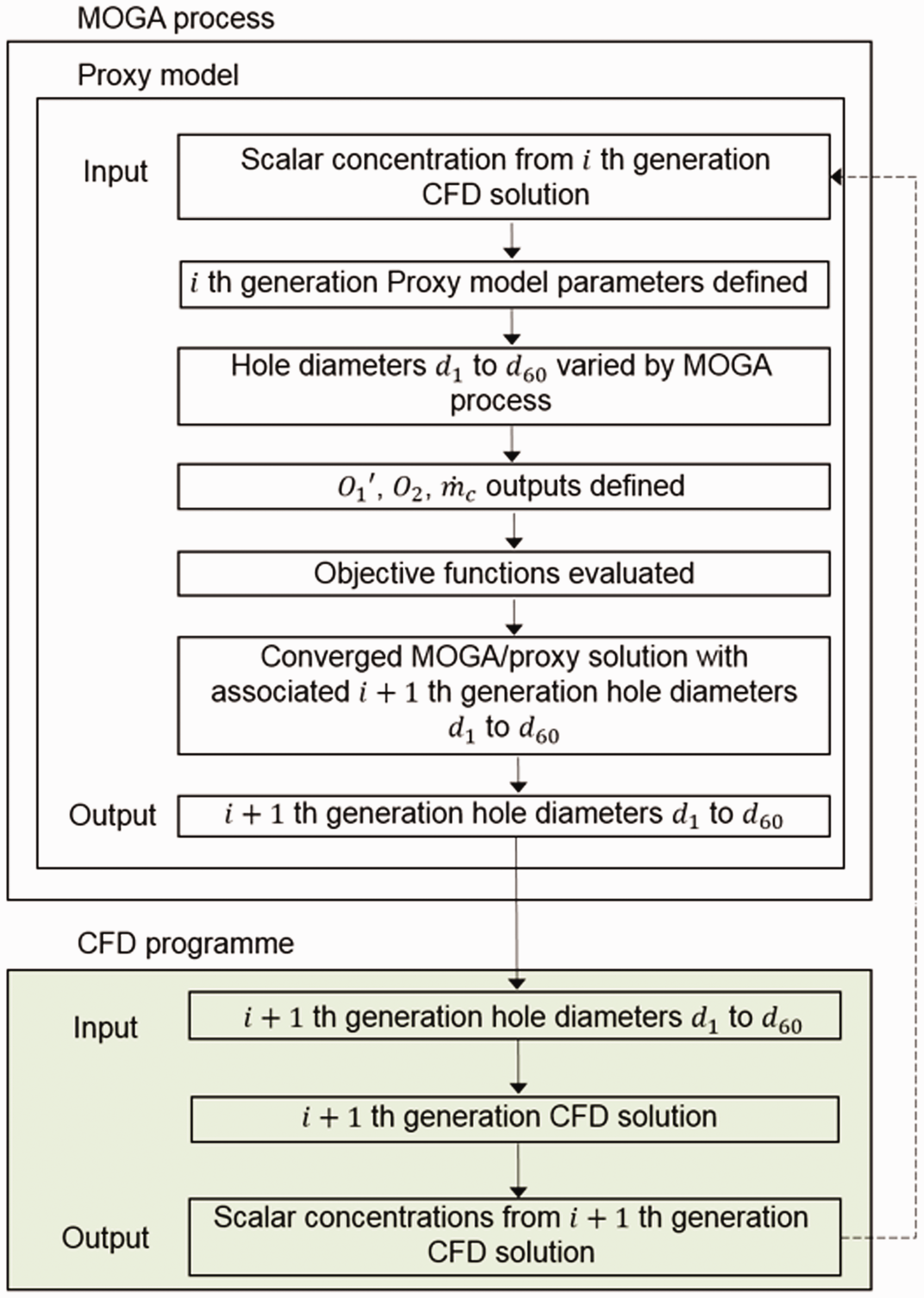

Flat plate test case

In this section, we describe the test case used to demonstrate the proposed optimization method. We first describe the general design of the test case and then discuss the application of the proposed method to the particular example.

General design of the flat plate test case

The isentropic relations were used to perform a preliminary assessment of the flow variables changes along the length of the test case domain (see Figure 5). The domain has a length given by $l / d$ = 125, contracting linearly from a passage height of $h_{i} / d$ = 25 to $h_{o} / d$ = 12.5. This gives rise to flow acceleration along the axial length of the domain. Mixing losses depend on the local Mach numbers (both coolant and mainstream). The inlet and exit Mach numbers were approximately 0.2 and 0.5, respectively. Figure 3 shows the predicted streamwise distributions of pressure ratio, $p / p_{0 \infty}$ ; Mach number, M; temperature ratio, $T / T_{0 \infty}$ ; and ratio of local area to inlet area, $A / A_{max}$ . The resulting momentum flux ratio, I, for a coolant-to-mainstream pressure ratio $p_{0 c} / p_{0 \infty}$ = 1.01 is also shown. This varies in the range 1.06 $< I <$ 1.30. The same uniform value of total pressure was imposed at all cooling hole inlet planes (condition similar to the constraint in an engine). The total pressure was kept constant throughout the optimization process. Thus, notwithstanding local effects caused by cross-flow, the coolant-to-mainstream momentum flux ratio was held constant during the optimization process. Individual hole mass flow rates were varied by adjusting the hole diameters.

Figure 3.

Axial distribution (from domain inlet to outlet) of flow variables predicted by isentropic equations for the test case shown in Figure 5.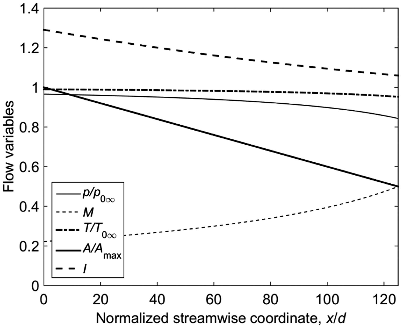

The Sellers model¹³ was employed for rapid preliminary assessment of the adiabatic film effectiveness distribution resulting from a multi-row film cooling configuration. The objective was a flat plate cooling design with a minimum distance between two rows of holes that would allow for substantial mixing of the films (see later discussion) between each row. As we discuss later (see discussion regarding limitations of the proposed optimization technique), this reduces the chance of discrepancies between the proxy model and CFD recalibration step resulting from local changes in flow field caused by strong interaction of holes. It is not a requirement for the method that such interactions are limited, but it makes the convergence process easier to interpret (extended discussion in later section).

To initialize the Sellers model, a 3D CFD simulation was run for a single hole. The coolant plenum was fully resolved in the CFD model. The hole was (somewhat arbitrarily, as the flow is accelerating) set to have a momentum flux ratio of I = 1.06, equivalent to an axial coordinate of $x / d$ = 125 in Figure 3. The hole inclination angle was 30° to the surface. The domain width was set to $y / d$ = 10, with periodic walls. In the CFD the domain length was set to 50 d to allow for substantial mixing of the film. The domain had 2.60×10⁶ cells and was run with a second order, steady state, compressible solver. The $k - ω$ SST was selected for turbulence closure. Results from the CFD prediction are shown in Figure 4 (dashed red line) as a distribution along the hole centreline. An extrapolation of the CFD distribution (based on exponential decay) was performed to extend the results to 125 d. The extrapolation is shown as a solid red line. The Sellers model was used to predict the film effectiveness distribution arising from a number of rows of holes.

Figure 4.

Streamwise distribution of film effectiveness along the hole centreline for: a single hole CFD prediction (dashed red line), an extrapolated single hole CFD prediction (solid red line), and a prediction of the superposition of three rows using the Sellers method (for a row spacing of 25 d). CFD: computational fluid dynamics.

Figure 5.

Diagram of the computational domain: (a) side view and (b) plan view, showing initial film effectiveness distribution.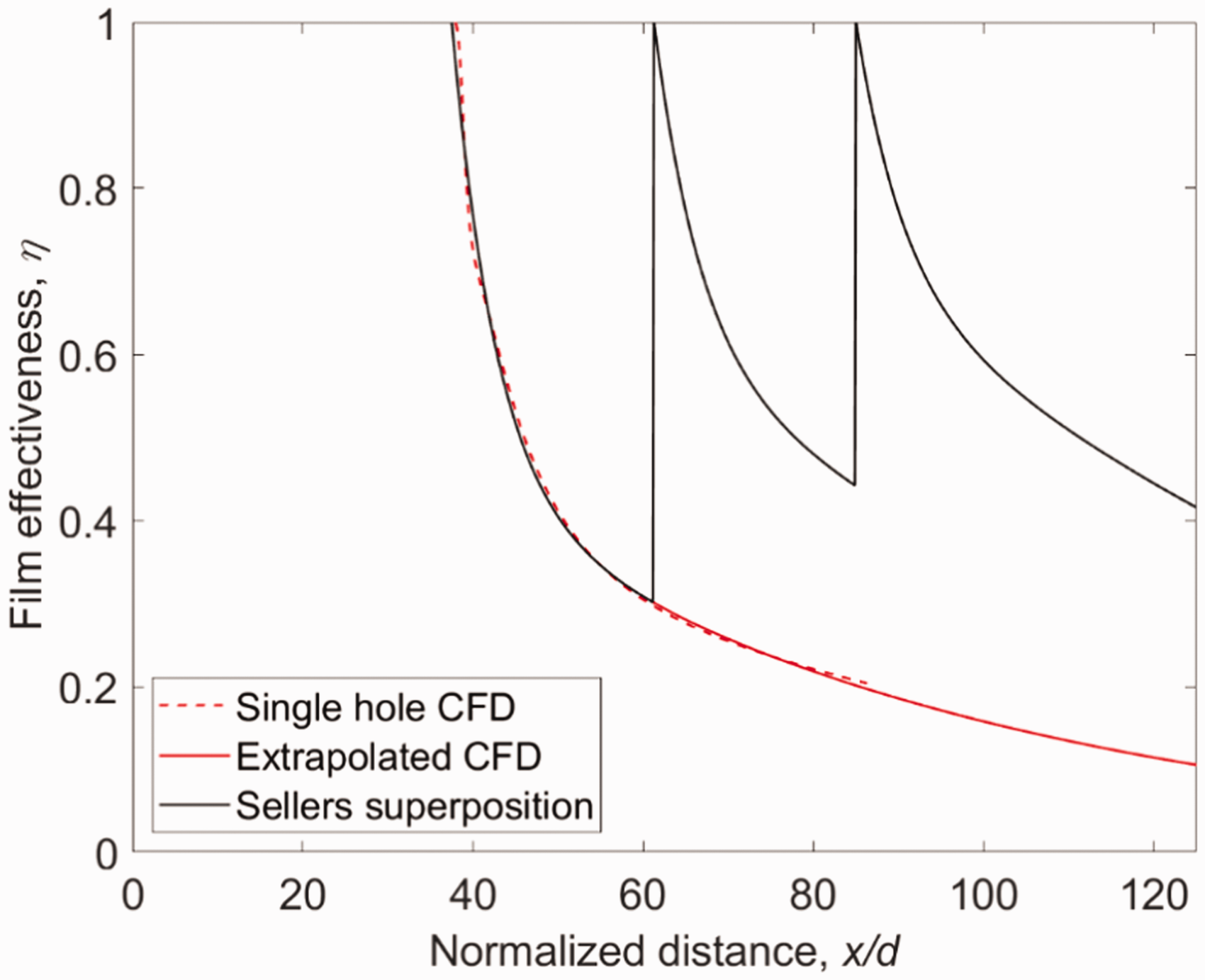

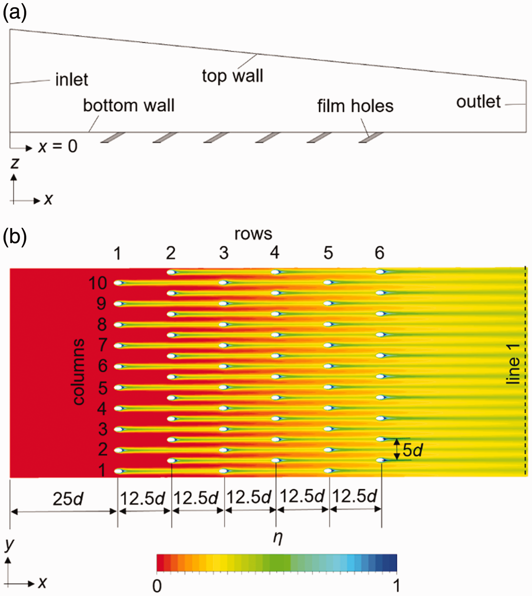
Based on the superposition results of Figure 4, a uniform streamwise spacing between aligned rows of approximately $x / d$ = 25 was chosen to allow for substantial mixing-out of coolant between rows, ensuring minimal hole-to-hole interactions (see later section).

The hole spacing in the lateral direction, y, was chosen so as to ensure minimal hole-to-hole interaction effects up to a streamwise distance of 50d. By visually inspecting the CFD results used to seed the Sellers model (domain width of $y / d$ = 10) a lateral spacing of $y / d$ = 5 was observed to be sufficient to meet this requirement.

A development length at the domain inlet was somewhat arbitrarily set to $x / d$ = 25 to allow for a boundary layer to establish. Likewise, at the domain exit a distance of $x / d$ = 37.5 was allowed for the last row to partially mix out.

The final configuration is shown in Figure 5. A staggered row configuration with $y / d$ = 5, and $x / d$ = 25 between aligned rows – or $x / d$ = 12.5 between staggered rows – was chosen. To identify particular holes in later sections, we refer to the row and column number of individual holes. There are 60 holes in total, organized into six rows of 10 holes each.

The flow properties and geometrical details of the computational domain are summarized in Table 1.

Table 1.

Flow properties and geometrical parameters of the computational domain.

Parameter	Value
Inlet Mach number	0.20
Outlet Mach number	0.50
Reynolds number based on d	12,981
Domain inlet height, $h_{i} / d$	25
Domain outlet height, $h_{o} / d$	12.5
Domain width, $w / d$	50
Domain length, $l / d$	125

Defining the objective functions

In this study, we are interested in both component life and aerodynamic loss. We thus have two objective functions which we now consider in turn.

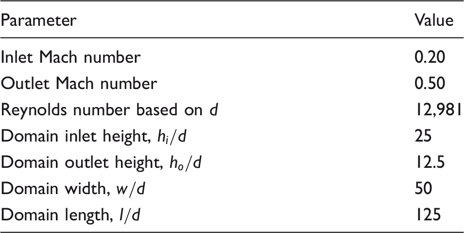
Component life is related to surface temperature. We consider the difference between the local wall temperature $T (x, y)$ and a target temperature $T_{t} (x, y)$ . Somewhat arbitrarily we define the life objective function as follows

\begin{matrix} O_{1} = 1 - 1 / L for T (x, y) - T_{t} (x, y) > 0, \\ O_{1} = 0 for T (x, y) - T_{t} (x, y) < 0 \end{matrix}

(12)

where L is a non-dimensional oxidation life, defined so that for every 20 K over the target temperature, the expected life halves. That is

L = \frac{1}{2^{(T - T_{t}) / 20}}

(13)

This relationship for oxidation life is representative of the typical engine situation for hot components. The characteristic of the objective function is such that undercooling ( $T > T_{t}$ ) is heavily penalized, but overcooling ( $T < T_{t}$ ) is not favoured. The expression (12) is plotted in Figure 6.

Figure 6.

Life objective function, 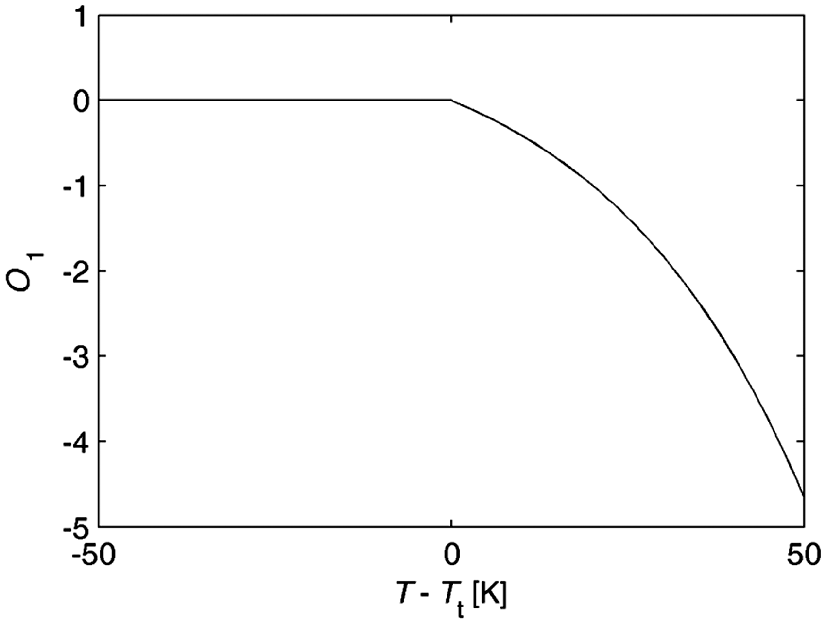$O_{1}$ , as function of $T - T_{t}$ .

We note that for our adiabatic case, the difference between surface temperature and target temperature can be expressed in terms of the adiabatic film effectiveness, thus

T (x, y) - T_{t} (x, y) = (η_{t} (x, y) - η (x, y)) (T_{0 c} - T_{0 \infty})

(14)

where

η_{t} (x, y)

is defined by

T_{t} (x, y)

– or vice versa – and

η (x, y)

can be calculated from equation (8).

In general, such an optimization would consider the entire surface and form part of a coupled solution in which the contribution of an internal cooling system was also accounted for. In our simple example, we set a target film effectiveness distribution at only a single axial location (approximately $x / d$ = 35 downstream the last row of holes) as follows

\begin{matrix} η_{t} = 0.40 for 0.0 \leq y^{*} < 0.5 and x / d = 35, \\ η_{t} = 0.20 for 0.5 \leq y^{*} \leq 1.0 and x / d = 35 \end{matrix}

(15)

where

y^{*}

is the normalized lateral coordinate. Although simple, this distribution is an interesting test exercise for the optimization process, because the initial solution is chosen to have both overcooled and undercooled regions. To reduce the objective function to a single value for each solution, for a given iteration of the solution, we take the minimum value of

O_{1}

. We refer to this as

O_{1}'

We now consider the film cooling loss objective function. We include two elements: the kinetic energy loss due to aerodynamic mixing and the thermodynamic loss due to heat transfer between coolant and mainstream.

We conceptualize a mixing layer in which a coolant flow rate, ${\overset{\cdot}{m}}_{c}$ , is mixing with a mass flow rate of entrained mainstream gas, ${\overset{\cdot}{m}}_{e}$ . This is shown in Figure 7. To perform a mixing calculation, we need to define ${\overset{\cdot}{m}}_{e}$ . In a particular calculation, we do this by defining ${\overset{\cdot}{m}}_{e}$ such that were the hypothetical mixing layer fully mixed, the adiabatic film effectiveness η would take a value equal to the maximum value seen at the interrogation line for that particular solution. In fact, for $η < 0.4$ (which is true for most of our solutions), the loss is relatively insensitive to the particular value of η we take to define ${\overset{\cdot}{m}}_{e}$ .

Figure 7.

Schematic of the mixing layer.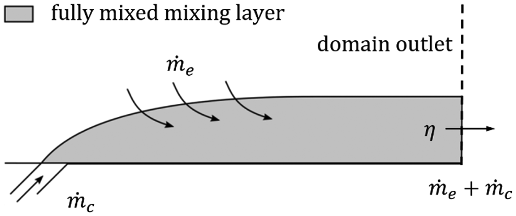

Once ${\overset{\cdot}{m}}_{e}$ is defined for a particular solution, we compute the Mach number and total pressure of the mixed-out layer using the control volume method of Hartsel.⁷ In our application of the model, friction is neglected and both fluids are modelled as perfect gases with the same specific heats, independent of temperature. We also assume that the mainstream velocity at the injection location (on which the total pressure loss depends) is unaffected by coolant injection. In more complex models (e.g. Kollen and Koschel⁸) it is possible to account not only for the local Mach number (the primary factor affecting loss) but also for the acceleration of the mixing layer to a given (generally higher) outlet Mach number (e.g. the Mach number at the exit of a turbine cascade). In our situation, the outlet Mach number is unchanged through the optimization, so more sophisticated models were seen as an unnecessary complication.

The Hartsel model⁷ solves for continuity, momentum, and energy in an assumed constant pressure ( $p_{m} = p_{\infty}$ ) mixing process. The resulting expression for the mixed-out layer Mach number, $M_{m}$ , is

M_{m}^{2} = (\frac{(1 + Y_{c}) (T_{0 \infty} + Y_{c} T_{0 \infty}) (1 + \frac{γ - 1}{2} M_{\infty}^{2})}{(Y_{c} \frac{u_{c}}{u_{\infty}} cos α + 1) M_{\infty}^{2} T_{0 \infty}} - \frac{γ - 1}{2})^{- 1}

(16)

where

M_{\infty}

is the freestream Mach number at the injection point,

u_{c}

and

u_{\infty}

are the coolant and freestream velocities at the injection point, respectively,

Y_{c} = (ρ_{c} u_{c} A_{c}) / (ρ_{\infty} u_{\infty} A_{\infty})

, and α is the hole inclination angle with respect to the x direction.

Assuming that $p_{m} = p_{\infty}$ , the ratio of the total pressure in the mixed-out state to the freestream total pressure can be shown (see Kollen and Koschel⁸) to be given by

\frac{p_{0 m}}{p_{0 \infty}} = \frac{(1 + \frac{γ - 1}{2} M_{m}^{2}) \frac{γ - 1}{γ}}{(1 + \frac{γ - 1}{2} M_{\infty}^{2}) \frac{γ - 1}{γ}}

(17)

The overall entropy production rate due to irreversibility associated with total pressure loss introduced by film injection is calculated as follows

Δ {\overset{\cdot}{S}}_{KE} = - ({\overset{\cdot}{m}}_{c} + {\overset{\cdot}{m}}_{e}) R \sum_{i} ln (\frac{p_{0 m}}{\frac{{\overset{\cdot}{m}}_{e} p_{0 \infty} + {\overset{\cdot}{m}}_{c} p_{0 c}}{{\overset{\cdot}{m}}_{e} + {\overset{\cdot}{m}}_{c}}})_{i}

(18)

where

{\overset{\cdot}{m}}_{c}

is the coolant mass flow rate and

{\overset{\cdot}{m}}_{e}

is the mass flow rate of (‘entrained’) mainstream fluid that has entered the control volume. The term in parentheses is the ratio of the total pressure in the mixed-out layer to the mass flow averaged mean inlet total pressure for flow entering the control volume of the mixing layer.

In our loss model, we also include the contribution due to thermal mixing loss, or entropy production rate due to heat transfer between coolant and mainstream. This term was derived by Young and Wilcock⁹ and is given by the following equation

Δ {\overset{\cdot}{S}}_{Q} = {\overset{\cdot}{m}}_{c} \int_{T_{c}}^{T_{m}} c_{p} (\frac{1}{T} - \frac{1}{T_{m}}) d T

(19)

where

{\overset{\cdot}{m}}_{c}

is the coolant mass flow rate, and

T_{c}

and

T_{m}

are the coolant and mixed-out temperatures, respectively.

c_{p}

is the specific heat capacity at constant pressure and takes the same value for coolant and mainstream flows in our simulations. We integrate equation (19) for a perfect gas. This yields the following

Δ {\overset{\cdot}{S}}_{Q} = {\overset{\cdot}{m}}_{c} c_{p} (ln \frac{T_{m}}{T_{c}} + \frac{T_{c}}{T_{m}} - 1)

(20)

Our film cooling loss objective function combines the two sources of loss

O_{2} = Δ {\overset{\cdot}{S}}_{KE} + Δ {\overset{\cdot}{S}}_{Q}

(21)

In picking solutions from the Pareto front, we seek to maximize the life function,

O_{1}

, and minimize the film cooling loss objective function,

O_{2}

CFD setup and initialization of the proxy model

CFD simulations were performed with ANSYS-CFX. Mainstream gas and coolant were simulated as ideal gases with gas properties. The $k - ω$ SST turbulence model was selected for the turbulence closure, with second order space discretization. Steady-state simulations were performed. Using the method described above, the coolant concentration of each cooling hole was computed by associating a unique scalar variable with the flow from each hole and solving an additional passive-scalar transport equation. The scalar transport equations were defined by using the pre-processing software CFX-Pre. The values of the passive scalars, $φ_{i}$ , were set to unity at the inlets of the corresponding cooling holes (denoted i) and to zero at all other inlets. Domain inlet total pressure and temperature conditions were specified, as well as the value of the turbulent intensity. A static pressure value was imposed at the domain outlet, and symmetry boundary conditions were set on both sides of the computational domain.

The computational grid was generated by using BOXERMesh and had 16.9 × 10⁶ tetrahedral and hexahedral elements. A detailed view of the surface mesh is shown in Figure 8(a), and a detail of a lateral cut through a cooling hole in Figure 8(b). The grid resolution on the cooled wall and film holes was increased to resolve high temperature gradients. The near wall region was refined with 12 prism layers with an expansion ratio of 1.2. The value of the area-averaged normalized wall distance (based on Re) was below 5 over all wetted surfaces (Figure 9(a)).

Figure 8.

(a) Plan view of the cooled-wall surface mesh and (b) lateral view of the mesh.

Figure 9.

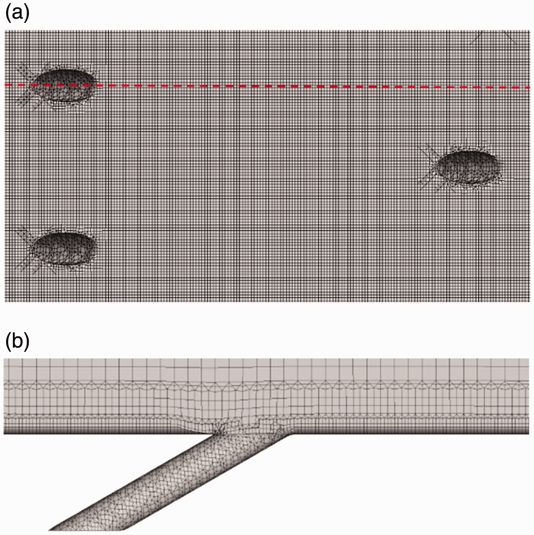
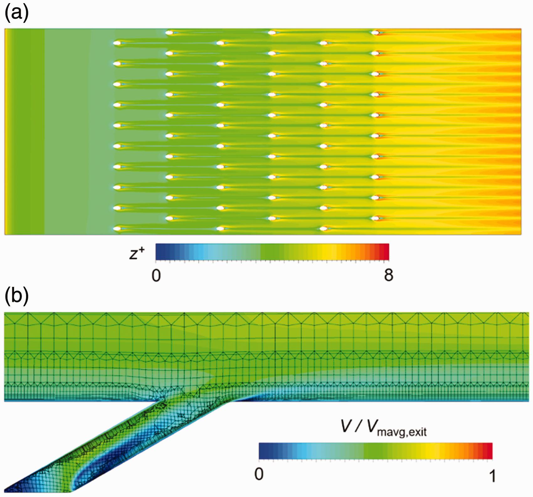
(a) Contours of $z^{+}$ on the wall surface and (b) contours of normalized velocity magnitude ( $V / V_{mavg, exit}$ ) on a plane through a centre-hole.

Figure 9(b) shows contours of velocity normalized by the mass-averaged value at the domain exit on a plane through a centre-hole ( $V / V_{mavg, exit}$ ). The local mesh is shown to be sufficiently refined to capture the velocity gradients in the near wall region.

Defining the exchange rate between hole diameter and mass flow rate

The exchange rate between hole diameter and mass flow rate was estimated by the following equation for compressible flows

{\overset{\cdot}{m}}_{i} = C_{d} \frac{π d_{i}^{2} p_{0}}{4 \sqrt{T_{0}}} \sqrt{\frac{γ}{R}} M (1 + \frac{γ + 1}{2} M^{2})^{- \frac{γ + 1}{2 (γ - 1)}}

(22)

where

p_{0}

is the stagnation pressure,

T_{0}

is the stagnation temperature, M is the Mach number, γ is the isentropic exponent, R is the specific gas constant, and

C_{d}

is the discharge coefficient. The discharge coefficient is calculated by using the previous CFD solution of each global iteration (or outer loop). The discharge coefficient is assumed to be constant within a given MOGA run (or inner loop). We later demonstrate that this approximation is accurate for the range of extrapolation allowed within each MOGA run (see Figure 11 and associated discussion).

Details of the MOGA algorithm used in the present example

The JEGA evolutionary algorithm library, developed within the DAKOTA (C++ based, open source platform¹⁰) software, was used. GAs are widely exploited for function optimization. The GAs are so-called because they mimic the evolution process of biological systems in nature. During the optimization, populations of ‘genomes’ are generated and individuals with the highest fitness are selected for the next population. In GAs, each individual is a binary string which represents a design. Natural processes such as crossover and mutation are simulated in GAs via recombination of bits within binary strings. In particular, crossover is performed through the construction of a new child genome using portions of two or more parent genomes. Without mutation, genomes may become too similar and the process may be slowed or even trapped in local minima.

For the present work, the MOGA algorithm developed by Eddy and Lewis¹¹ was employed. This is a rank-based fitness assignment algorithm for multi-objective optimization problems.¹² Unlike single objective strategies, the optimal solutions of a multi-objective optimization are a Pareto front formed by designs for which none of the objective functions can be improved without degrading one of the other objectives. Designs belonging to the Pareto set are called non-dominated or Pareto optimal.

Figure 10 shows the MOGA flow chart for our optimization process. The proxy model is initialized with data from the first CFD run, with the passive scalar values associated with each cooling hole. In our simple example, we consider the value of these scalars at a single downstream line ( $x / d$ = 35 from the last cooling row). The flow conditions ( $M (x, y)$ , $p_{0 \infty}$ , $p_{0 c}$ , $T_{0 \infty}$ , $T_{0 c}$ , $p (x, y)$ ) are specified using the first CFD solution (for the purpose of loss calculation). The MOGA optimizer starts by performing random sampling to obtain the initial set of mass flow rates to generate a first population. The minimum of the life objective function, $O_{1}'$ , and the coolant loss objective function, $O_{2}$ , are then computed at the interrogation line. This process is repeated until a pre-defined population size is reached. The fitness of each design is calculated based on its values of $O_{1}'$ and $O_{2}$ . Only the designs with the highest fitness are selected and passed to the next population. The process is repeated until the convergence criteria of the MOGA are met – typically that the change in the Pareto front between iterations falls below a user specified threshold. In our particular case, the threshold was set to 0.1%.

Figure 10.

Block diagram of the MOGA process (breakdown of the blocks included in the inner loop of Figure 2).

Figure 11.

Evolution of the Pareto front between successive generations of the MOGA algorithm. Results are normalized by the initial MOGA population.

Figure 12.

The residual in between the beginning and end of each global iteration, shown as: maximum-to-minimum variation across all holes (red shaded area); and RMS of the residual. RMS: root mean square.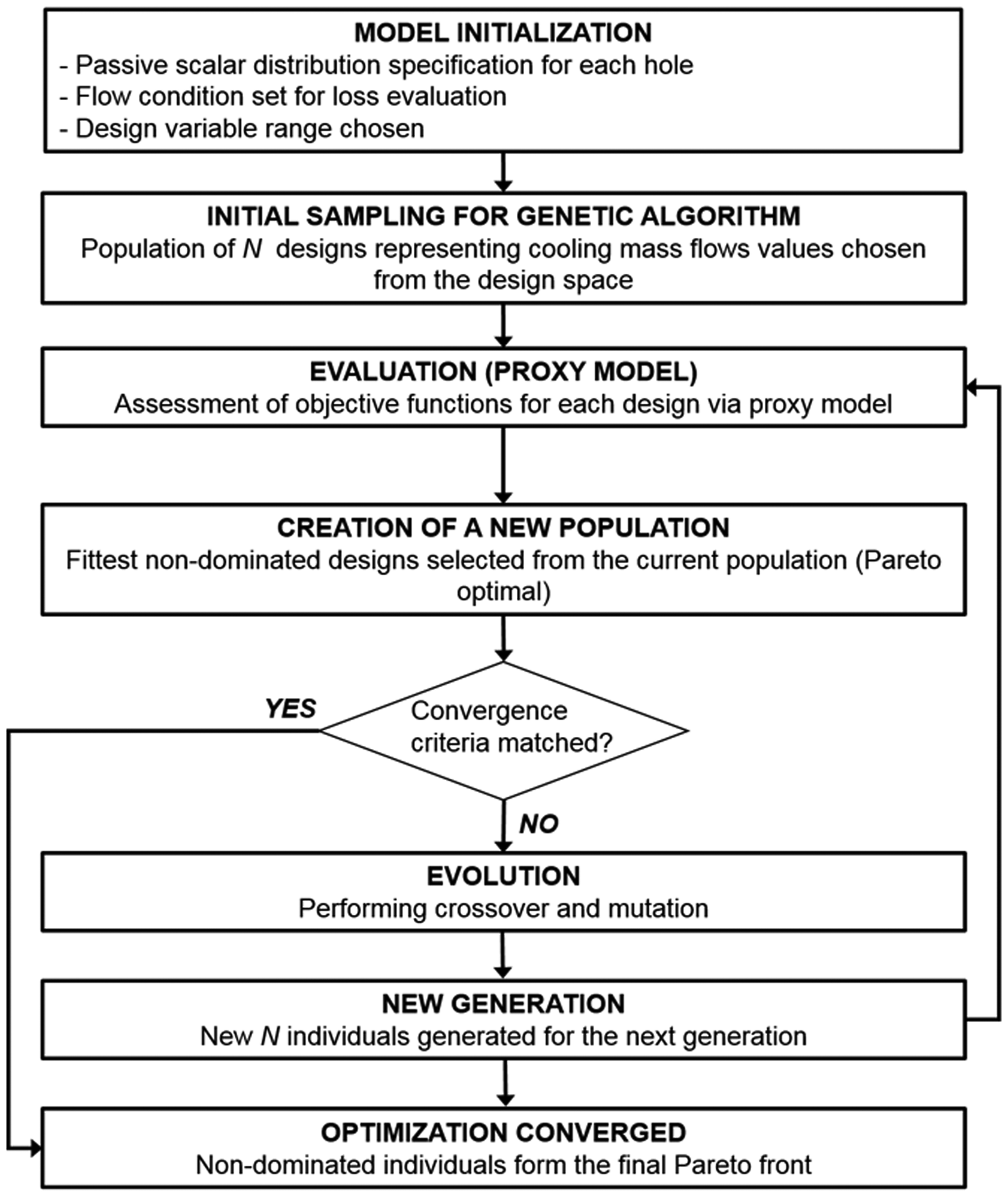

The MOGA decision-making optimization core used the DAKOTA software, which runs in C++, and was linked to the Matlab-implemented proxy model via UNIX shell scripting. We now describe the DAKOTA MOGA in more detail.

The MOGA optimization was controlled with the DAKOTA input file (dakota.in), which contains parameters defining environment, method, model, variables, interface, and responses. These sections of the program are fully defined in Adams et al.¹⁰ The method parameters dictate population size, crossover technique, mutation technique, mutation rate, and convergence criteria. Convergence of the algorithm was typically reached within 3 h for each MOGA run (10 simultaneous evaluations on a 3.40 GHz Linux station). The maximum population size was set to 500 designs. Crossover was performed with shuffle random technique with two parents and crossover rate of 0.8. Mutation occurred by means of the replace uniform technique with a mutation rate of 0.1. The variables were set to be continuous (mass flow rate allowed to vary continuously) but with upper and lower bounds set to 0.8 and 1.2 of the initial value, respectively. These limits are to prevent excessive extrapolations of the MOGA routine, which go too far outside the approximately linear range based on the previous CFD recalibration step. The responses parameters define the objective functions.

Results and discussion

In this section we consider the results of the optimization of the cooling system depicted in Figure 5 with the dual targets of maximizing component life and minimizing loss associated with coolant introduction.

General results

We recall that the life target is based on the somewhat arbitrary adiabatic effectiveness distribution shown in Figure 15, which was chosen so that in the first design, parts of the plate are both undercooled and overcooled. The target effectiveness distribution is hard to interpret in terms of life in isolation, as it would normally form part of a system with an internal cooling arrangement. The objective functions effectively minimize the difference in adiabatic film effectiveness from a target distribution defined at the domain exit line whilst minimizing the total entropy generation (both aerodynamic and thermodynamic) associated with film cooling mixing. The target distribution at the domain exit ( $x / d =$ 35 from the last row of holes) is given in equation (12) (see also Figure 15).

Figure 11 shows an example of the evolution of the Pareto front for a MOGA run, showing snapshots from every 20th population, up to population 120. It can be seen that around population 120, the MOGA process is converged (for this particular case), and there is little development of the Pareto front. As with all multi-objective optimization processes, there is no single ‘best design’ on the Pareto front, and a somewhat arbitrary choice must ultimately be. In the figure we present the data for a typical MOGA run, normalized by the initial values ( $O_{1, ini}'$ and $O_{2, ini}$ ).

The Pareto front converges towards decreasing values of both $O_{1}' / O_{1, ini}'$ (x-axis) and $O_{2} / O_{2, ini}$ (y-axis). An increase in the value of $O_{1}'$ (i.e. $O_{1}'$ becomes less negative over time, leading to a lower ratio $O_{1}' / O_{1, ini}'$ ) represents increasing life. Likewise, a decrease in the value of $O_{2}$ (a positive quantity) represents decreasing loss.

In this optimization, we manually selected designs from approximately the centre of the Pareto front. This selection strategy was applied consistently for each MOGA run.

At each stage, the chosen design was passed to the next global iteration: first being passed to the CFD, with the information being passed back to the proxy model by way of recalibration.

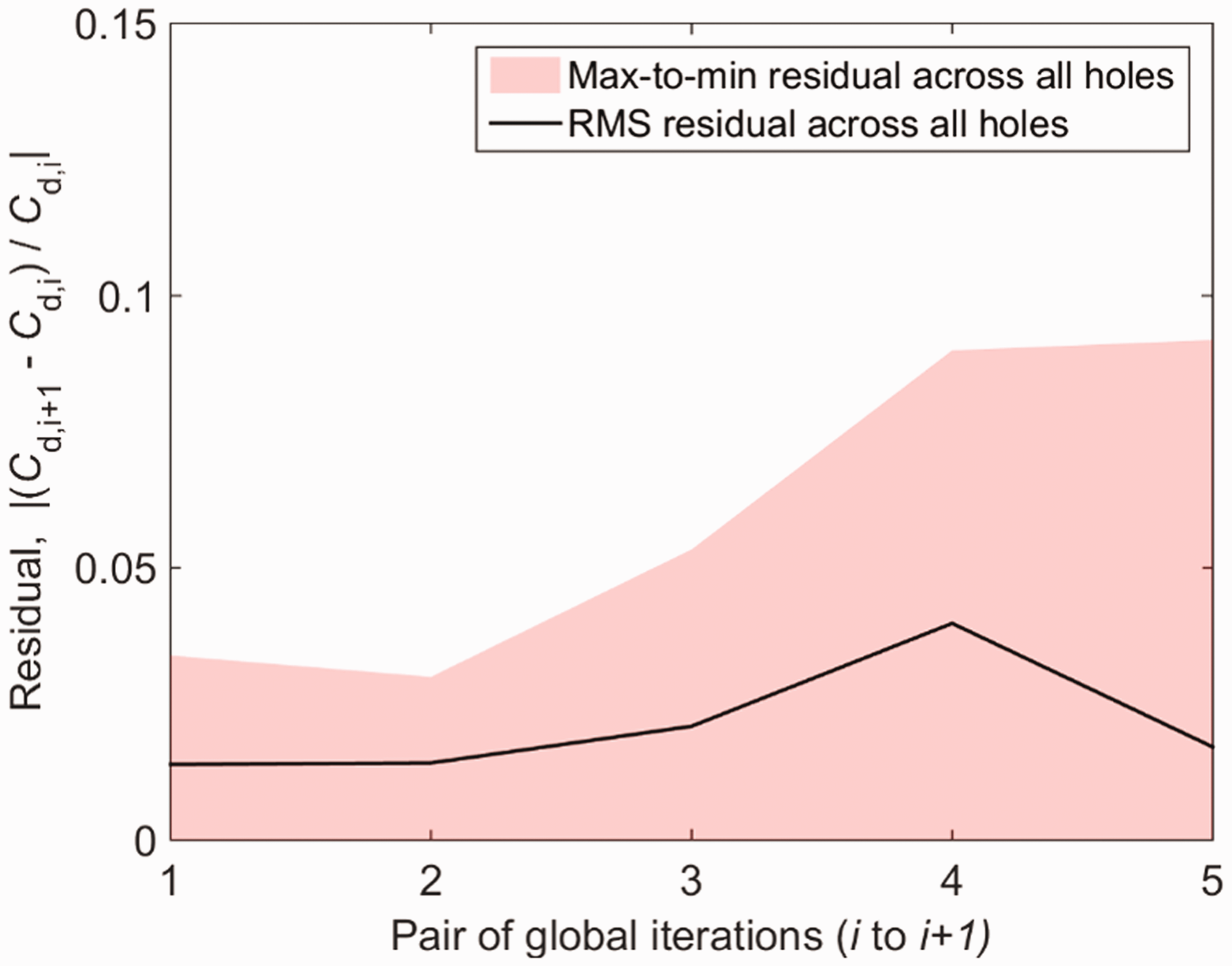
During each MOGA loop, the coolant mass flow rates are continuously adjusted using the method described in relation to equation (20). In this equation, the discharge coefficient, $C_{d}$ , is defined from the CFD solution from the previous calibration step and kept constant within a given MOGA run. That is, in a given MOGA run, there is a linear relationship between mass flow rate (adjusted by the MOGA) and hole area (an output from the MOGA passed to the next CFD calibration step). At the end of the MOGA run, the updated hole areas (and associated diameters) from the chosen solution are passed to the next CFD recalibration step. The new CFD-predicted mass flow rates are then compared to the mass flow rates from the selected MOGA solution.

To assess the divergence in mass flow rate (difference between CFD and proxy model) introduced between the beginning and end of an individual global iteration, as a result of assuming constant $C_{d}$ within that global iteration (we note that the solution is recalibrated at the start of the next global iteration), we consider – for each hole – the ratio of the $C_{d}$ between each pair of global iterations (1–2, 2–3, and so forth). This ratio represents the divergence that has occurred by the end of the proxy model optimization as a result of incorrectly assuming constant $C_{d}$ . Figure 12 shows that for each pair of global iterations, the RMS, maximum and minimum values of the ratios of $C_{d}$ between the ith and i + 1th global iterations are presented as the residual $(C_{d, i + 1} - C_{d, i}) / C_{d, i}$ . The RMS of the residual is below 4% for every pair of global iterations, suggesting reasonable accuracy of the assumption of constant $C_{d}$ within a global iteration. For completeness, we note that the change in individual hole area was constrained to a proportional increase of 20% for an individual global iteration.

We now consider the results of the MOGA optimization process, first considering the film effectiveness (life objective function) and then the entropy rise associated with mixing.

The overall film effectiveness distribution at the end of the optimization process (after six global runs) is shown in Figure 13. In targeting maximum life (against the stepped function expressed by equation (12)) and minimum loss, the optimizer has redistributed coolant forward and to the lower half of the domain (see also Figure 14 and discussion).

Figure 13.

Predicted film effectiveness distribution for the final optimized design (after six global iterations).

Figure 14.

(a) Minimum in life objective function, $O_{1}'$ , and the overall loss objective function as a function of the global iteration number, for both proxy model prediction and resulting CFD recalibration prediction and (b) evolution of coolant consumption, life, and loss reduction as a function of the global iteration number.

Figure 15.

Comparison of target film effectiveness distribution (solid black line) at domain exit, film effectiveness distribution for the first generation design (dotted black line), and proxy model output (blue line) and CFD recalibration prediction (red line) for the sixth generation design.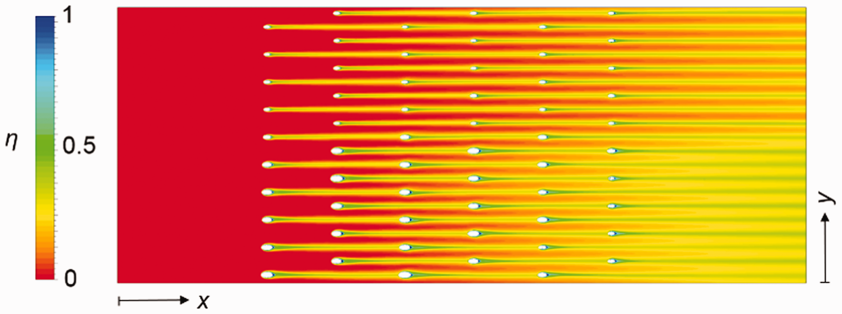

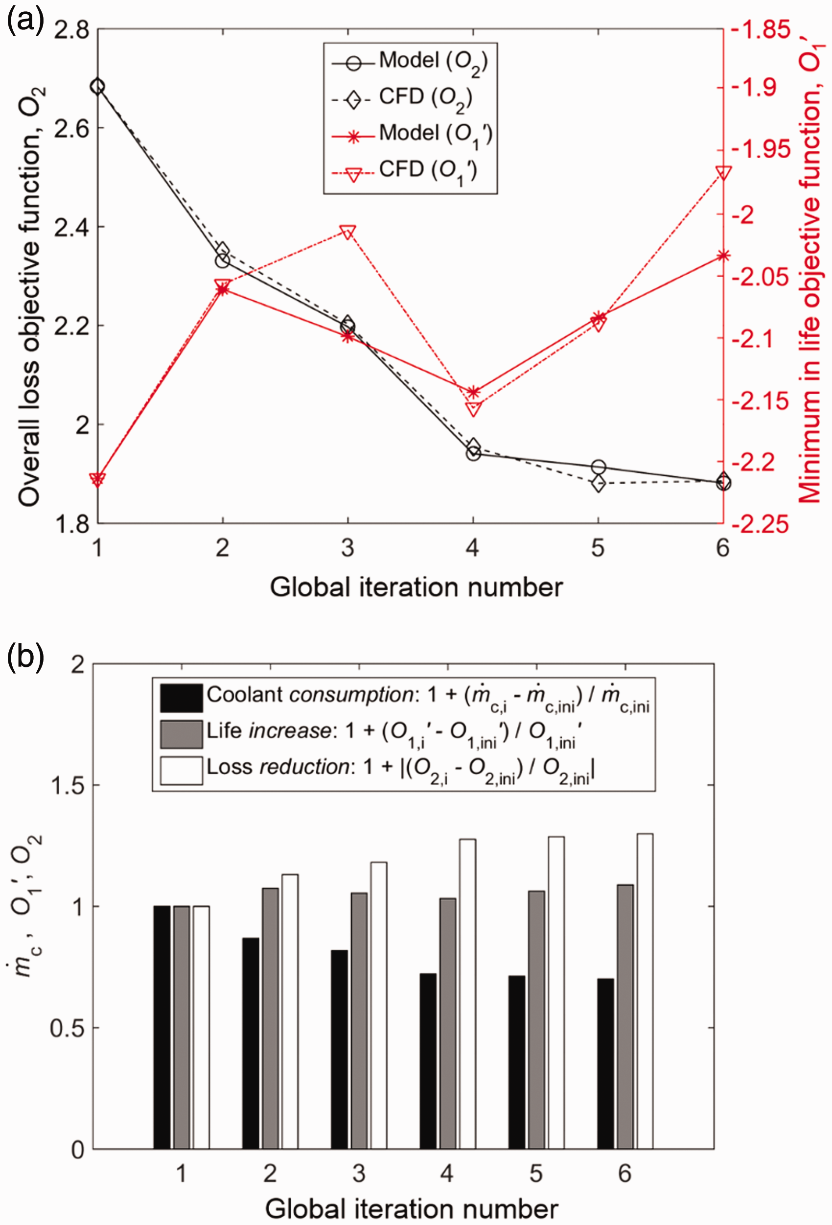
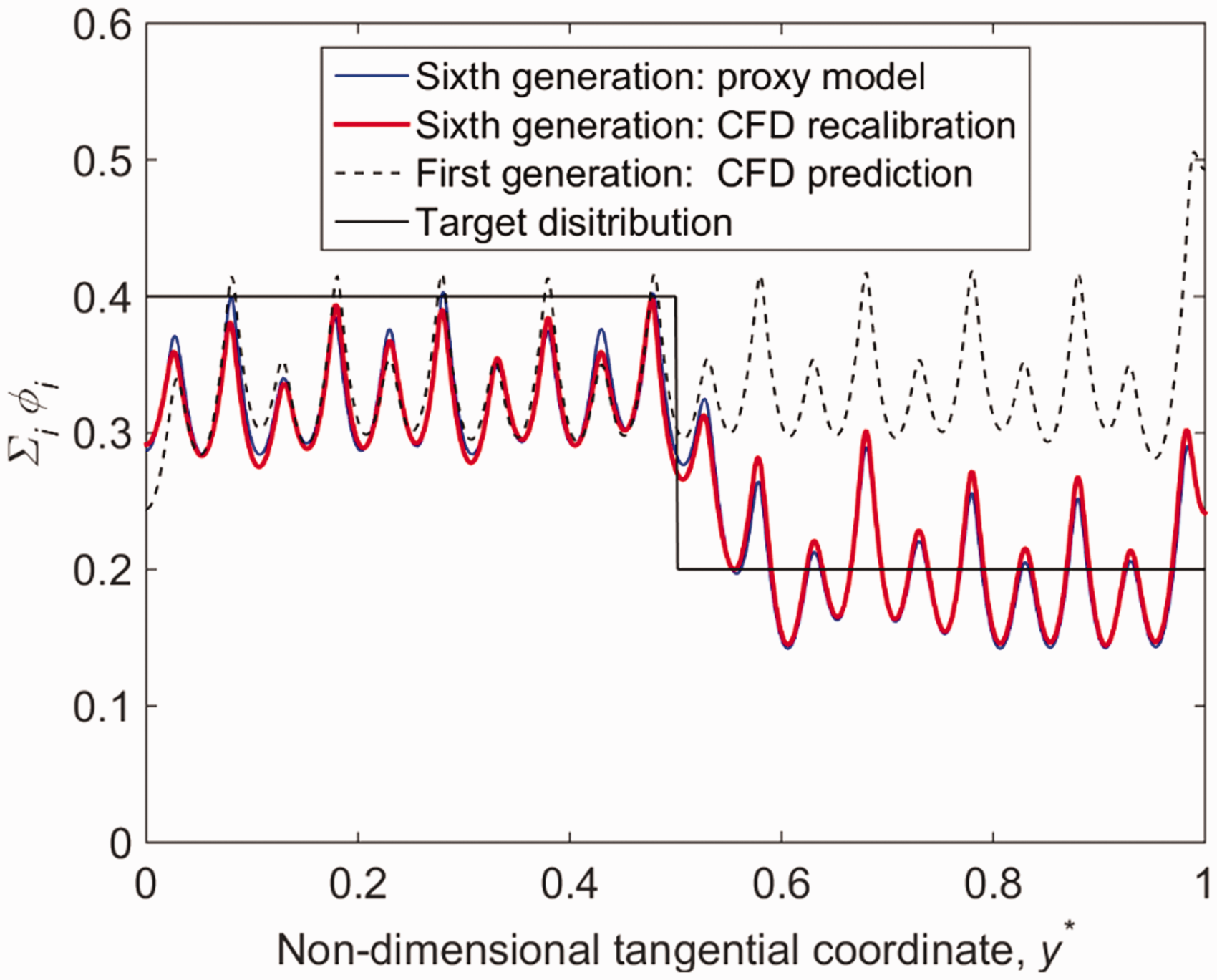
Figure 14(a) presents the evolution of the minimum in the life objective function, $O_{1}'$ , and the value of overall loss objective function, $O_{2}$ , for each global iteration of the method. CFD and model prediction results are compared.

The evolution of $O_{1}'$ shows reasonably good agreement between model and CFD predictions for each global step (recalibration step), with significant differences only at iterations 3 and 6. These differences (particularly at iteration 3, for which the CFD and model are in directional difference, i.e. different sign of change) serve as a good illustration of the limitations of the technique, which can fail at an iteration due to either sudden (with film cooling changes) flow structure changes in the main-flow or sudden local flow structure changes not included in the framework of the model. Whether or not this leads to the method failing to pass a local minimum depends on the experience of the user in application to a particular test case. These limitations are discussed more extensively in the following section.

The evolution of $O_{2}$ shows very good agreement between model and CFD predictions for all global step (recalibration step), with no significant differences between model and CFD. At each global step there is a reduction in the loss objective function, with evidence of an asymptote being reached at global iterations 4 and 5. It is worth noting that the worsening (decrease) in the minimum of the life objective function ( $O_{1}'$ ) at global iteration 4 is accompanied by a significant improvement (decrease) in the loss objective function ( $O_{2}$ ) at the same global iteration number. Whether or not both functions need to be improved at every step depends on the method of picking the ‘fittest’ solution from the Pareto front. In our case this was done manually, by picking a point approximately in the middle of the front.

In Figure 14(b) we show the evolution of coolant consumption, life, and loss reduction as a function of the global iteration number. The optimization process was stopped after six global iterations because the improvement in both objective functions between two subsequent global iterations was small (less than 3%) showing a plateau in the optimization. After six global iterations of the optimization process, the minimum in the life objective function, $O_{1}'$ , was improved by 11%; the overall loss objective function, $O_{2}$ , was reduced by 30%; and the coolant mass flow was reduced by 30%. These are very significant improvements for a relatively complex multi-objective optimization and show the power of the proposed method.

In summary, the proposed method has achieved convergence to an optimized configuration after only six CFD simulations. This is a reduction in computational cost of several orders of magnitude over standard methods. Both objective functions ( $O_{1}'$ and $O_{2}$ ) were substantially improved with respect to the initial configuration.

Further discussion of results

We now consider in more detail the evolution of the objective functions during the optimization process.

In Figure 15 we compare the target film effectiveness distribution (solid black line) at the domain exit ( $x / d =$ 35 from the last row of holes), the film effectiveness distribution for the first generation design (dotted black line), and the proxy model output (blue line) and CFD recalibration prediction (red line) for the sixth generation design. We recall that the target function was chosen as an arbitrary (but somewhat complex) distribution to demonstrate the capability of the method. CFD predicted curves (red and dotted black lines) use the standard definition of adiabatic film effectiveness (equation (9)), but the model-predicted curve (blue line) is calculated as the sum of all passive scalar values.

The first generation design (dotted black line) has CFD predicted film effectiveness in the range 0.25 $< η <$ 0.5. This is lower than the target distribution in the region $0 \leq y^{*} \leq 0.5$ and higher in the region 0.5 $< y^{*} \leq$ 1.0. The highest value of film effectiveness (approximately $η =$ 0.5) is reached at approximately $y^{*} =$ 1.0 and lowest value (approximately $η =$ 0.24) at $y^{*} =$ 0.0.

After six global runs (approximately 125,000 MOGA/proxy model solutions, but only six CFD solutions) the difference between the CFD-predicted distribution and the target distribution is substantially reduced. We also see that the MOGA/proxy model estimation is in excellent agreement with the corresponding CFD prediction (comparison of red and blue lines in Figure 15).

We now consider the change between the initial and final cooling configurations when compared to the target profile. In the region $y^{*} \geq$ 0.5, we observe two main improvements (between first and sixth generation designs) in the match to the target profile. First, the global difference in film effectiveness from the target distribution is substantially reduced. In this particular case, our overcooled region is removed (this arises because of the cost associated with mixing loss). Second, the maximum peak in film effectiveness is significantly reduced (from $η =$ 0.5 to $η =$ 0.25).

In the region $y^{*} <$ 0.5, there is a relatively small change between the initial (first generation) and final (sixth generation) film effectiveness distributions. The minimum film effectiveness (at approximately $y^{*} =$ 0.0) is increased very slightly from $η =$ 0.24 to $η =$ 0.30, removing the minimum in component life, which is heavily penalized. What is interesting is that the global level of film effectiveness is not improved from the initial distribution (i.e. the difference from the target function could not be reduced). This is believed to be an artefact of the CFD process, arising from the fact that in the relatively mixed-out downstream state, quite large increases in mass flow rate have a small impact on the mixed-out film effectiveness. We will show below that the MOGA process has been very active in adjusting hole sizes (and associated mass flow rates) in the range $y^{*} <$ 0.5, but in the trade-off between the two objective functions – also taking account of the ‘best design’ selection process on the Pareto front – could not improve the film effectiveness due to the extremely low exchange rate with mass flow rate. We see that loss associated with the holes in the range $y^{*} <$ 0.5 is substantially improved though, demonstrating activity of the MOGA script towards the targets.

Figure 16 shows the evolution of $O_{1}'$ , the minimum value of the life objective at the evaluation line, in the regions 0.0 $\leq y^{*} <$ 0.5 and 0.5 $\leq y^{*} \leq$ 1.0, with global iteration number. This value is one part of the overall objective function or one axis of the domain for the Pareto front. The figure indicates activity of the optimizer in both halves of the domain.

Figure 16.

Evolution of 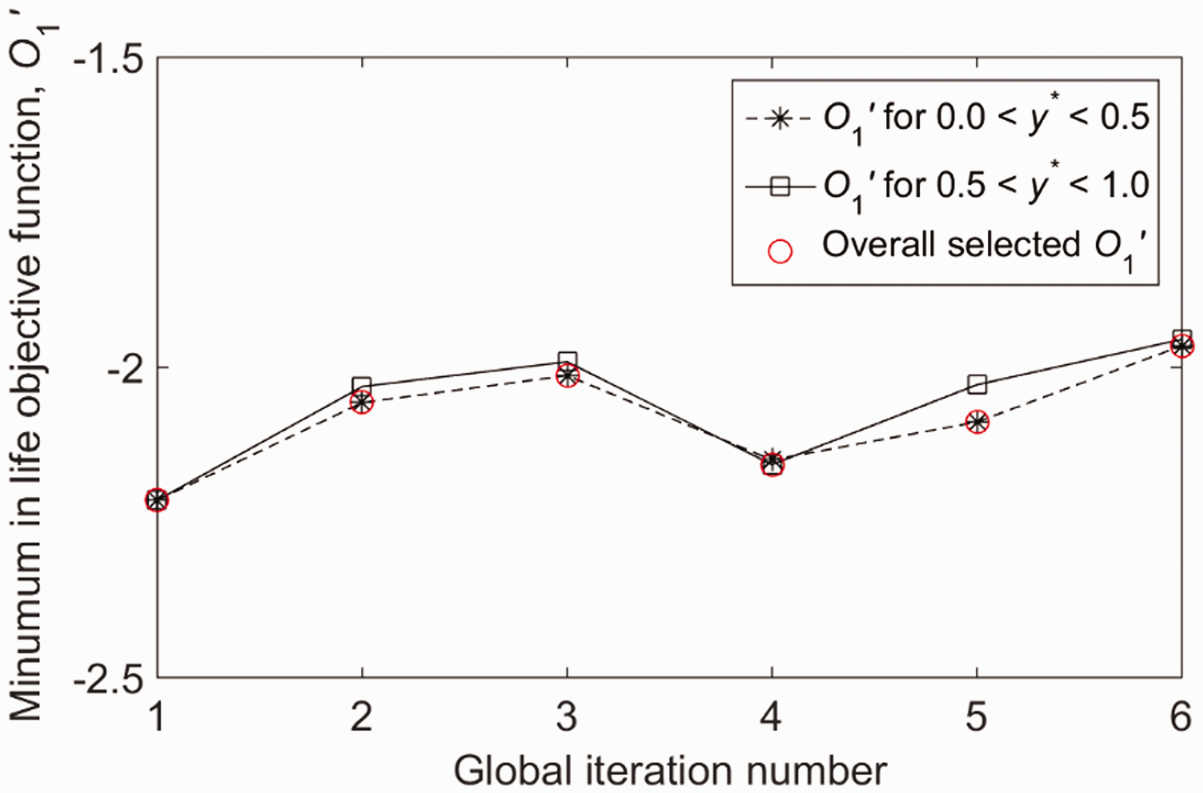$O_{1}'$ , the minimum value of the life objective at the evaluation line, with global iteration number, for the regions 0.0 $\leq y^{*} <$ 0.5 and 0.5 $\leq y^{*} \leq$ 1.0.

We now consider mixing loss, and compare the first generation and sixth generation designs. The target is to minimize overall loss (as measured by entropy gain).

Figure 17 shows the change in hole diameter for each row (individual figures) for global iterations from the first generation (d = 2 mm) to the sixth generation design. The optimized configuration is characterized by larger diameters for combinations with low row and column number (bottom left quadrant of domain shown in Figures 5 and 13, i.e. 0 < $x / d$ < 62.5 and 0 < $y / d$ < 25) and smaller diameters elsewhere in the domain (the remaining three quadrants).

Figure 17.

Evolution of hole diameters with global iteration number.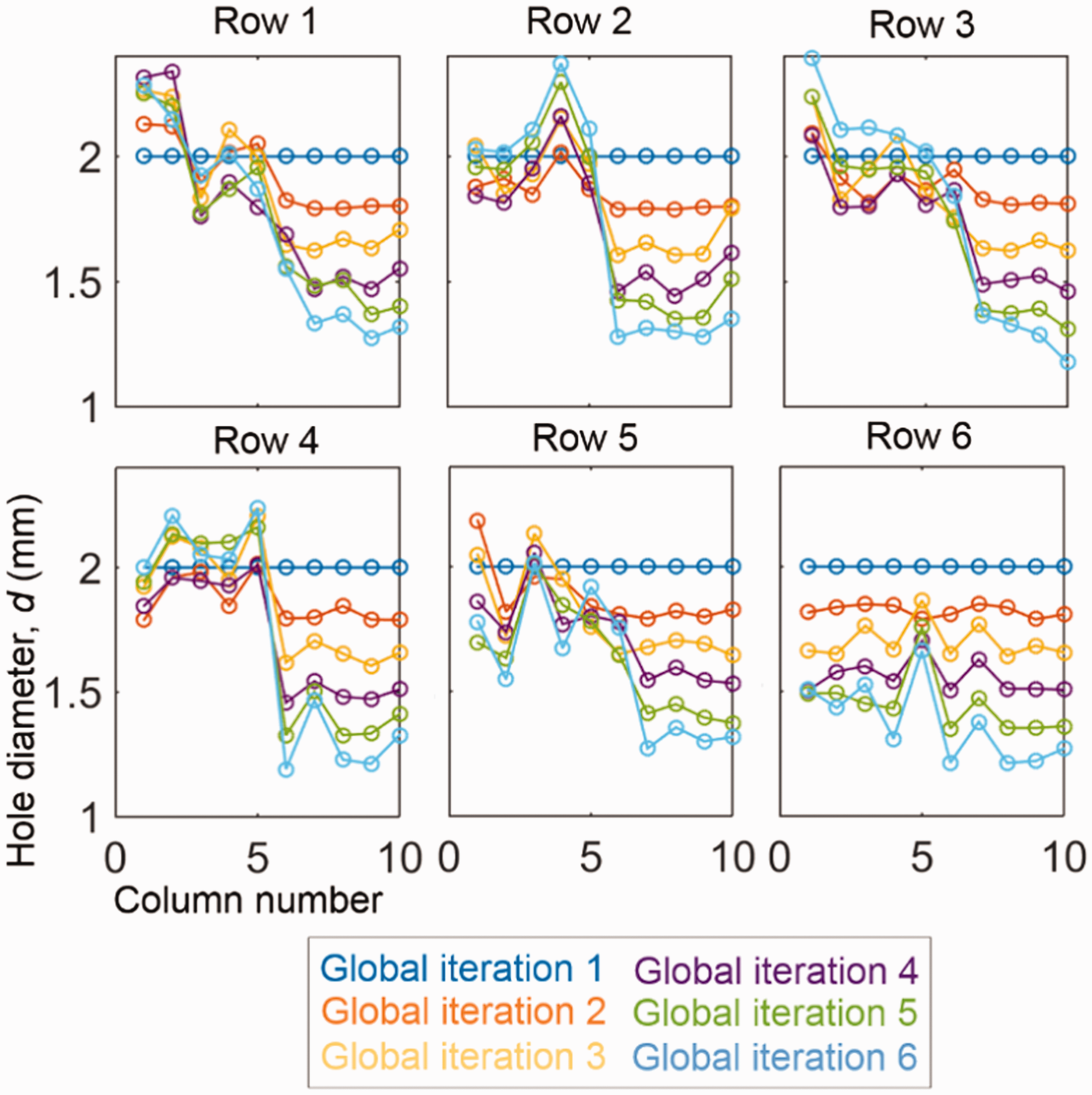

In the final optimized solution, with very few exceptions, hole diameter in a particular row decreases monotonically in the direction of the domain exit. This is because mixing loss is lower in the region of lower external Mach number. Even in this simple scenario, complexity emerges because of the coupled nature of the optimization (film effectiveness and loss).

Figure 18 shows the area distribution for all the holes for the final optimized design (solid bars, after the sixth global iteration) compared to the initial hole areas (transparent bars). Hole areas in columns 5–10 are reduced, this result being driven by the step in the target distribution of equation (12). Likewise the area of the holes belonging to rows 4–6 is reduced because of the higher mixing losses associated with injection of films into a higher Mach number region. In contrast, there is an increase in the hole area in rows 1–4 for columns 1–4.

Figure 18.

Comparison of hole areas between the initial case and the final optimized design (after given global iterations).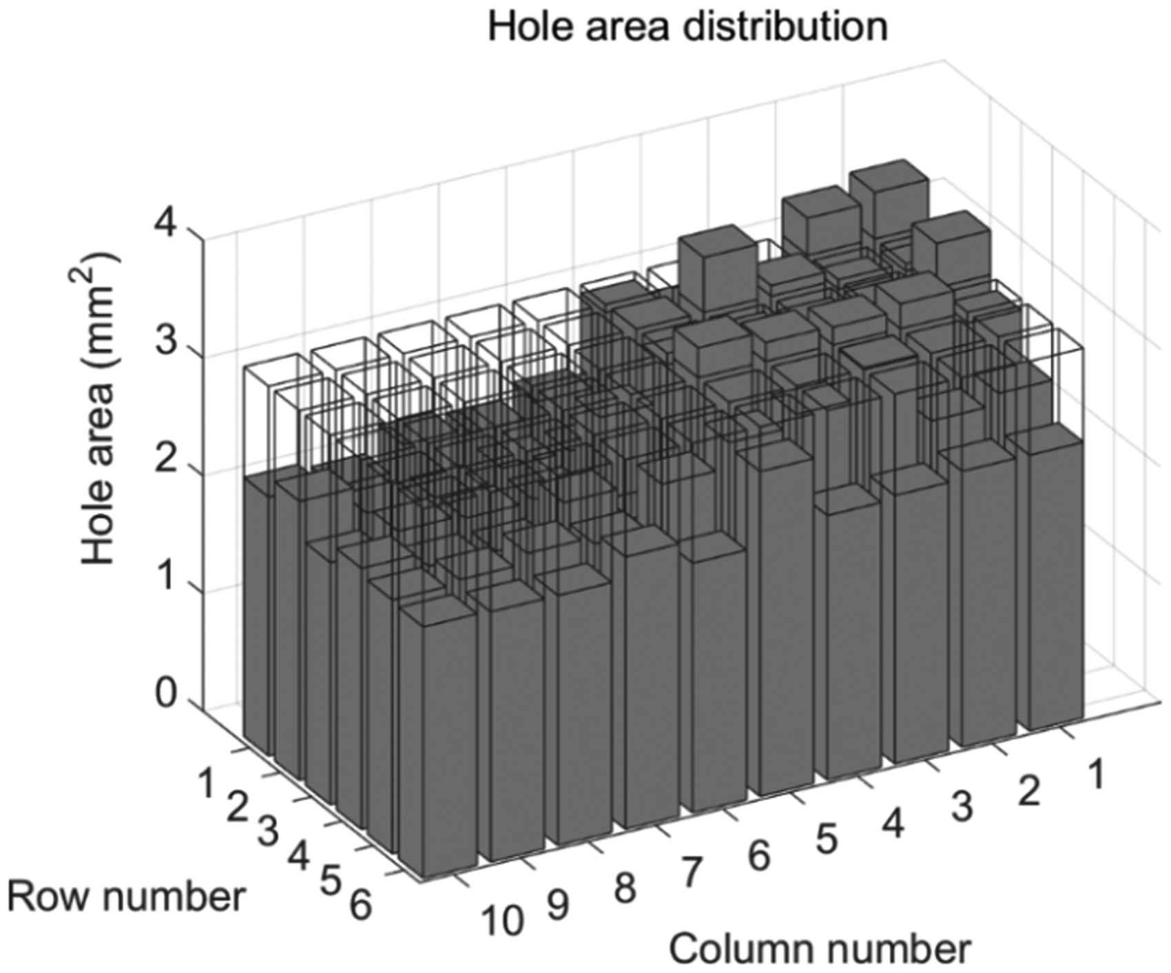

Summary of results and findings

In this paper, we have demonstrated that, with the proposed methodology, convergence of a multi-objective optimization process can be obtained with only six outer-loop iterations (six CFD simulations). This is at least two orders of magnitude less than required with standard optimization techniques and is achieved by supplementing the CFD with a proxy model which runs 10,000 computationally inexpensive inner-loop iterations per outer-loop iteration. Because the proxy model is recalibrated at each outer-loop iteration, and because the final result is validated with the outer-loop iteration, the final solution is as robust as the method used. The outer loop could be high-fidelity CFD or even an experimental technique.

The optimized solution improved on the baseline design as follows: an 11% increase in component life, a 30% reduction in overall mixing loss, and a 30% reduction in mass flow rate. The situation chosen was relatively complex, on account of the multi-objective nature of the optimization.

In the following section, we discuss limitations of the proposed method.

Limitations of the method

We have demonstrated a powerful method for optimization of film cooling systems, which reduces by more than an order of magnitude the number of CFD simulations required, replacing them with a low-order proxy model of the cooling system, seeded with information from an initial CFD simulation and periodically recalibrated against subsequent CFD simulations. Although the method is powerful, it relies on directional stability of the proxy model. By this we mean that the each time and extrapolation is performed by the proxy model, the change from the previous iteration should at least be in the same direction as the change in the higher order model of the system (in this case the CFD simulation, but, equally, we could apply the argument to an experimental system) but ideally also of the same order of magnitude. If the proxy model does not predict at least the correct direction in the change of the objective function between iterations (e.g. it predicts an improvement, but the CFD recalibration step predicts degradation), the model is unstable and convergence cannot be achieved.

In this section we discuss possible limitations of the proxy model, which would limit application of the overall method. The following possible limitations have been identified:

Sudden (with film cooling changes) flow structure changes in the main-flow. It is well-known that bulk momentum flux contribution of a cooling flow can affect the overall flow structure in the near wall region. A well-known example of this is that the film cooling flow on a nozzle guide vane platform can completely change the secondary flow structure in the passage (see, e.g. Thomas and Povey⁶ and Ornano and Povey¹⁴). The effect (with changing film cooling flow) can be so significant that regime shifts are introduced. A regime shift could be as dramatic as the sudden and complete suppressing of a passage-scale secondary flow structure. A similar effect is observed on rotor endwalls with changes in the cavity purge flow.¹⁵ The proxy model discussed in this paper does not model the dynamics of the endwall flow in a way that could capture regime shifts. If applied in environments of this type, it is possible that a local optimum could be found on one side or the other of a regime interface (defined by a particular value of coolant momentum introduction, for example), but it would be impossible for the model to extrapolate (in either direction) meaningfully through the regime change (though a solution might cross a regime by accident). In turbine cooling applications, flow structure changes at particular values of film cooling flow are surprisingly common: in such environments the combined scalar tracking, CFD, and MOGA method must be applied carefully, ideally with prior knowledge of the regimes that exist for a particular application.

Sudden local flow structure changes. It is well-known that the local momentum flux ratio (coolant-to-mainstream) affects the local state of the cooling jets (attached or separated, for example) and therefore the local flow structure. This can be quite 3D in nature, with complex interaction between the horseshoe vortex formed by the mainstream and counter-rotating vortex pair issuing from the hole. The coolant-to-mainstream momentum flux ratio affects the coolant trajectory in general (even a long way from the hole), and therefore has a significant bearing on the downstream film effectiveness. In certain environments there can be sudden changes in flow structure (with hole mass flow rate), for example the sudden detaching of a coolant jet at a critical value of coolant-to-mainstream momentum flux ratio. Such effects are not modelled in the simple proxy model used in this paper, and careful consideration needs to be given to the stability of the overall method across local regime changes for individual holes.

Conclusions

In this paper, we have demonstrated a method for significantly accelerating optimization of film cooling systems based on a combined scalar tracking method and MOGA optimization strategy. The method reduces by several orders of magnitude the number of CFD simulations required to achieve a converged solution. An example is discussed in which several tens of thousands of simulations are replaced with six simulations.

In the method, the CFD solution is first used to predict the flow domain for the film cooling system. Scalar tracking is implemented in the CFD to identify the contributions of individual holes to an overall cooling effectiveness distribution (this is done by associating a unique passive scalar variable to the flow associated with each hole and solving an additional scalar transport equation). A proxy model of the CFD solution (simple superposition model, taking scalar values from the CFD solution) is then used to extrapolate to new design points using the MOGA method, targeting improvement against a defined objective function (which might include coolant consumption, life, and loss). The process works as an inner (proxy model) and outer (high-fidelity CFD) convergence loop. The outer loop is used to periodically recalibrate the proxy model in the inner loop to prevent divergence.

We demonstrate that convergence for a complex objective function can typically be achieved with six outer-loop iterations (high-fidelity CFD runs) and 10,000 inner-loop iterations per outer-loop iteration. Our example had an objective function which maximized the component life and minimized the mixing loss introduced by the films. A 30% reduction in mixing loss, a 11% increase in component life, and a 30% reduction in cooling mass flow rate were achieved.

There are some limitations of the proposed method which have been discussed. Particular care needs to be taken when there might be either sudden changes (with changing film cooling flow rate) in the main-flow structure (e.g. suppression or enhancement of a secondary flow) caused by a change in cooling flow or sudden changes in the local flow structures (e.g. jet detachment) caused by the same. In these situations, a simple proxy model would not be able to extrapolate (in either direction) meaningfully through the regime change. This can be mitigated by a user who understands the sensitivities for the part being optimized.

The significant advantage of the proposed method is that for certain optimization problems, the computational cost can be reduced by several orders of magnitude, replacing thousands of high-fidelity CFD runs with approximately six CFD runs. In principle, the technique is applicable to other optimization processes, in which, for example, the high-fidelity CFD simulations are replaced by experiments.

Footnotes

Declaration of Conflicting Interests

The author(s) declared no potential conflicts of interest with respect to the research, authorship, and/or publication of this article.

Funding

The author(s) received no financial support for the research, authorship, and/or publication of this article.

ORCID iD

Thomas Povey

References

Ayoub CE. Three-dimensional aero-thermal optimization of film cooling in a high pressure turbine. PhD Thesis, Concordia University, Canada, 2014.

Jiang

Lin

Yue

, et al. Aero-thermal optimization on multi-rows film cooling of a realistic marine high pressure turbine vane. Appl Therm Eng 2017; 111: 537–549.

Johnson

King

Clark

, et al. Genetic algorithm optimization of a high-pressure vane pressure side film cooling array. ASME J Turbomach 2014; 136: 011011, pp.1–11 .

Thomas M. Optimization of endwall film-cooling in axial turbines, PhD Thesis, University of Oxford, UK, 2014.

Thomas M, Kirollos B, Jackson D, et al. Experimental and CFD studies of NGV endwall cooling. In: Proceeding of the ASME Turbo Expo 2013: turbine technical conference and exposition, San Antonio, Texas, USA, 3–7 June 2013, paper no. GT-2013-95636.

Thomas

Povey

. A novel scalar tracking method for optimising film cooling systems. Proc IMechE, Part A: J Power and Energy 2013; 230: 3–15.

Hartsel JE. Prediction of effects of mass-transfer cooling on the blade-row efficiency of turbine airfoils. In: AIAA 10th aerospace sciences meeting, San Diego, CA, 17–19 January 1972, AIAA paper no. 72-11.

Kollen O and Koschel W. Effect of film-cooling on the aerodynamic performance of a turbine cascade. In: AGARD CP-390, 1985, pp.1–16.

Young

Wilcock

. Modeling the air-cooled gas turbine: part 2 – coolant flows and losses. ASME J Turbomach 2002; 124: 214–221.

10.

Adams BM, Ebeida MS, Elred MS, et al. Dakota, a multilevel parallel object-oriented framework for design optimization, parameter estimation, uncertainty quantification, and sensitivity analysis: version 6.2, user manual. SAND2014-4633. Albuquerque, NM: Sandia National Laboratory, 2015.

11.

Eddy J and Lewis K. Effective generation of Pareto sets using genetic programming. In: Proceedings of DETC'01, ASME 2001 design engineering technical conferences and computers and information in engineering conference, Pittsburgh, PA, 9–12 September 2001, paper no. DETC2001/DAC21094.

12.

Fonseca CM and Fleming PJ. Genetic algorithms for multi-objective optimization: formulation, discussion, and generalization, genetic algorithms. In: Proceedings of the fifth international conference, San Mateo, CA, July 1993.

13.

Sellers

. Gaseous film cooling with multiple injection. AIAA J 1963; 1: 2154–2156.

14.

Ornano

Povey

. Experimental and computational study on the effect of momentum-flux ratio on high-pressure nozzle guide vane endwall cooling systems. ASME J Turbomach 2017; 139: 121002-1–14.

15.

Cui

Tucker

. Numerical study of purge and secondary flows in a low-pressure turbine. ASME J Turbomach 2017; 139: 021007, pp.1–10.

Combined scalar tracking,computational fluid dynamics,and multi-objective genetic algorithm method to accelerate optimization of film cooling systems

Abstract

Keywords

Introduction

The scalar tracking method

Combined scalar tracking CFD and MOGA method

Defining the objective functions

Defining and initializing the proxy model with a first CFD solution

Defining the exchange rate between hole diameter and mass flow rate

Defining the effectiveness contribution for new hole locations

MOGA extrapolation of the proxy model

CFD validation of the MOGA/proxy model output

Stability check of the proxy model over a particular outer-loop iteration

Recalibration of the proxy model

Flat plate test case

General design of the flat plate test case

Defining the objective functions

CFD setup and initialization of the proxy model

Defining the exchange rate between hole diameter and mass flow rate

Details of the MOGA algorithm used in the present example

Results and discussion

General results

Further discussion of results

Summary of results and findings

Limitations of the method

Conclusions

Footnotes

Declaration of Conflicting Interests

Funding

ORCID iD

References