Sage Journals: Discover world-class research

Abstract

Resource constraints in neural information processing imply that numerical discriminability optimally adapts to the frequency of numerical magnitudes in a decision maker’s environment. Here, we tested the economic consequences of efficient numerical range adaptation in representative samples of the United Kingdom and Japan (N = 2,309) and in a replication in Austria and Hungary (N = 607). We exploited natural variation in currency units and combined it with an orthogonal variation in experimental currency units to detect the effect of habitual versus nonhabitual numerical ranges on the incidence of errors in decisions under risk. The results highlight the direct economic importance of numerical adaptation, thus calling into question standard assumptions that choice quantities are perceived without noise.

Keywords

numerical adaptation resource constraints money illusion consistency errors

Humans have adapted to living across a wide range of conditions. Given biologically imposed limits to cognitive resources (Bhui et al., 2021; S. B. Laughlin et al., 1998; Lieder & Griffiths, 2020), optimal adaptation to specific local situations will come at the cost of increased errors for decisions that fall outside the habitual range (Louie et al., 2015). This suboptimality can be organized by a resource-constrained version of Weber’s law, whereby the constraint makes adaptation to the stimuli of the environment optimal. Such optimal adaptation has long been modeled in neuroscience (Heng et al., 2020; S. Laughlin, 1981; Rustichini et al., 2017), psychology (Stewart, 2009; Stewart et al., 2006, 2014), and economics (Khaw et al., 2017, 2021; Netzer, 2009; Padoa-Schioppa, 2009; Padoa-Schioppa & Conen, 2017; Polania et al., 2019; Robson, 2001; Vieider, 2023).

All of these approaches share the intuition that people will be more likely to misrepresent numbers that fall outside of the numerical range to which they are adapted than numbers within that range. This, in turn, may lead to increased error rates outside the familiar range.¹ Studies investigating this issue have made great strides in accounting for previously unexplained paradoxes using data from laboratory experiments (Khaw et al., 2021; Vieider, 2024; Zhang et al., 2020). The economic impact of such processes outside of laboratory settings—and hence their importance in actual economic terms—has, however, received much less attention. The question of whether range adaptation affects real-world everyday economic decisions is, however, crucial if we want to consider whether to modify the standard assumption that choice quantities and their value are perceived accurately.

Here, we empirically tested the economic relevance of numerical range adaptation for real-world economic decisions. We exploited natural differences in monetary denominations across countries to conduct a field test of the economic relevance of adaptation to a specific numerical range while at the same time keeping tight experimental control, which allowed us to draw causal inferences about the drivers of behavior. This test rested on the idea that adaptation takes place with respect to numbers rather than pertaining inherently to economic value (Enke et al., 2023; Oprea, 2024; Vieider, 2024). It furthermore builds on a large literature showing how number perception may be influenced by the specific numerical range to which a decision maker is habituated (Khaw et al., 2021; Piazza et al., 2004; Prat-Carrabin & Woodford,. 2022).

In some countries the range of prices people are exposed to on a regular basis (e.g., while shopping, in advertisements) is between one and three digits (e.g., the euro in many European countries, U.S. dollars, or British pounds). In other countries, however, equivalent purchases require numbers between five and seven digits (e.g., the Hungarian forint, Czech koruna, or Japanese yen). We hypothesized that people in specific countries would be better at making economically relevant decisions in the numerical currency range with which they were familiar compared with when the involved monetary amounts fell outside of their habitual range. In particular, we expected decisions falling outside of the usual currency range to be subject to more frequent and larger mistakes, which may lead to monetary losses. People accustomed to small numerical currency ranges would thus be particularly liable to make mistakes with large numbers, whereas people habituated to large numerical values would be more liable to make mistakes with small numbers. The use of natural monetary units, in turn, ensured high external validity of our results.

To allow for causal inferences to be drawn, we combined the naturally occurring variation between countries with experimentally induced variation within countries. In particular, we compared a small-denomination currency (British pounds) to a large-denomination currency (Japanese yen), where all monetary pound amounts were multiplied by a factor of 180.² To minimize confounds deriving from economic or cultural differences, we based our tests on a symmetric setup in which participants in both countries faced both large and small numerical payoffs. The hypothesis entailed that subjects in the United Kingdom would make more mistakes for payoffs denominated in large numerosities (i.e., when scaling up all payoffs 180-fold while keeping the underlying economic value constant). Conversely, we predicted that Japanese participants would make a larger number of mistakes for payoffs denominated using small numerosities (i.e., when dividing the numerical units in which a given economic value is represented by 180). To isolate the numerical effect of currency units, we conducted the experiments in both countries using identical “experimental currency units” that could correspond either to the national currency one to one or have a conversion rate to map it into denominations typical for the other country (multiplying by 180 in the United Kingdom and dividing by 180 in Japan) while keeping the actual economic value of the choices constant. We chose the monetary payoffs and conversion rates so that all outcomes could be expressed using integers to eliminate any potential confounds that could be derived from the use of decimals.

We relied on lottery choices for our tests. We chose decisions under risk both for their economic relevance and because they had been used in recent publications on this topic (e.g., Frydman & Jin, 2022; Garcia et al., 2023; Khaw et al., 2021; Vieider, 2023; Webb et al., 2020). Traditionally, choices under risk have been modeled by assuming that people’s behavior can be characterized by means of stable preferences (Kahneman & Tversky, 1979; von Neumann & Morgenstern, 1944). Such as-if explanations, however, cannot account for evidence that individuals’ risk taking propensity may systematically adapt to the environment faced by the decision maker (Cohn et al., 2015; Di Falco & Vieider, 2022). They have also been criticized for making arbitrary assumptions about the origin of noise (Alós-Ferrer et al., 2021). Lottery choices were well suited for the tests we proposed because we could leverage dominance relationships between lotteries to measure error rates even in a subjective, preferential context. The use of choice under risk further allowed us to quantify the “cost” of numerical range adaptation (i.e., how much money people stood to lose). We further used representative samples of the countries to enhance the external validity of the results.

Note that any results of our manipulation could not possibly be explained away by “calculation difficulties.” In particular, any such “difficulties” are a manifestation of the very idea of approximate numerical judgments being aided by the adaptation we aimed to study. The only principle that subjects need to follow in our setting to avoid errors is “more is better,” which ought to be independent of the numerical magnitudes. The asymmetry in our design furthermore ensured that smaller numbers (or, for that matter, larger numbers) being generally easier to process and compare also could not possibly account for our findings.

Our study explicitly captured and tested predictions from several related models. One caveat with this approach is that it tested the range-adaptation hypothesis at large rather than testing a specific model. Given that the details of the predictions could depend on fine-grained modeling assumptions, our tests were ill suited to discriminate between different models within the adaptive class. A second caveat concerns the speed of adaptation. Although a large variety of models make predictions about optimal adaptation, very few of them incorporate specific dynamic equations. We chose to see this as an opportunity. In particular, we partitioned the time sequence of tasks into subsets of 40 tasks and separately tested the quantities of interest for these subsets. If adaptation is fast, we would expect the predicted patterns to occur in early batches of tasks but to vanish over the course of the experiment. This testing sequence thus allowed our experiments to be informative for future modeling exercises aiming to capture the speed of adaptation.

The numerical range adaptation hypothesis we tested may be considered optimal subject to resource constraints. That is, given inherent constraints in neural processing, adaptation typically abides by some principle of constrained optimization. Given the quick variability of numerical magnitudes in the modern world, this could nevertheless result in costly mistakes while traveling or trading in assets denominated in foreign currencies. Cryptocurrencies, online casinos, and video games typically entail very different numerical values than the currency denominations people are used to. People may then fall prey to “money illusion” (Shafir et al., 1997). Money illusion has been shown not only to bias individuals’ decisions but may also have profound economic consequences in the aggregate (Fehr & Tyran, 2001, 2007). Hence, this study also sought to identify the underlying mechanism leading to money illusion and explain the mixed empirical results found in the literature (e.g., Desmet, 2002; Gamble et al., 2002; Raghubir & Srivastava, 2002). The hypothesis we tested further has implications for the design of experiments. Experimental currency units are often used to give the illusion of larger stakes, with the aim of increasing attention and rationality. Numerical range adaptation, however, suggests that such procedures could have the exact opposite effect because they may actually increase error rates rather than reducing them.

Research Transparency Statement

General disclosures

Conflicts of interest: All authors declare no conflicts of interest. Funding: This research was supported by departmental funds from the University of Ghent and by Research Foundation–Flanders Grant G008021N. Artificial intelligence: No AI-assisted technologies were used in this research or the creation of this article. Ethics: This research complies with the Declaration of Helsinki (2023), and the study was approved by the University of Ghent Faculty of Economics Ethical Commission (UG-EB 2023-I). Open Science Framework: A registered version of the OSF project is available at https://osf.io/wfzhn/files/osfstorage.

Study 1 disclosures

Preregistration: The research hypotheses, methods, and analysis plan were preregistered at https://osf.io/r76gt on November 14, 2023, prior to data collection, which began on November 17, 2023. Note that although this was not a formal OSF preregistration, the journal’s STAR team has used the OSF time stamp to confirm that the linked file has not been modified and therefore would suffice as a preregistration. There were minor deviations from the preregistration that were requested by the editor or the referees. In particular, the analysis of earnings differences across conditions in the “Results” section was not preregistered. Participants’ numeracy skills (Lipkus et al., 2001) were elicited but not analyzed. Materials: All study materials are publicly available at https://osf.io/fqzku under the BSD 2-Clause Simplified License. Data: All primary data are publicly available at https://osf.io/p6u9a. Analysis scripts: All analysis scripts are publicly available at https://osf.io/54rhe. Computational reproducibility: The computational reproducibility of the results has been independently confirmed by the journal’s STAR team.

Study 2 disclosures

Preregistration: The replication study was performed on request of reviewers and was not preregistered. Materials: All study materials are publicly available at https://osf.io/9yexu under the BSD 2-Clause Simplified License. Data: All primary data are publicly available at https://osf.io/p2nx6. Analysis scripts: All analysis scripts are publicly available at https://osf.io/3j6bu. Computational reproducibility: The computational reproducibility of the results has been independently confirmed by the journal’s STAR team.

Study 1: Primary Study in the United Kingdom and Japan

Method

We recruited a representative sample according to geographical location, age, gender, and income of 2,309 participants (1,157 respondents from the United Kingdom and 1,152 respondents from Japan) through Bilendi, a company providing representative subject pools for survey and experimental studies. The Japanese instructions were translated from the original English. We then had the instructions back-translated into English, and discrepancies were eliminated in discussions to arrive at the final version of the instructions. This research complies with the Declaration of Helsinki (2023), and the study was approved by the University of Ghent Faculty of Economics Ethical Commission (UG-EB 2023-I).

For each country, half of the participants were randomly assigned to the “low” condition, and the other half were assigned to the “high” condition. Participants took about 15 min to complete the study. The study was preregistered on OSF.³ Participants who failed the attention check at the beginning of the study and those who did not complete the study were excluded from the required sample size. We collected data until a sample size of at least 1,136 participants for each country was reached (for a total of at least 2,272 participants). The sample size was determined by a power calculation to guarantee an a priori power of .95 for a nonparametric, between-subjects Mann-Whitney test, small effect size, and one-tailed distribution.⁴ This sample size was also sufficient to guarantee that the Bayes factor (BF) would be at least 10 times in favor of the experimental hypothesis over the null hypothesis, starting from an uninformative prior. Participants were blind to the aim of the study and the condition they were in.

At the beginning of the study participants were informed about the general nature of the study, and we collected their informed consent to participate. They were also informed that their data would be treated completely anonymously and that they could leave the study at any moment in case they wanted to withdraw their consent. They then received more detailed instructions informing them about the structure of the choice problem, the payment procedures, and the exchange rate between the experimental currency units in which outcomes were represented. After being presented with the complete instructions and some examples of the choice tasks, participants needed to pass a simple attention check. Participants who did not pass the attention check could not continue the study and were hence excluded from the analysis.

The main part of the study required participants to make 160 binary lottery choices (for the complete list of lotteries, see the Supplemental Material available online). Figure 1 depicts the structure of the experiment.⁵ Every participant saw the same lotteries. The lotteries were constructed from 16 ordered sequences but were presented to participants as forced binary choices in randomized order. The binary choices involved a comparison between lotteries from List A (or List B) and those from List C. The latter contained lotteries that involved only sure outcomes (probabilities of 100% to get a certain amount of money). Lotteries belonging to List A or List B, on the other hand, had different probabilities across the different sequences but the same probability within the same sequence. For a given position in the ordered sequence, lotteries belonging to List B involved larger outcomes than those in List A but had the same probability. For a fixed position in the sequence lotteries in List B thus stochastically dominated lotteries in List A. For instance, take a lottery from List A, $(50 %, {Out}_{A_{i}})$ , paying ${Out}_{A_{i}}$ with probability 50%, where i from 1 to 10 indicates the position in the list. The stochastic dominance relation implies that ${Out}_{A_{i}} < O u t_{B_{i}}$ for each i; thus, (indirect) choices between such lotteries allowed us to quantify the incidence of stochastic dominance violations. For example, the first row of the list of stimuli in Tables 1 and 2 in the Supplemental Material, where i = 1, presents a lottery from List A, $(50 %, 26)$ , paying 26 European currency units (ECU) with 50% probability; a lottery from List B, $(50 %, 28)$ , paying 28 ECU with 50% probability; and a lottery from List C, $(100 %, 3)$ , paying 3 ECU with 100% probability. Because B is clearly better than A, choices of A over C are considered errors if they are not accompanied by choices of B over the same C. That is, if A is preferred to C in Row i, then B also needs to be preferred to C in that row. Likewise, if C is chosen over B, then C must be also preferred to A, and all other instances are considered errors.

Table 1.

Study 1 Random-Effect Regression of Error Rates Defined as the Number of Multiple Switches (Models 1 and 2) or the Number of Stochastic Dominance Violations (Models 3 and 4)

Error rate	Multiple switches		Stochastic dominance violations
Error rate	Model 1	Model 2	Model 3	Model 4
High	1.022*** (0.170)	0.999*** (0.171)	1.895*** (0.432)	1.975*** (0.435)
Japan	1.092*** (0.169)	1.046*** (0.177)	1.508*** (0.430)	1.352*** (0.449)
High × Japan	−2.234*** (0.241)	−2.192*** (0.245)	−4.468*** (0.611)	−4.630*** (0.622)
Age		−0.000 (0.004)		0.042*** (0.010)
Females		0.005 (0.125)		0.027 (0.318)
Income		0.001 (0.000)		−0.001** (0.001)
Risk attitude		−0.027 (0.027)		−0.118* (0.069)
Constant	21.940*** (0.120)	22.090*** (0.305)	52.290*** (0.305)	50.860*** (0.775)
N	2,309	2,221	2,309	2,221
R ²	.0362	.0362	.0253	.0379

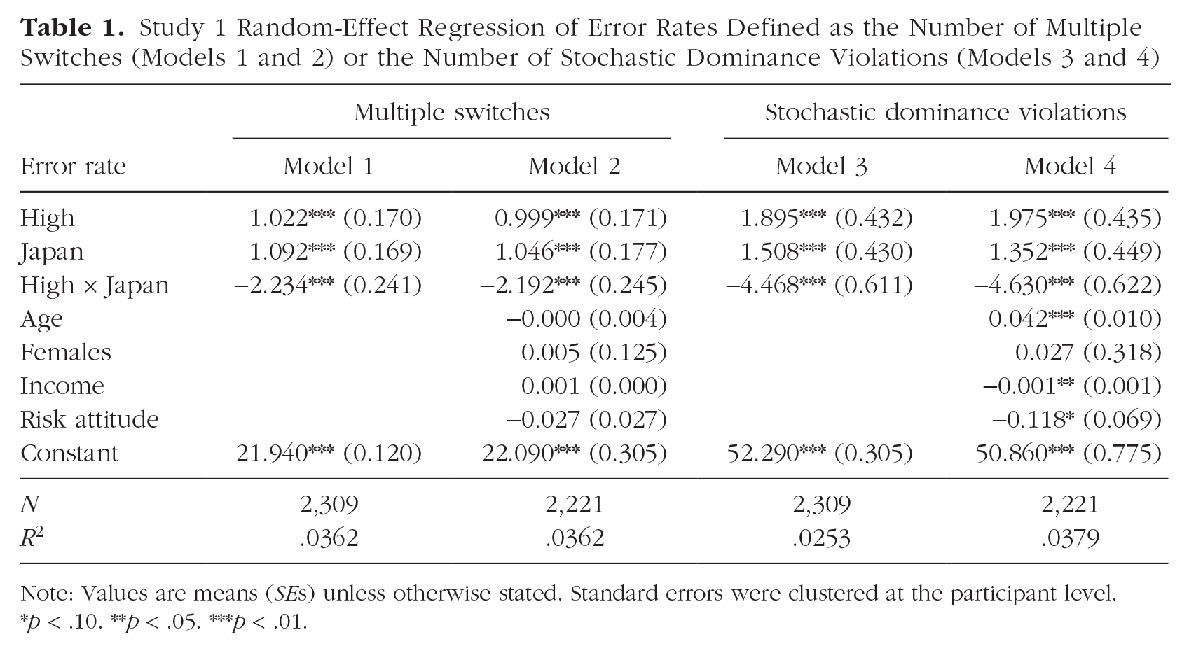
Note: Values are means (SEs) unless otherwise stated. Standard errors were clustered at the participant level. *p < .10. **p < .05. ***p < .01.

*p < .10. **p < .05. ***p < .01.

Table 2.

Study 2 Random-Effect Regression of Error Rates Defined as the Number of Multiple Switches (Models 1 and 2) or the Number of Stochastic Dominance Violations (Models 3 and 4)

Error rate	Multiple switches		Stochastic dominance violations
Error rate	Model 1	Model 2	Model 3	Model 4
High	1.930*** (0.189)	2.132*** (0.211)	2.914*** (0.622)	2.271*** (0.679)
Hungary	2.104*** (0.189)	2.176*** (0.239)	2.103*** (0.622)	1.741** (0.770)
High × Hungary	−4.367*** (0.267)	−4.545*** (0.292)	−5.953*** (0.878)	−5.262*** (0.940)
Age		−0.000 (0.010)		0.024 (0.025)
Females		0.221 (0.157)		−0.024 (0.505)
Income		0.001 (0.001)		−0.001 (0.004)
Risk attitude		−0.035 (0.035)		−0.445*** (0.114)
Constant	21.354*** (0.135)	21.334*** (0.372)	51.382*** (0.440)	53.478*** (1.197)
N	607	520	607	520
R ²	0.306	0.327	0.077	0.096

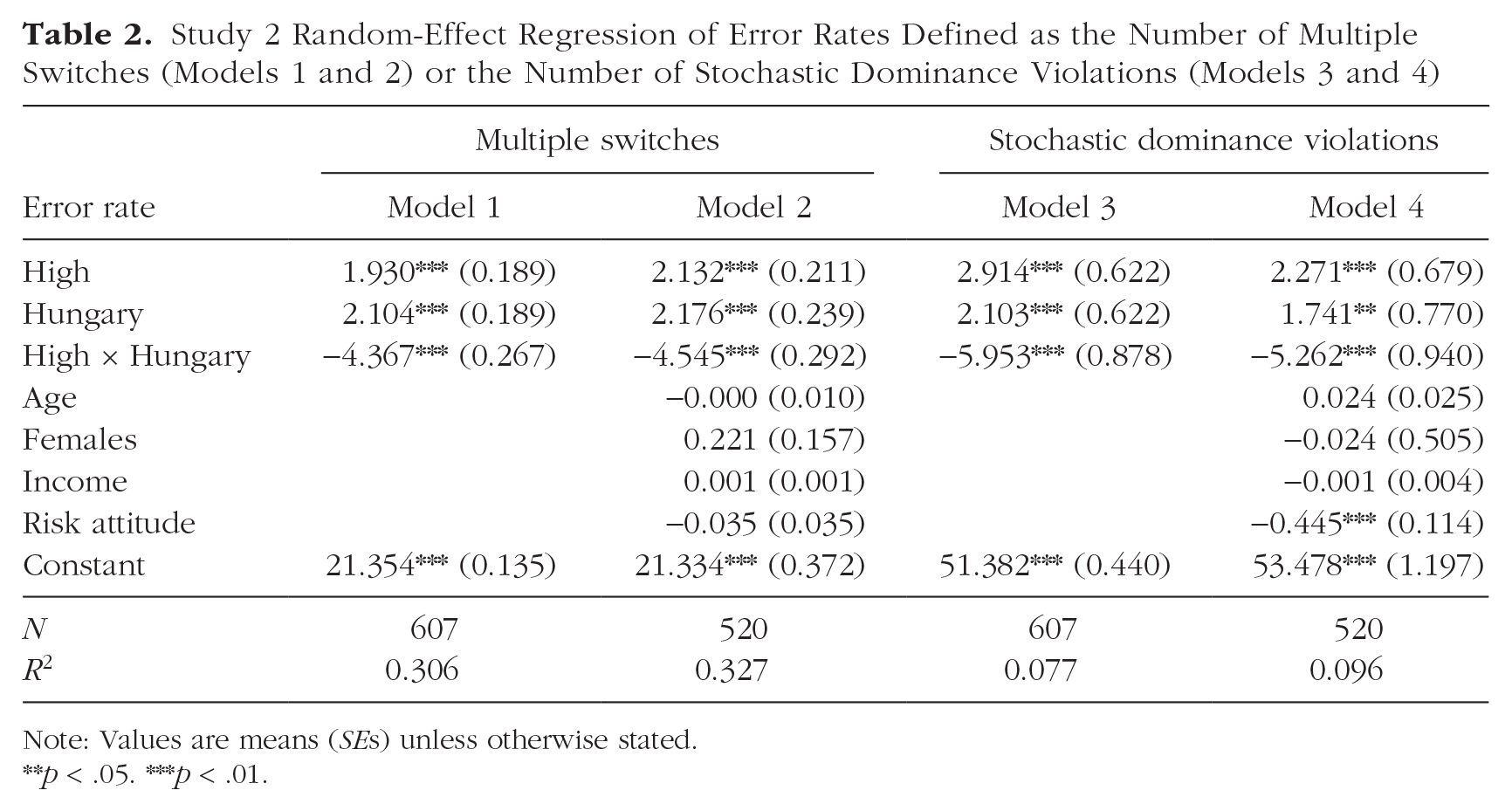
Note: Values are means (SEs) unless otherwise stated. **p < .05. ***p < .01.

**p < .05. ***p < .01.

Fig. 1.

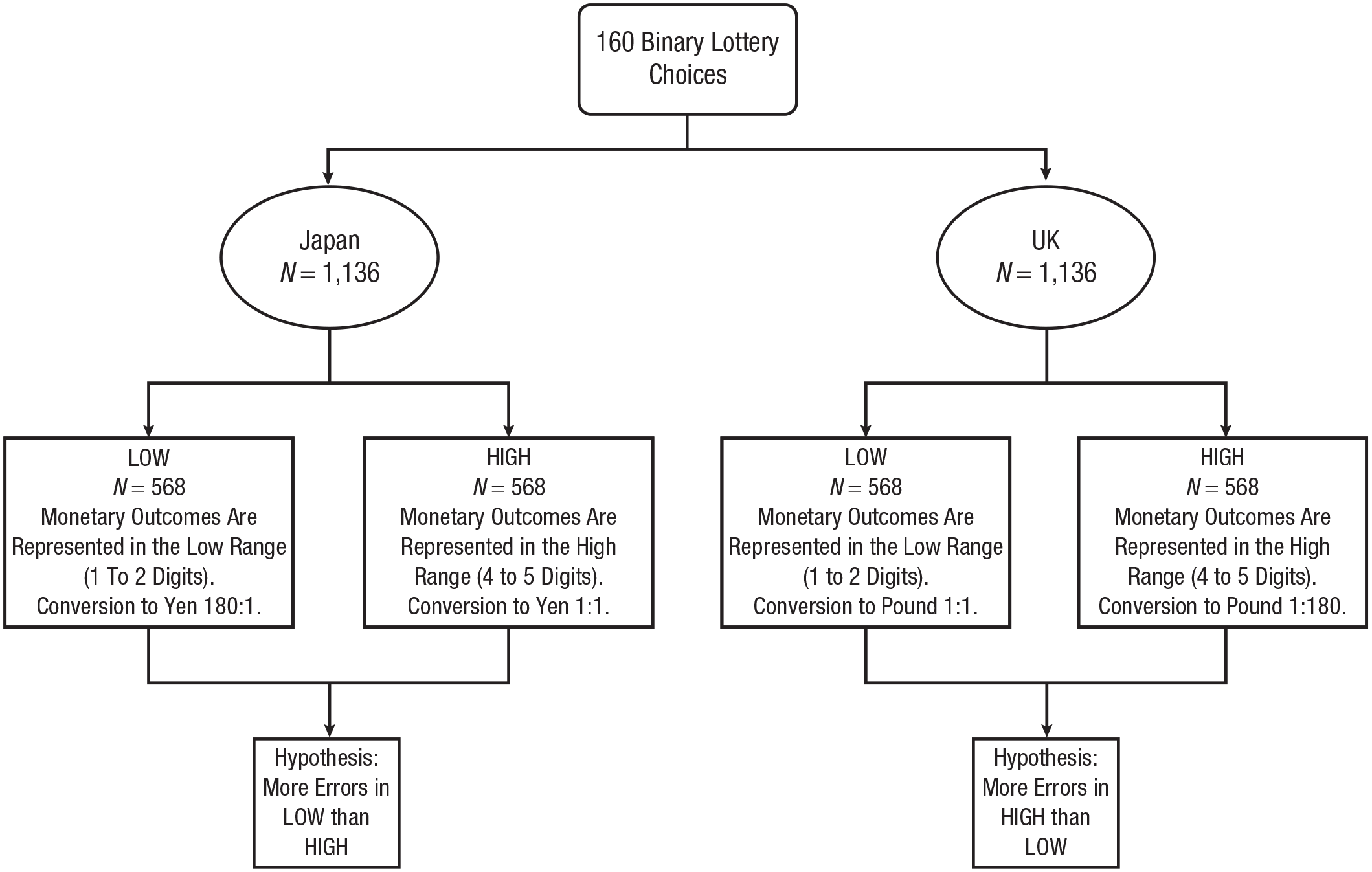
Treatment assignment flow chart. All participants saw the same set of 160 lotteries. Participants randomly assigned to the “low” groups saw the outcomes of the lotteries represented using one to two digits, whereas participants in the “high” groups saw them represented with four to five digits. We expected participants from the United Kingdom to exhibit less errors in the low range (their familiar range) than the high range. The opposite should be true for participants in Japan.

Another way in which we assessed errors was the number of inconsistent choices within an ordered sequence of 16 lotteries (e.g., Garagnani, 2023; Holt & Laury, 2002). If participants choose C_n over A_n at the nth position of the ordered sequence it implies that they should also choose C_m over A_m for all m > n because the lotteries improve systematically as one moves down the list. Inconsistencies in choice patterns are taken to be indicative of errors. For example, within the first list of stimuli in Tables 1 and 2 in the Supplemental Material, if participants choose A $(50 %, {Out}_{A_{i}} = 41)$ over C $(100 %, {Out}_{A_{i}} = 18)$ in Row 4 (n = 4) but C $(100 %, {Out}_{A_{i}} = 23)$ over A $(50 %, {Out}_{A_{i}} = 46)$ in Row 5 (n = 5), then they will also choose C $(100 %, {Out}_{A_{i}} = 28)$ over A $(50 %, {Out}_{A_{i}} = 51)$ in Row 6 (n = 6) and for all subsequent rows. Given the construction of the lists of lotteries, the errors we can infer from participants’ choices ought to be independent of their risk attitudes. In particular, on the basis of economic principles of rationality, everyone should avoid choosing dominated options (lotteries that give lower outcomes with the same probability). In sum, avoiding errors in our setting required no explicit calculation but only abiding by the standard principle in economics that “more is better.”

In sum, we quantified two types of decision errors, as described above:

The proportion of first-order stochastic dominance violations at the individual level—that is, the number of times a participant indirectly stated a preference for an option in List A at Row i compared with the corresponding option in List B in the same row, hence violating stochastic dominance, divided by 80, the total number of indirect comparisons.

The proportion of inconsistencies in choice patterns at the individual level—that is, the number of times larger than 1 a participant switched from choosing A_n over C_n (or B_n over C_n) in the ordered list divided by the total number of choices, 160.

We applied the same experimental design in two different countries: the United Kingdom and Japan (see Fig. 1). We selected these countries because they have high versus low monetary denominations, reflecting different numerical ranges people are adapted to in their daily life. The United Kingdom has low monetary denominations, whereas Japan has high monetary denominations (at the time we designed this study, the exchange rate was approximately 180 yen to the pound, which we thus adopted as the exchange rate for the experiment). In each of the two countries we randomly assigned participants to two groups. For one group (“low”) the possible outcomes of the lotteries were sampled from a range of low values (one to two digits) commonly experienced in the United Kingdom. The other group (“high”) experienced outcomes only in the high range of values (four to five digits) commonly experienced in Japan. Note that the low range was constructed in such a way as to use only integers to avoid confounds deriving from the use of amounts defined down to decimals. The low outcomes in Japan were thus obtained by dividing the yen amounts by 180; the high outcomes in the United Kingdom were obtained by multiplying the pound amounts by 180.

Participants were informed that there was a conversion rate that was different depending on the country (United Kingdom vs. Japan) and the range of the outcomes (low vs. high). That is, the payoff-relevant, randomly selected lottery determining earnings was converted to the actual currency denomination at the end of the experiment. Using four different exchange rates between experimental currency units and real currencies allowed us to keep the expected earnings of all participants the same, hence avoiding issues regarding differential expectations or effort levels between groups. The exchange rate between the high and low conditions was based on the pound to yen conversion rate, which was around 1:180 when we designed the experiment. This exchange rate clearly differentiates the conditions by several orders of magnitudes. The UK-low group (UK-low) thus experienced a familiar range of outcomes between 1 and 100, whereas the UK-high group (UK-high) saw the same lotteries with all outcomes multiplied by 180 (i.e., experienced the same monetary outcomes represented by numbers in the range from 180 to 18,000). The opposite happened for the two groups of Japanese participants (JP-low and JP-high, respectively). The design was therefore a 2 × 2 between-subjects design (see Fig. 1).

At the end of the experiment participants answered the risk-elicitation task of Dohmen et al. (2011). Further demographics, such as gender, age, and income, were automatically collected because we used a representative sample. Participants received a fixed payment of 3.40 euros for participation in the study, which took about 15 min. In addition, one of 10 participants was randomly selected to play one of their choices for real money.

Results

Figure 2 shows the main results. Participants from the United Kingdom displayed larger error rates in the high condition than in the low condition. The exact opposite was observed for participants from Japan, in which those in the high group committed fewer errors than those in the low group. These results support our predictions—error rates were highest outside of the habitual range regardless of whether that range entailed large nominal payoffs or small nominal payoffs. Remarkably, these results were robust regardless of which definition of errors we used. When looking at error rates as the percentage of multiple switches within each list, as shown in Figure 2a, we observed an error rate of 22.96% for UK-high compared with 21.94% for UK-low, which was an increase of 4.65% in error rates from the adapted to the nonadapted range. The difference was statistically significant according to a two-sample Wilcoxon rank-sum (Mann-Whitney) test—WRS: N = 1,157, z = 2.71, p = .007, 95% CI = [0.700, 1.343], log BF = 7.71, d = 0.36 (according to an equivalent t test; p < .001). This difference in error rates translated into a statistically significant drop in subjects’ earnings from 14.44 to 13.60 pounds (5.82%, −0.84 pounds)—WRS: N = 1,157, z = 2.87, p = .004, 95% CI = [0.267, 1.411], BF = 1.69, d = 0.17. We observed an error rate of 21.82% for JP-high compared with 23.03% for JP-low, which was again an increase of about 5.55% in error rates from the adapted to the nonadapted range. The difference was again statistically significant—WRS: N = 1,152, z = −2.81, p = .005, 95% CI = [−1.559, −0.866], BF = 11.77, d = 0.397. This difference in error rates translated again into a statistically significant drop in earnings from 6.74 to 5.87 pounds (12.91%, −0.87 pounds)—WRS: N = 1,152, z = 2.07, p = .038, 95% CI = [0.048, 1.684], BF = 3.30, d = 0.12.

Fig. 2.

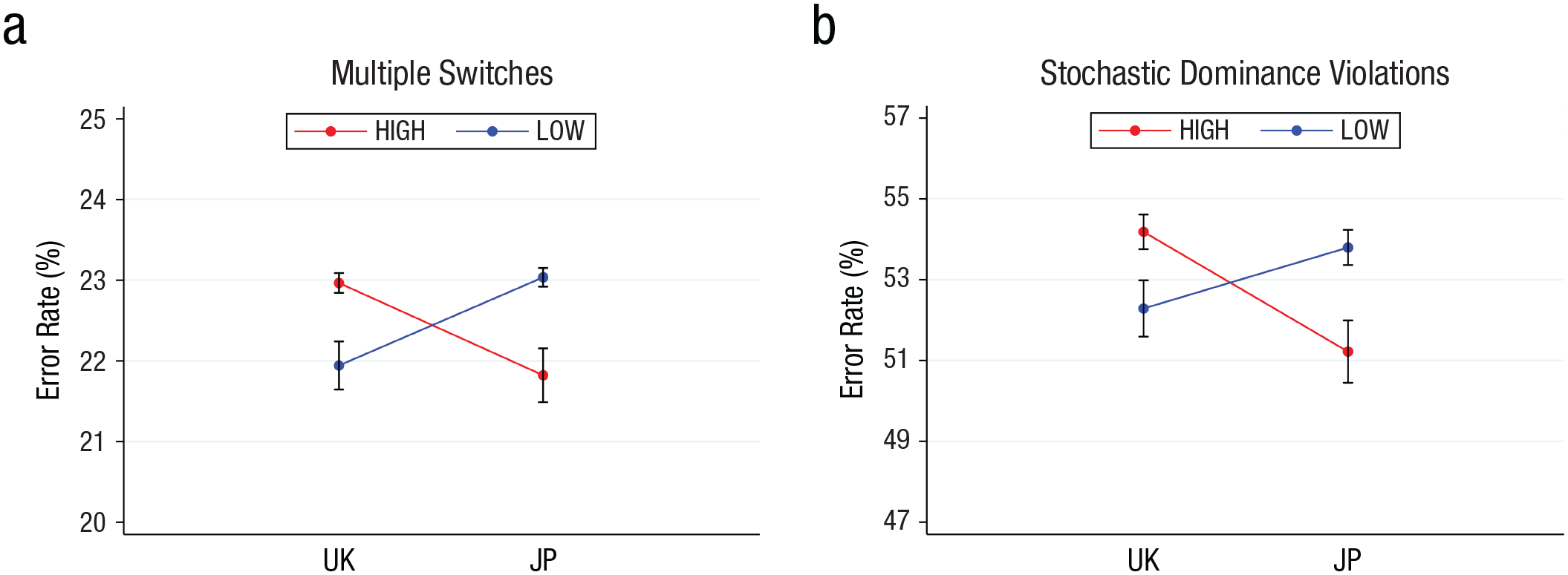
Error rates by country and condition. Error rates between conditions (high vs. low) and countries (UK vs. JP) were defined as the percentage of (a) multiple switches or (b) stochastic dominance violations. According to both definitions, error rates were larger for the nonadapted range of outcomes, UK-high and JP-low, compared with the adapted range, UK-low and JP-high. The asymmetry in error rates between countries can be explained only as range adaptation. UK = United Kingdom; JP = Japan.

We directly tested for the asymmetry between countries with a difference-in-difference test that allowed us to reproduce the results of the single tests. In particular, a panel regression with errors as the dependent variable, dummies for the country (United Kingdom vs. Japan) and condition (high vs. low), and their respective interactions revealed that the asymmetry was statistically significant, M = −2.234, SE = 0.241, p < .001, 95% CI = [−2.706, −1.762] (Table 1, Model 1). The results remained qualitatively unchanged when we controlled for demographic factors such as age, income, gender, and risk attitudes (Table 1, Model 2).

The error rates of the two countries when comparing their respective adapted and nonadapted range were virtually indistinguishable (UK-low vs. JP-high WRS: N = 1,147, z = 0.37, p = .712; UK-high vs. JP-low WRS: N = 1,162, z = −0.64, p = .525), indicating that the groups were otherwise comparable. Participants were very similar with regard to other characteristics. We found no difference in declared risk tolerance between conditions within each country—UK Wilcoxon signed-rank test (WSR): N = 1,157, z = 0.82, p = .412; Japan WSR: N = 1,152, z = 1.19, p = .236. We did observe a significant difference in declared risk attitudes (Falk et al., 2018) between countries, with Japanese participants reporting less risk aversion than participants from the United Kingdom (WSR: N = 2,309, z = −14.53, p < .001), which could, however, not explain our results. Although it was not a requisite for our hypotheses that the countries be very similar, it strengthens the conclusion that the main difference between the asymmetry of error rates was due to the different numerical ranges to which people in the different countries were adapted.

When looking at error rates as the percentage of time participants violated stochastic dominance between the paired lists, as shown in Figure 2b, we observed qualitatively identical results (i.e., an error rate of 54.18% for UK-high compared with 52.29% for UK-low). The difference was statistically significant—WRS: N = 1,157, z = 2.46, p = .014, 95% CI = [1.075, 2.714], BF = 0.12, d = 0.27. We once again observed the opposite pattern for Japanese participants, with an error rate of 51.22% for JP-high compared with 53.79% for JP-low—WRS: N = 1,152, z = −3.44, p < .001, 95% CI = [−3.450, −1.700], BF = 6.36, d = 0.34. We again found that the baseline error rates for adapted and nonadapted ranges were comparable between the two countries (UK-low vs. JP-high WRS: N = 1,147, z = −1.96, p = .050; UK-high vs. JP-low WRS: N = 1,162, z = 1.16, p = .245). A difference-in-difference test confirmed that the asymmetry was significant, M = −4.468, SE = 0.611, p < .001, 95% CI = [−5.667, −3.270] (Table 1, Model 3). The results were again robust after controlling for demographic factors such as age, income, gender, and risk attitudes (Table 1, Model 4).

The number of stochastic dominance violations may seem high, falling in the range of 51% to 54%. Typical figures reported in the literature tend to be significantly smaller at about 15% (Alós-Ferrer & Garagnani, 2022; Khaw et al., 2021). This might suggest that participants were behaving randomly. It is, however, important to keep in mind that we explicitly designed our tasks to detect such violations. In the context of our study, stochastic dominance violations were indirect in that they were calculated from the comparisons between A versus C and B versus C, where B stochastically dominated A. Because the payoff difference between A and B was small, the high error rates were not too different from inconsistencies between “repetitions” of identical choice tasks. Following this interpretation, the obtained results are similar to those reported in the literature (e.g., Alós-Ferrer & Garagnani, 2021). Another piece of evidence that tells us that people did not behave randomly is that subjects reacted strongly to the expected value difference of the choice options: In the UK-low group, participants chose the option with the highest expected value in 72.02% of cases, and in the UK-high group, participants chose this option in 72.90% of cases; in the JP-low group, participants chose the option with the highest expected value in 72.34% of cases, and in the JP-high group, participants chose this option in 70.93% of cases. All four percentages were different from random choice according to a nonparametric (WRS) test (p < .001), indicating behavior that was clearly distinct from pure noise.

Finally, we investigated potential differences in risk taking resulting from numerical adaptation. This comes with the caveat that our experiment was not designed to be diagnostic of differences in risk taking per se so that we could have low power to detect potential differences in risk taking (if any existed). In particular, we investigated potential differences between the adapted and the nonadapted range in the percentage of choices for the safer option, the lottery that involved definitely earning some money compared with taking a risk and potentially earning nothing. We observed no differences in risk attitudes between treatments within each country (UK-high 51.20% vs. UK-low 50.98% WSR: N = 1,157, z = 0.18, p = .859; JP-high 50.52% vs. JP-low 50.65% WSR: N = 1,152, z = −0.09, p = .927).

One interesting question concerns whether we would observe any adaptation to the numerical magnitudes used in the experiment over the 160 tasks used. Our experimental design used four different blocks of 40 tasks each, which gave us equal power to test for the occurrence of errors during different phases of the experiment. We could do this because both definitions of errors were based on an ordered lists of 10 trials that were presented in pseudorandomized order to participants such that within each block the order in which participants saw a trial was random but blocks were kept separate. Tasks within each of these blocks were randomized.

Figure 3 shows the results. In both the United Kingdom and Japan, inconsistencies within lists declined between Blocks 1 and 2—UK-high WSR: 22.847% vs. 18.759% (N = 576, z = 16.02, p < .001); UK-low WSR: 21.915% vs. 18.386% (N = 581, z = 14.93, p < .001); JP-high WSR: 21.418% vs. 17.999% (N = 566, z = 14.34, p < .001); JP-low WSR: 22.367% vs. 18.959% (N = 586, z = 14.01, p < .001)—and between Blocks 3 and 4—UK-high WSR: 27.625% vs. 22.626% (N = 576, z = 16.99, p < .001); UK-low WSR: 26.213% vs. 21.256% (N = 581, z = 17.15, p < .001); JP-high WSR: 26.303% vs. 21.568% (N = 566, z = 17.05, p < .001); JP-low WSR: 27.747% vs. 23.063% (N = 586, z = 16.994, p < .001)—but jumped up markedly between Blocks 2 and 3, as shown in Figures 3a and 3b (UK-high WSR: N = 576, z = 19.15, p < .001; UK-low WSR: N = 581, z = 18.49, p < .001; JP-high WSR: N = 566, z = 18.35, p < .001; JP-low WSR: N = 586, z = 18.82, p < .001). We conclude from this that there was no clear trend overall. We also could not detect a clear trend in differences across treatments within either country—our main interest here. Although multiple switching seems to have decreased between Blocks 1 and 2 in the United Kingdom (WRS: N = 1,157, z = 2.23, p = .026), there was no equivalent tendency in Japan (WRS: N = 1,157, z = −0.83, p = .409), and errors seem to have increased again in subsequent rounds. We conclude from this that there was no systematic adaptation visible in within-lists inconsistencies.

Fig. 3.

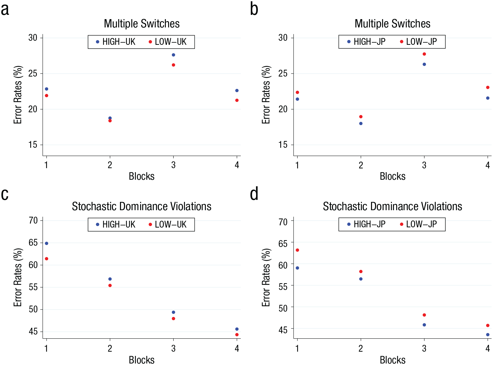
Error rates across blocks of 40 tasks. Error rates between conditions (high vs. low) across blocks of the experiment and countries (UK vs. JP) were defined as (a, b) the percentage of multiple switches or (c, d) the percentage of stochastic dominance violations. UK = United Kingdom; JP = Japan.

As shown in Figures 4c and 4d, stochastic dominance violations clearly decreased over time in both the United Kingdom and Japan and across treatments, that is, for all comparisons such that Block j > i led to v_j < v_i error rates with p < .010. The evolution of the difference between treatments, however, was again less clear. In particular, although we did not see a decline in the difference between treatments from the first to the second block in both countries (UK WSR: N = 1,157, z = 2.33, p = .020; JP WRS: N = 1,152, z = −2.27, p = .023), the difference appears to have remained stable thereafter (UK Block 2 vs. Block 3 WSR: N = 1,157, z = −0.25, p = .807; JP Block 2 vs. Block 3 WRS: N = 1,152, z = 0.74, p = .458; UK Block 3 vs. Block 4 WSR: N = 1,157, z = 0.07, p = .946; JP Block 3 vs. Block 4 WRS: N = 1,152, z = 0.16, p = .870). To the extent that there may have been any adaptation, this adaptation thus seems to have been quick initially but to slow down over time and to be highly incomplete. Longer test runs may thus be needed to conclusively show adaptation at work.

Study 2: Replication Study in Austria and Hungary

Method

Although we took good care to identify our main effects of interest using a difference-in-difference design, systematic differences between two countries as diverse as the United Kingdom and Japan could still result in confounds. We thus replicated the results presented in the first study in two additional countries. Specifically, we replicated our study in Austria and Hungary. These two countries share a border and are closely linked culturally and historically, but once again their currency units are vastly different. Austria has the euro and Hungary the forint, with 1 euro corresponding to about 400 forints (1 forint is 0.0025 euros). This gives us a similar variation in natural currency units as the one between the United Kingdom and Japan exploited in our main study.

The design of the replication study was the same as the main study, with only some minor differences to fit the study situation. Although we used the exact same stimuli, we adapted the multiplier to fit the difference in currency units. Specifically, the outcomes of the lotteries in the “high” conditions (AU-high and HU-high) were obtained by multiplying the outcomes in the “low” conditions (AU-low and HU-low) by 400. Because all effect sizes in the first study were above 0.3, we required only 290 participants (145 in each condition and country) to achieve a power of .8 for a between-subjects test. We conservatively aimed to recruit 300 participants per country (150 for the low condition and 150 for the high condition) and conducted the study on Prolific—an online platform for survey and experimental studies. All instructions were in English because participants are used to this language while doing experiments on Prolific.

We ended up obtaining data from 607 participants (AU-high N = 151, AU-low N = 151, HU-high N = 154, HU-low N = 151). Participants received a fixed payment of 3 pounds for participation in the study, which took about 18 min. In addition, for each participant one choice among the 160 was randomly selected to be played for real money.

Results

Figure 4 shows the main results. Austrian participants displayed larger error rates in the high condition than in the low condition, which fully replicated the results obtained for the United Kingdom in the primary study. The exact opposite could be observed for participants from Hungary, in which those in the high group committed fewer errors than those in the low group, fully replicating the results for Japan. Our key predictions thus replicated—error rates were highest outside of the habitual range regardless of whether that range entailed large nominal payoffs or small nominal payoffs. These results were once again robust regardless of which definition of errors we used. When looking at multiple switches within each list, as shown in Figure 4a, we observed an error rate of 23.28% for the AU-high group compared with 21.35% for the AU-low group, which was an increase of 9.04% in error rates from the adapted to the nonadapted range. The difference was statistically significant—WRS: N = 302, z = 8.88, p < .001, 95% CI = [1.552, 2.306], BF = 25.54, d = 1.00. This difference in error rates translated into a statistically significant drop in subjects’ earnings from 16.97 to 16.22 pounds (4.42%, 0.75 pounds)—WRS: N = 302, z = 2.23, p = .026, 95% CI = [0.092, 1.418], BF = 3.17, d = 0.26. We observed an error rate of 21.02% for the HU-high group compared with 23.46% for the HU-low group, which was an increase of about 11.61% in error rates from the adapted to the nonadapted range (Fig. 4a). The difference was again statistically significant— WRS: N = 305, z = −10.67, p < .001, 95% CI = [−2.811, −2.063], BF = 44.46, d = 1.19. This difference in error rates translated again into a statistically significant drop in subjects’ earnings from 19.74 to 16.77 pounds (15.05%, 2.96 pounds)—WRS: N = 305, z = 12.93, p < .001, 95% CI = [2.573, 3.351], BF = 78.09, d = 1.30.

Fig. 4.

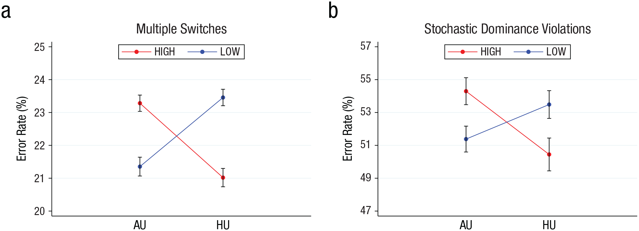
Error rates by country and condition. Error rates between conditions (high vs. low) and countries (AU vs. HU) were defined as the percentage of (a) multiple switches or (b) stochastic dominance violations. According to both definitions, error rates were larger for the nonadapted range of outcomes, AU-high and HU-low, compared with the adapted range, HU-low and AU-high. The asymmetry in error rates between countries can be explained only as range adaptation. AU = Austria; HU = Hungary.

We directly tested for the asymmetry between countries with a difference-in-difference test, which allowed us to reproduce the results of the single tests. In particular, a panel regression with errors as the dependent variable, dummies for the country (Austria vs. Hungary) and condition (high vs. low), and their respective interactions revealed that the asymmetry was statistically significant, M = −4.367, SE = 0.267, p < .001, 95% CI = [−4.891, −3.844] (Table 2, Model 1). The results remained qualitatively unchanged when we controlled for demographic factors such as age, income, gender, and risk attitudes (Table 2, Model 2).

The error rates of the two countries when comparing their respective adapted and nonadapted range were virtually indistinguishable (AU-low vs. HU-high WRS: N = 305, z = −1.42, p = .154; AU-high vs. HU-low WRS: N = 302, z = −1.00, p = .316), indicating that the groups were otherwise comparable. Participants were very similar with regard to other characteristics. We found no difference in declared risk tolerance between conditions within each country (AU WSR: N = 302, z = 0.14, p = .891; HU WSR: N = 305, z = −0.77, p = .440). We did not observe a significant difference in declared risk attitudes (Falk et al., 2018) between countries (WSR: N = 607, z = 1.59, p = .112).

When looking at error rates as the percentage of time participants violated stochastic dominance between the paired lists, as shown in Figure 4b, we observed qualitatively identical results (i.e., an error rate of 54.30% for the AU-high group compared with 51.38% for the AU-low group). The difference was statistically significant—WRS: N = 302, z = 4.83, p < .001, 95% CI = [1.782, 4.046], BF = 2.27, d = 0.56. We once again observed the opposite pattern for Hungarian participants, with an error rate of 50.45% for the HU-high group compared with 53.49% for the HU-low group—WRS: N = 305, z = −4.30, p < .001, 95% CI = [−4.342, −1.735], BF = 0.40, d = 0.51. We again found that the baseline error rates for adapted and nonadapted ranges were comparable between the two countries (AU-low vs. HU-high WRS: N = 305, z = −1.41, p = .158; AU-high vs. HU-low WRS: N = 302, z = 1.37, p = .170). A difference-in-difference test confirmed that the asymmetry was significant, M = −5.953, SE = 0.878, p < .001, 95% CI = [−7.674, −4.231] (Table 2, Model 3). The results were again robust after controlling for demographic factors such as age, income, gender, and risk attitudes (Table 2, Model 4).

Last, we again investigated potential differences in risk taking resulting from numerical adaptation. We observed statistically significant differences in risk attitudes between treatments within each country in the direction of more risk tolerance for the nonadapted range—AU-high 51.88% vs. AU-low 61.74% WSR: N = 302, z = −14.61, p < .001, 95% CI = [−10.56, −9.18], BF = 176.12, d = 1.70; HU-high 61.44% vs. HU-low 51.35% WSR: N = 305, z = 14.93, p < .001, 95% CI = [9.45, 10.74], BF = 196.14, d = 1.74. We report the results of the adaptation analysis for the second study in the Supplemental Material. We reproduced qualitatively the same results obtained in the previous study. Overall, we fully replicated the results of the first study with two different countries using a different range of adapted numbers.

Discussion

Our ability to discriminate between stimuli depends on how familiar we are with them, a phenomenon that we refer to as “efficient numerical range adaptation.” This principle, which derives from an efficient use of our constrained neural resources, is a robust finding in psychophysics, for example, when examining perceptual discrimination of colors or lengths. Recently, it has been applied to decision-making in economics (e.g. Frydman & Jin, 2022; Khaw et al., 2021; Polania et al., 2019; Prat-Carrabin & Woodford, 2022; Vieider, 2023). However, most empirical tests have been limited to relatively small samples of standard subject pools in laboratory settings, such as the test of decision-by-sampling predictions about loss aversion by Walasek and Stewart (2014) and the test of efficient coding adaptation presented by Frydman and Jin (2022).

The question of how important range adaptation is for real-world situations and whether it can be found as a by-product of naturally occurring variation in economically relevant quantities remains largely open. Here we quantified the importance and economic magnitude of range adaptation in the field. In particular, we exploited natural variation in numerical currency units across countries as a proxy for the numerical ranges people are adapted to for economically relevant choices. This allowed us to show that people make substantially more mistakes in their nonadapted range. At 5% or more, the differences in error rates when making choices in the habitual numerical range versus a nonadapted range were of medium size (they were large in the replication in Austria and Hungary) and clearly significant from an economic as well as a statistical point of view. At between 5% and 13% of potential earnings foregone because of these additional mistakes, the economic effects of these tests were also highly significant. That is, people’s quality of economically relevant choices strictly depends on the range they are adapted to, which we showed to depend on their country of residence.

It seems quite natural that currency units would play a major role for the numerical range to which people adapt. Small currency transactions are ubiquitous and will be encountered dozens of times a day (e.g., during grocery shopping, when checking one’s bills or account balance). Stewart et al. (2006) indeed implicitly included narrow framing into their model of decision by sampling, whereby credits count for the valuation of gains and debits toward the valuation of losses (whereas time delays count toward discounting and probability statements toward likelihood assessment). Other numerical units, such as those used for weights or distances, are arguably more similar between countries. Although there may be some degree of difference between countries because of the use of different measurement units—for example, because of the use of pounds (or stones) versus kilograms, yards (or feet) versus meters, miles versus kilometers, or inches versus centimeters—these differences fall far short of the two orders of magnitude we observed for currency units. They also often go in opposite directions (e.g., feet vs. meters, inches vs. centimeters), meaning that they were unlikely to confound our treatment (and they did not apply in the case of Austria vs. Hungary). We thus argue that such small numbers being present in both countries—and being relatively similar on average—might make it more difficult to find the type of results we documented, making it all the more remarkable that they did indeed emerge in the data.

We found the asymmetry in mistakes using two definitions of errors. We looked at the number of inconsistencies in an ordered list of choices in which people’s preferences normatively implied only one switch. We documented that people were clearly less consistent in their nonadapted range. The literature has interpreted such “multiple switches” as misunderstanding of the task (Holt & Laury, 2005) or lower cognitive abilities (Yu et al., 2021). We can exclude this as an explanation for our results because we randomly assigned participants drawn from the same representative subject pool to adapted versus nonadapted ranges. An alternative explanation for multiple switches proposed by the literature is preference imprecision (e.g., Chew et al., (2022). This is in line with our findings if imprecision in the perception of the numbers directly translates into imprecision in the implied preferences (Khaw et al., 2021). Note once more that avoiding both types of errors in our setting did not require calculations of the expected (subjective) values of the options. The only element needed for avoiding errors was numerical comparison, which entailed that “more is better” in all our experimental treatments.

Our experiments were directly geared at investigating whether adaptation to a certain numerical range would impact error rates. Such effects are not foreseen by standard models of decision-making, such as expected utility theory or prospect theory, which have traditionally taken little interest in errors. They are, on the other hand, a direct implication of a wide class of adaptive models that postulate that the mind leverages adaptive mechanisms as a way of dealing with cognitive limitations. Our test was explicitly devised to examine the broad implication of this entire class of models in the natural context of adaptation to the numerical units of national currency units.

This is not to say, however, that these models are identical. Even when it comes to errors, adaptive models may differ with respect to where the error occurs exactly. For instance, in the decision-by-sampling model, the error occurs at the level of utility attribution because of the comparison to a small number of samples drawn from memory (Stewart, 2009; Stewart et al., 2006). Similar errors occur at the level of utility assignment in the models by Robson (2001) and Netzer (2009) because people are unable to assign arbitrarily small utility differences and thus allocate their discrimination thresholds where they matter the most. In the noisy cognition model of Khaw et al. (2021), on the other hand, errors will occur at the level of numerical perception itself.⁶

These adaptive models furthermore differ with respect to the predictions they make in terms of the risk-taking patterns one ought to observe in different situations. Our tasks were not devised to test such differences—which are often intricate and very specific—or, for that matter, to test differences in risk taking at all (see Supplemental Material for a discussion of the predictions of decision-by-sampling as an example). Thus, although our data show general support for adaptive models of choice, they are ill suited to discriminate between the different models in this class and their specific predictions.

Our results highlight the direct and significant economic importance of numerical adaptation for real-world settings. Our findings are thus of direct relevance to decisions that are typically made in nonadapted ranges from investments in foreign stock markets into cryptocurrencies and gambling in online casinos to cross-boarder shopping. In this sense, these results also provide a microfoundation for the money illusion phenomenon (Shafir et al., 1997) and its economic consequences (Fehr & Tyran, 2001, 2007). Our results suggest that a possible reason why research on money illusion has found mixed empirical effects (e.g., Desmet, 2002; Gamble et al., 2002; Raghubir & Srivastava, 2002) is that its determinants were unclear. People are not expected to make the worst choices just because the monetary amounts are labeled differently, as usually assumed in this literature. Our results specifically predict money illusion to be stronger when people make choices using nominal currency units falling into nonadapted ranges. Finally, our results may also provide an explanation for why error rates have been found to increase in stakes even when such stakes are real (Enke et al., 2023)—a finding that may otherwise appear paradoxical from an economic point of view. The wider implications of our findings are that cognitive resource limitations clearly impact economically relevant decisions. Integrating such limitations into economic models should thus be a priority for future research.

Supplemental Material

sj-pdf-1-pss-10.1177_09567976251339195 – Supplemental material for Economic Consequences of Numerical Adaptation

Supplemental material, sj-pdf-1-pss-10.1177_09567976251339195 for Economic Consequences of Numerical Adaptation by Michele Garagnani and Ferdinand M. Vieider in Psychological Science

Footnotes

Transparency

Action Editor: Ulrike Hahn

Editor: Simine Vazire

Author Contributions

Michele Garagnani: Conceptualization; Data curation; Formal analysis; Investigation; Methodology; Project administration; Resources; Software; Supervision; Validation; Visualization; Writing – original draft; Writing – review & editing.

Ferdinand M. Vieider: Conceptualization; Data curation; Formal analysis; Funding acquisition; Investigation; Methodology; Project administration; Resources; Software; Supervision; Validation; Visualization; Writing – original draft; Writing – review & editing.

ORCID iD

Michele Garagnani

Supplemental Material

Additional supporting information can be found at

Notes

References

Alós-Ferrer

Fehr

Netzer

(2021). Time will tell: Recovering preferences when choices are noisy. Journal of Political Economy, 129(6), 1828–1877.

Alós-Ferrer

Garagnani

(2021). Choice consistency and strength of preference. Economics Letters, 198, Article 109672. https://doi.org/10.1016/j.econlet.2020.109672

Alós-Ferrer

Garagnani

(2022). The gradual nature of economic errors. Journal of Economic Behavior & Organization, 200, 55–66.

Bhui

Lai

Gershman

S. J.

(2021). Resource-rational decision making. Current Opinion in Behavioral Sciences, 41, 15–21.

Chew

S. H.

Miao

Shen

Zhong

(2022). Multiple-switching behavior in choice-list elicitation of risk preference. Journal of Economic Theory, 204, Article 105510. https://doi.org/10.1016/j.jet.2022.105510

Cohn

Engelmann

Fehr

Maréchal

M. A.

(2015). Evidence for countercyclical risk aversion: An experiment with financial professionals. American Economic Review, 105(2), 860–885.

Desmet

(2002). A study of the potential effects of the conversion to euro. Journal of Product & Brand Management, 11, 134–146.

Di Falco

Vieider

F. M

. (2022). Environmental adaptation of risk preferences. Economic Journal, 132(648), 2737–2766.

Dohmen

Falk

Huffman

Sunde

Schupp

Wagner

G. G.

(2011). Individual risk attitudes: Measurement, determinants, and behavioral consequences. Journal of the European Economic Association, 9(3), 522–550.

10.

Enke

Graeber

Oprea

(2023). Complexity and time (CESifo Working Paper No. 10327). SSRN. https://doi.org/10.2139/ssrn.4402494

11.

Falk

Becker

Dohmen

Enke

Huffman

Sunde

(2018). Global evidence on economic preferences. Quarterly Journal of Economics, 133(4), 1645–1692.

12.

Fehr

Tyran

J.-R.

(2001). Does money illusion matter? American Economic Review, 91(5), 1239–1262.

13.

Fehr

Tyran

J.-R.

(2007). Money illusion and coordination failure. Games and Economic Behavior, 58(2), 246–268.

14.

Frydman

Jin

L. J.

(2022). Efficient coding and risky choice. The Quarterly Journal of Economics, 137(1), 161–213.

15.

Gamble

Gärling

Charlton

Ranyard

(2002). Euro illusion: Psychological insights into price evaluations with a unitary currency. European Psychologist, 7(4), 302.

16.

Garagnani

(2023). The predictive power of risk elicitation tasks. Journal of Risk and Uncertainty, 67, 165–192.

17.

Garcia

M. B.

de Hollander

Grueschow

Polania

Woodford

Ruff

C. C.

(2023). Individual risk attitudes arise from noise in neurocognitive magnitude representations. Nature Human Behaviour, 7, 1551–1567.

18.

Heng

J. A.

Woodford

Polania

(2020). Efficient sampling and noisy decisions. Elife, 9, Article e54962. https://doi.org/10.7554/eLife.54962

19.

Holt

C. A.

Laury

S. K.

(2002). Risk aversion and incentive effects. American Economic Review, 92(5), 1644–1655.

20.

Holt

C. A.

Laury

S. K.

(2005). Risk aversion and incentive effects: New data without order effects. American Economic Review, 95(3), 902–904.

21.

Kahneman

Tversky

(1979). Prospect theory: An analysis of decision under risk. Econometrica, 47(2), 263–291.

22.

Khaw

M. W.

Glimcher

P. W.

Louie

(2017). Normalized value coding explains dynamic adaptation in the human valuation process. Proceedings of the National Academy of Sciences, USA, 114(48), 12696–12701.

23.

Khaw

M. W.

Woodford

(2021). Cognitive imprecision and small-stakes risk aversion. The Review of Economic Studies, 88(4), 1979–2013.

24.

Laughlin

(1981). A simple coding procedure enhances a neuron’s information capacity. Zeitschrift für Naturforschung C., 36(9–10), 910–912.

25.

Laughlin

S. B.

de Ruyter van Steveninck

R. R.

Anderson

J. C.

(1998). The metabolic cost of neural information. Nature Neuroscience, 1(1), 36–41.

26.

Lieder

Griffiths

T. L.

(2020). Resource-rational analysis: Understanding human cognition as the optimal use of limited computational resources. Behavioral and Brain Sciences, 43, Article e1. https://doi.org/10.1017/S0140525X1900061X

27.

Lipkus

I. M.

Samsa

Rimer

B. K.

(2001). General performance on a numeracy scale among highly educated samples. Medical Decision Making, 21(1), 37–44.

28.

Louie

Glimcher

P. W.

Webb

(2015). Adaptive neural coding: From biological to behavioral decision-making. Current Opinion in Behavioral Sciences, 5, 91–99.

29.

Netzer

(2009). Evolution of time preferences and attitudes toward risk. American Economic Review, 99(3), 937–955.

30.

Oprea

(2024). Decisions under risk are decisions under complexity. American Economic Review, 114(12), 3789–3811.

31.

Padoa-Schioppa

(2009). Range-adapting representation of economic value in the orbitofrontal cortex. Journal of Neuroscience, 29(44), 14004–14014.

32.

Padoa-Schioppa

Conen

K. E.

(2017). Orbitofrontal cortex: A neural circuit for economic decisions. Neuron, 96(4), 736–754.

33.

Piazza

Izard

Pinel

Le Bihan

Dehaene

(2004). Tuning curves for approximate numerosity in the human intraparietal sulcus. Neuron, 44(3), 547–555.

34.

Polania

Woodford

Ruff

C. C.

(2019). Efficient coding of subjective value. Nature Neuroscience, 22(1), 134–142.

35.

Prat-Carrabin

Woodford

(2022). Efficient coding of numbers explains decision bias and noise. Nature Human Behaviour, 6, 1142–1152.

36.

Raghubir

Srivastava

(2002). Effect of face value on product valuation in foreign currencies. Journal of Consumer Research, 29(3), 335–347.

37.

Robson

A. J.

(2001). The biological basis of economic behavior. Journal of Economic Literature, 39(1), 11–33.

38.

Rustichini

Conen

K. E.

Cai

Padoa-Schioppa

(2017). Optimal coding and neuronal adaptation in economic decisions. Nature Communications, 8, Article 1208. https://doi.org/10.1038/s41467-017-01373-y

39.

Shafir

Diamond

Tversky

(1997). Money illusion. Quarterly Journal of Economics, 112(2), 341–374.

40.

Stewart

(2009). Eps prize lecture: Decision by sampling: The role of the decision environment in risky choice. Quarterly Journal of Experimental Psychology, 62(6), 1041–1062.

41.

Stewart

Chater

Brown

G. D.

(2006). Decision by sampling. Cognitive Psychology, 53(1), 1–26.

42.

Stewart

Reimers

Harris

A. J.

(2014). On the origin of utility, weighting, and discounting functions: How they get their shapes and how to change their shapes. Management Science, 61(3), 687–705.

43.

Vieider

F. M.

(2023). Cognitive foundations of delay-discounting. IDEAS.

44.

Vieider

F. M.

(2024). Decisions under uncertainty as Bayesian inference on choice options. Management Science, 70(12), 9014–9030.

45.

von Neumann

Morgenstern

. (1944). Theory of games and economic behavior. Princeton University Press.

46.

Walasek

Stewart

(2014). How to make loss aversion disappear and reverse: Tests of the decision by sampling origin of loss aversion. Journal of Experimental Psychology: General, 144(1), 7–11.

47.

Webb

Glimcher

P. W.

Louie

(2020). Divisive normalization does influence decisions with multiple alternatives. Nature Human Behaviour, 4(11), 1118–1120.

48.

C. W.

Zhang

Y. J.

Zuo

S. X.

(2021). Multiple switching and data quality in the multiple price list. Review of Economics and Statistics, 103(1), 136–150.

49.

Zhang

Ren

Maloney

L. T.

(2020). The bounded rationality of probability distortion. Proceedings of the National Academy of Sciences, USA, 117(36), 22024–22034.

Supplementary Material

Please find the following supplemental material available below.

For Open Access articles published under a Creative Commons License, all supplemental material carries the same license as the article it is associated with.

For non-Open Access articles published, all supplemental material carries a non-exclusive license, and permission requests for re-use of supplemental material or any part of supplemental material shall be sent directly to the copyright owner as specified in the copyright notice associated with the article.

0.00 MB

0.17 MB