Sage Journals: Discover world-class research

Abstract

Boundary extension is a classic memory illusion in which observers remember more of a scene than was presented. According to predictive-processing accounts, boundary extension reflects the integration of visual input and expectations of what is beyond a scene’s boundaries. According to normalization accounts, boundary extension rather reflects one end of a normalization process toward a scene’s typically experienced viewing distance, such that close-up views give boundary extension but distant views give boundary contraction. Here, across four experiments (N = 125 adults), we found that boundary extension strongly depends on depth of field, as determined by the aperture settings on a camera. Photographs with naturalistic depth of field led to larger boundary extension than photographs with unnaturalistic depth of field, even when distant views were shown. We propose that boundary extension reflects a predictive mechanism with adaptive value that is strongest for naturalistic views of scenes. The current findings indicate that depth of field is an important variable to consider in the study of scene perception and memory.

Keywords

boundary extension natural vision predictive processing scene memory visual perception open data open materials

Boundary extension is a classic memory illusion in which observers remember more of a scene than was actually presented (Intraub & Richardson, 1989). For example, when participants draw a previously observed scene, they typically include information not present in the photograph, expanding the scene beyond its boundaries (Intraub & Richardson, 1989). Similarly, when rating the viewpoint of a second probe photograph relative to a remembered target photograph, participants rate the exact same view as closer than the original image, indicating that they remembered more of the scene than was presented (Bainbridge & Baker, 2020; Bertamini et al., 2005; Dickinson & Intraub, 2008; Intraub & Dickinson, 2008).

Why does this illusion occur? One possibility is that it reflects a predictive mechanism in which scene percepts do not correspond solely to the visual input but are rather constructed through integration of visual input and expectations of what is beyond a scene’s boundaries (Intraub, 2010; Maguire & Mullally, 2013). The discrete views sampled by the human eye may thus be supplemented with anticipatory representations of the scene, providing a continuous visual experience.

Alternatively, boundary extension may reflect one end of a generic normalization process in memory (Bartlett, 1932), where the perceived scene viewpoint regresses toward a prototypical viewing distance: A view that is close up compared with the observer’s average viewing distance of that scene will be remembered as farther away (yielding boundary extension), whereas faraway views will be remembered as being closer, generating the opposite error, boundary contraction. On this account, boundary extension and boundary contraction are in principle equally common, depending only on whether the presented photographs are taken from a relatively close or far distance.

Previous work has shown that boundary extension occurs more frequently than boundary contraction (Hubbard et al., 2010; Intraub, 2020). Furthermore, boundary extension occurs for scenes but not for single, isolated objects (Gottesman & Intraub, 2002; Intraub et al., 1998), unlike normalization, which also occurs for isolated objects (Brady et al., 2011; Intraub et al., 1998; Konkle & Oliva, 2007). However, although these results appear to show that boundary extension cannot be entirely accounted for by normalization, this conclusion relies on the strong assumption that the scene photographs used in previous work were representative of our daily-life visual experience, particularly with respect to viewing distance. If the photographs used in boundary extension studies were not representative—for example, if they primarily showed views that were closer than usually experienced—boundary extension may be entirely explained by a normalization account.

Indeed, using a large and diverse stimulus set (1,000 photographs), a recent study showed that boundary extension was equally as common as boundary contraction (Bainbridge & Baker, 2020). Moreover, the direction of these memory errors was correlated with ratings of subjective image distance: In line with the normalization account, subjectively close scenes tended to extend, and subjectively far scenes tended to contract. These results suggest that boundary extension may be one side of a regression toward the typical scene-viewing distance.

The above discussion highlights that approximating daily-life visual experience is critical for both accounts: for the predictive-processing account because it proposes that boundary extension reflects expectations based on real-world experience and for the normalization account because normalization is relative to our prior experience. If boundary extension reflects expectations, it should be observed more prominently (and be more common than boundary contraction) when views are representative of our visual experience. Importantly, this is not automatically achieved through the use of large and diverse image sets. Even if these are representative of pictorial views of scenes (i.e., of how scene photographs are taken), they are not necessarily representative of how an observer perceives their surroundings during day-to-day visual experience.

A striking example is that a camera can produce pictures with a deeper depth of field than the eye can (Artal, 2014; Middleton, 1957). The depth of field represents the distance range over which an object may be moved without causing a sharpness reduction. On a camera, depth of field can be controlled by the lens aperture, typically specified by an f-number (focal length divided by aperture diameter). The eye’s depth of field similarly depends on the aperture of the pupil. The larger the aperture, the shallower the depth of field, resulting in a smaller distance range within which objects are in focus. The aperture range of most cameras is much larger than that of the eye, which ranges between f/2.1 and f/8. Specifically, photographs often have very deep depth of field (e.g., f/22): Everything in the picture is sharp, leading to views of scenes that are highly unnatural.

Statement of Relevance

In daily life, we experience a rich and continuous visual world in spite of the capacity limits of the visual system. We may compensate for such limits with our memory, by filling in the visual input with anticipatory representations of upcoming views. The boundary extension illusion provides a tool to investigate this phenomenon. For example, not all images equally lead to boundary extension. In this set of experiments, we found that memory extrapolation beyond scene boundaries was strongest for images resembling human visual experience, showing depth of field in the range of human vision. On the basis of these findings, we propose that predicting upcoming views is conditional to a scene being naturalistic. More generally, the strong reliance of a cognitive effect, such as boundary extension, on naturalistic image properties indicates that it is imperative to use image sets that are ecologically representative when studying the cognitive, computational, and neural mechanisms of scene processing.

Here, we found that boundary extension strongly depends on depth of field, as determined by the aperture settings on a camera. Reanalyzing the 1,000-image dataset (Bainbridge & Baker, 2020), we found that boundary extension was much more common than boundary contraction for photographs with depths of field within the range of human vision. Subsequently, in three experiments, we demonstrated the specific influence of depth of field on boundary extension while controlling for factors that may naturally covary with depth of field in scene photographs, including viewing distance, number and type of objects, and image statistics. Again, boundary extension was strongest for the relatively shallow depth of field that characterizes human vision and was observed even for distant views of scenes. Altogether, our results are most in line with views of boundary extension as a predictive mechanism, with boundary extension reliably observed for naturalistic views of scenes to which the brain has adapted.

Open Practices Statement

All data and stimuli for these experiments have been made publicly available via OSF and can be accessed at https://osf.io/7btfq/. The design and analysis plans for the experiments were not preregistered. Video demonstrations of the experimental procedures are available at https://sites.google.com/view/marcogandolfo/online-experiments/boundary-extension-and-depth-of-field?pli=1.

Experiment 1

Our goal in Experiment 1 was to test for a relationship between the perceived depth of field of a photograph and its boundary transformation scores (boundary extension or boundary contraction) in the large image set used by Bainbridge and Baker (2020). To this end, we collected aperture ratings (as judged from depth of field) for each of the 1,000 scenes and related these ratings to the boundary transformation scores made available in the original study. On the basis of the predictive-processing account, we hypothesized that the more an image would be rated as having been shot with a large aperture—resembling natural vision—the more strongly it would elicit boundary extension.

Method

Participants

Twenty-six participants (22 females, age: M = 24.5, SD = 5.84) signed up for the online scene-rating experiment. Participants were recruited through Radboud University’s participant panel (Sona Systems) in return for course credits and through social media. The experiment was advertised as being for people who knew the basics of photography. To further ensure participants’ expertise, prior to the scene ratings, we administered a photography quiz. First, participants were asked to define their photography experience with a multiple-choice question: “How would you define your experience with photography? 1) Only took pictures with my smartphone; 2) Some knowledge, but no hands-on experience with Single-Lens-Reflex (SLR) cameras; 3) Some experience using SLR cameras; 4) (Semi-) Professional photographer.” Second, participants had to complete a quiz with five multiple-choice questions. Four of these questions asked how a photograph would look if shot with a large aperture (i.e., shallow depth of field, lots of light entering the camera) and a small aperture (i.e., deep depth of field, little light entering the camera). Finally, one question asked whether a lens aperture of f/5.6 was larger or smaller than f/22.0, testing their knowledge of f-stop values. On the basis of the above questions, we excluded six participants because they declared they had no experience with single-lens-reflex photography (n = 3) or because they failed three or more questions out of five in the photography quiz (two participants had four errors, and one participant had five errors). Among the 20 included participants, only five had one or two errors (two participants had one error, and three participants had two errors). Quiz data for all the participants are available at https://osf.io/7btfq/. This experiment was approved by the Ethics Committee of Radboud University’s Faculty of Social Sciences (ECSW2017-2306).

Stimuli and apparatus

Stimuli were taken from the study by Bainbridge and Baker (2020) and consisted of 1,000 images from their rapid serial visual presentation (RSVP) experiments. These were downloaded from the OSF link (https://osf.io/28nzt/). Further, for the practice trials, 24 images were downloaded from Shutterdial (https://www.shutterdial.com). This website allows users to search for photos according to their metadata (including aperture) from the flickr application programming interface (API). We selected 12 pictures with large apertures (f ≤ 4) and 12 pictures with small apertures (f ≥ 22.0) so the difference between shallow and deep depth of field would be salient. The experiment was conducted online and coded in JavaScript using the jsPsych toolbox (Version 6.2.0; de Leeuw, 2015). The data were saved on the Pavlovia.org servers (www.pavlovia.org).

Procedure

After the photography quiz, participants were shown the task instructions. Here, the concept of aperture was briefly reexplained. Afterward, each participant was presented with six randomly selected practice images (three with large apertures and three with small apertures). In the practice session, participants simply had to report whether an image was shot with a large or small aperture. They received feedback after each trial. When the practice session was completed, more detailed example images were presented, this time stressing the continuity of the aperture effect over the depth of field of the pictures. This was achieved by showing images of the same photograph shot at different levels of aperture (i.e., large, middle, small). Finally, participants were informed that they would make the upcoming ratings on a sliding scale from 0 (large aperture) to 100 (small aperture). Each rating trial began with a fixation cross with a random duration of 1 s, 1.25 s, or 1.5 s. Following fixation, participants saw an image appear on screen concurrently with the slider positioned in the middle (aperture = 50). To continue to the next trial, participants had to touch the slider on the scale and press the button “continue” placed below the image and the slider. After every 50 ratings, participants were invited to take a break.

Design

Each participant completed one of four versions of the experiment. Each version included 250 images from the study by Bainbridge and Baker (2020), equally divided between those originally taken from the SUN database (Xiao et al., 2016) and the Google Open Images database (Kuznetsova et al., 2020). The images were presented in random order to each participant. In total, we obtained five aperture ratings for each of the 1,000 stimuli of Bainbridge and Baker (2020), matching the number of subjective distance ratings collected by Bainbridge and Baker (2020).

Analysis

All the analyses were conducted using R (Version 4.0.1; R Core Team, 2020). We calculated the mean aperture rating for each of the 1,000 images. We also split these ratings (from 0 to 100) in five bins of 20—extra large (XL): 0–20, large (L): 21–40, medium (M): 41–60, small (S): 61–80; extra small (XS): 81–100. Afterward, we downloaded the raw data from the 1,000-image RSVP experiments (i.e., Experiments 2 and 3 by Bainbridge & Baker, 2020). We rescored the boundary transformation scores to −1 (closer), 0 (same, only for Experiment 3), and 1 (farther) and calculated the mean boundary transformation score per image. With these two measures, we (a) ran the correlation between mean aperture ratings and the boundary transformation scores and (b) computed the average boundary rating across images in each categorical aperture rating bin (see Figs. 1a and 1b).

Fig. 1.

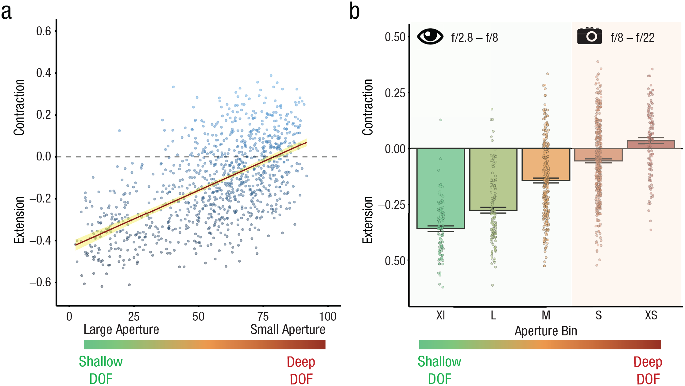
Results from Experiment 1. The scatterplot (a; with best-fitting linear regression line) shows the relation between aperture ratings and boundary transformation scores across the two 1,000-image experiments of Bainbridge and Baker (2020). Images that participants rated as having been shot with large apertures led to strong boundary extension. Images that participants rated as having been shot with small apertures led to less boundary extension or even contraction. The yellow error band around the regression line represents the 95% confidence interval. The bar plot (b) shows average boundary transformation scores across images for each of five aperture bins. Professional photographers judged images in the small (S) and extra small (XS) bins to have been shot with apertures between f/8 and f/22, as computed from comparisons with aperture judgments of pictures with known aperture levels (see the Supplemental Material available online). These apertures are mostly impossible for the human eye. Each data point represents the mean boundary transformation value per image. Error bars represent standard errors of the mean. XL = extra large, L = large, M = medium.

Results

There was a strong and reliable correlation between rated aperture and boundary transformation score (Fig. 1a; ρ = 0.58, p < .001). Images with a shallow depth of field (large aperture) led to the largest extension effects, whereas images with deep depth of field (small aperture) showed less extension or even contraction. To further inspect this relationship, we created five bins, each representing an interval of 20 on the aperture rating scale (XL: 0–20, L: 21–40, M: 41–60, S: 61–80, XS: 81–100). Compellingly, the bar plot in Figure 1b shows that contraction was reliable, on average, only for images rated as having been shot with a small aperture—t test vs. 0 on the values of the XS bin, t(121) = 2.56, p = .01, d = 0.23, M = 0.03, SE = 0.01, 95% confidence interval (CI) = [0.01, 0.06]). These aperture values are reachable by a camera but not by the human eye (Hecht, 1987; Middleton, 1957; see the Supplemental Material available online for information about how we estimated the f-stop value corresponding to each of the five bins shown in Fig. 1).

Bainbridge and Baker (2020) showed that subjective ratings of viewing distance were correlated with boundary transformation scores, in line with findings of other studies (Hafri et al., 2022; Intraub et al., 1992; J. Park et al., 2021). Images rated as having a close view led to larger extension than images rated as having a faraway view. It is possible that the relationship between rated depth of field and boundary scores observed here was entirely absorbed by the relationship between subjective distance and boundary scores. To address this, we partialed out ratings of subjective distance. The correlation between aperture and boundary scores remained highly reliable (ρ = .29, p < .001), even when the shared variance between depth-of-field ratings and subjective distance ratings was regressed out (see the Supplemental Material for the same analyses splitting by image set and partialing out other available image properties from Bainbridge & Baker, 2020).

Experiments 2 and 3

In Experiment 1, we showed that boundary transformation scores and perceived depth of field were related to each other across a large and diverse set of photographs, thus revealing that a previously unexplored image property affects memory for scene boundaries. However, as is the case for viewing distance (Bainbridge & Baker, 2020), the depth of field of an image may covary with numerous other visual and semantic properties. For example, images with deep depth of field are more likely to show an outdoor environment. The correlational approach used in Experiment 1 is thus unable to unambiguously ascribe the effects to depth of field (or, indeed, viewing distance). Therefore, to firmly establish an effect of depth of field on boundary extension, we needed to manipulate depth of field while keeping all other properties equal. To do so, we shot the same 32 pictures of outdoor environments with two different camera apertures (f/5.6 and f/22). This factor was crossed with the camera’s focus distance: either on a nearby or on a faraway object in the scene (Fig. 2). If the size of memory distortions depends on how the depth of field of an image resembles natural viewing conditions, then images with shallow depth of field (f/5.6) should show larger extension than images with deep depth of field (f/22), independently of focus distance.

Fig. 2.

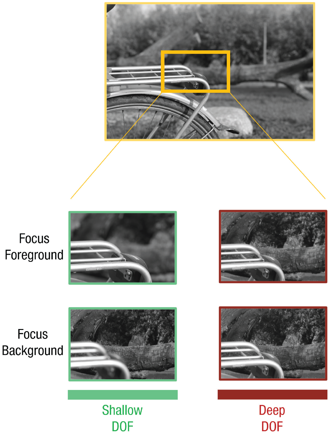
Example of the experimental conditions in Experiments 2 and 3, illustrated by a zoomed-in portion of one of the scene photographs. Each outdoor scene image was shot focusing either on a foreground object or on the background at two levels of aperture: f/5.6 (shallow depth of field [DOF]) and f/22 (deep DOF). The full stimulus set, including the images equated for spatial frequency and histogram used in Experiment 3, is publicly available at https://osf.io/7btfq/.

Method

Participants

The sample size was determined through a power analysis based on the data of a pilot experiment (reported in the Supplemental Material). This analysis revealed that a sample size of 35 participants was required to obtain 80% power to detect a between-conditions difference at least as large as the one observed between the large- and small-aperture conditions in the pilot experiment (reported in the Supplemental Material), on the basis of a paired-samples t contrast. In Experiment 2, 39 participants were recruited (16 females; age: M = 24.66, SD = 4.10) to arrive at a final sample of 35 after exclusions based on missing data or low accuracy (see Analyses). In Experiment 3, 36 participants were recruited (11 females, age: M = 24.36, SD = 4.66). Because of server issues, we obtained only 32 complete data files in Experiment 3 (see Analyses). Participants were recruited via Prolific (www.prolific.co) in return for monetary compensation of £6.31 per hour. Both experiments were approved by the Ethics Committee of Radboud University’s Faculty of Social Sciences (ECSW2017-2306).

Stimuli and apparatus

The stimulus set consisted of six photographs of 32 unique outdoor scenes (192 photographs). Each scene featured one or more objects in the foreground at a distance of approximately 2 m and one or more objects in the background at a distance of at least 5 m. For each scene, six photographs were taken using a digital single-lens reflex (DSLR) camera with a 50-mm fixed focal-length lens placed on a tripod. Photos were shot at three aperture levels—f/5.6 (large), f/11.0 (medium), and f/22 (small)—each one either manually focusing on the foreground objects or on the background objects (see Fig. 2). The medium aperture level was used only in the pilot experiment (see the Supplemental Material). The International Organization for Standardization (ISO) number (light sensitivity of the sensor) was set manually in each scene (but kept constant across aperture and focus variations of that scene), and the shutter speed was automated to achieve similar lighting for the six photographs. We then generated close-view scenes through resizing (without resampling) the original pictures. This was achieved by enlarging the image (i.e., zooming in) using a random percentage value between 17% to 24% (in steps of 0.5%) of the image’s surface area and then cropping the image to its original size. Each scene was enlarged by the same percentage across the scene’s aperture and focus distance levels. All the pictures were then converted to gray scale and resized to 750 × 500 pixels. The images appeared on the screen at this resolution and therefore varied in size depending on the resolution the participants visualized them on their screen. Further, eight different masks were generated by computing the average image of all the photos in the stimulus set and iterating image scrambling in 20 pixel × 20 pixel blocks (randomly scrambling on the x-axis and then on the y-axis, or vice versa). Image processing was performed using the R package imager (Barthelmé & Tschumperlé, 2019).

In Experiment 3, we matched the stimuli for low-level properties. Specifically, we used the SHINE toolbox (Willenbockel et al., 2010) running on Octave (Version 5.1.0; Eaton et al., 1997). Using the sfMatch and HistMatch functions, we matched the spatial frequency and histograms of each scene across its focus and aperture levels. Therefore, for each scene, four images were matched for their low-level properties—the small and large aperture images in both near and far focus levels. This procedure ensured that any difference between conditions in the experiment could not be due to covarying low-level properties emerging from the changes in focus distance and/or lens aperture. For both experiments, there were 128 images—32 for each combination of aperture and focus distance. Further, we generated an additional 128 close-view images belonging to the same conditions through resizing. Finally, the same eight masks of Experiment 2 were used. Both Experiments 2 and 3 were conducted online and coded in JavaScript using the jsPsych toolbox (Version 6.2.0; de Leeuw, 2015). The data were saved on the Pavlovia.org servers (www.pavlovia.org).

Procedure

In each trial (Fig. 3a), after a fixation cross with a random duration between 1 s and 2 s, participants viewed a scene for 250 ms, followed by a 1-s dynamic mask (changing every 250 ms; four masks randomly selected from the eight available masks in each trial). Then a closer or wider version of the same scene was shown for 250 ms. Participants were asked to respond as quickly and as accurately as possible by pressing the “A” key if the second image looked closer or the “S” key if the image looked farther compared with the first image. Responses were given with the index (“S”) and middle (“A”) finger of the left hand. Immediately after response, or after 3.5 s, participants had to rate how sure they were of their response on a sliding scale from 0 (not sure) to 100 (sure). In the instructions, participants were told that the study concerned scene memory. Further, they were shown a self-paced example of the trial and performed a 10-trial practice block in which they were given feedback about their performance and got used to the task speed. Every 32 trials, there was a self-paced break. The above procedure applies to both Experiments 2 and 3.

Fig. 3.

Schematic representation of the procedure of Experiments 2, 3, and 4 (a) and results from Experiments 2 and 3 (b). The example trial sequence (a) shows a wide-to-close trial from Experiment 3. The second (probe) picture shows a closer view than the first picture. Dyn = dynamic. For the bar plot (b), the view-asymmetry index was computed as the difference in change-detection accuracy for view changes (close to wide vs. wide to close). Negative values represent higher accuracy in detecting a change from wide to close, indicative of boundary extension. In both experiments, there was an effect of aperture across both levels of focus distance. Error bars represent standard errors of the mean. DOF = depth of field.

Design

The experiment consisted of eight blocks of 32 trials each. In each block, we ensured that the same scene was not presented more than once. In every block, there were four scene images for each of the experimental conditions (i.e., two views: close to wide vs. wide to close; two focus levels: far vs. near; two apertures: large vs. small). The full design thus included 256 trials in total.

Analyses

In both experiments, we excluded participants who did not have a complete data file (one participant for Experiment 2; four participants for Experiment 3) or who did not respond on more than 50% of trials (one participant in Experiment 2; no participants in Experiment 3). Further, participants were considered outliers when their response time (RT) or accuracy was 2.5 standard deviations above (RT) or below (accuracy) the group mean across conditions (two participants in Experiment 2, no participants in Experiment 3). The analyses for Experiment 2 thus included data from 35 participants, and those for Experiment 3 included data from 32 participants. Finally, for each experiment, we ran a 2 (view: close to wide vs. wide to close) × 2 (aperture: large vs. small) × 2 (focus: foreground vs. background) repeated measures analysis of variance (ANOVA) on accuracy (correct detection of the second picture as being closer or wider). For purposes of visualization, we then computed a view-asymmetry index by subtracting accuracy on wide-to-close trials from accuracy on close-to-wide trials (Fig. 3b). For this index, positive values indicate boundary contraction, and negative values indicate boundary extension.

Results

We used a paradigm that quantifies boundary extension via a view-change-detection asymmetry (Intraub & Dickinson, 2008; Intraub & Richardson, 1989; McDunn et al., 2014; S. Park et al., 2007). In this paradigm (Fig. 3a), all trials showed an actual change of view from the first to the second image, either changing from a wide to a close view or vice versa. Participants indicated whether the second image was closer or farther than the first image and rated their confidence on a sliding scale. If the boundaries of the first image were extended in memory, participants should have been worse at detecting changes from close to wide (vs. changes from wide to close) because the first (close) image was remembered as wider than it was. The Supplemental Material reports an experiment showing similar results when employing the same paradigm used to obtain the boundary extension scores employed in Experiment 1 (Bainbridge & Baker, 2020).

In both experiments, we found a main effect of view—Experiment 2: F(1, 34) = 44.20, p < .001, η_p² = .57; Experiment 3: F(1, 31) = 26.69, p < .001, η_p² = .46. View changes from wide to close (Experiment 2: M = 0.80, SE = 0.02; Experiment 3: M = 0.81, SE = 0.02) were detected more accurately than view changes from close to wide (Experiment 2: M = 0.63, SE = 0.02; Experiment 3: M = 0.65, SE = 0.02). This effect indicates that boundaries were extended in memory when averaging across conditions.

Importantly, in both experiments we also found a significant View × Aperture interaction (Fig. 3b)—Experiment 2: F(1, 34) = 35.67, p < .001, η_p² = .51; Experiment 3: F(1, 31) = 11.46, p = .002, η_p² = .27. Photographs with large apertures led to larger boundary extensions—Experiment 2: M = −0.21, SE = 0.3, 95% CI = [−0.27, −0.16]; t(34) = −7.75, p < .001, d = −1.31; Experiment 3: M = −0.20, SE = 0.3, 95% CI = [−0.26, −0.13]; t(31) = −6.17, p < .001, d = −1.09—than pictures with small apertures—Experiment 2: M = −0.12, SE = 0.02, 95% CI = [−0.17, −0.07]; t(34) = −4.83, p < .001, d = −0.82; Experiment 3: M = −0.13, SE = 0.03, 95% CI = [−0.20, −0.06]; t(31) = −3.74, p < .001, d = −0.66. View change did not interact with focus distance (Fig. 3b), Experiment 2: F(1, 34) = 2.24, p = .14, η_p² = .06; Experiment 3: F(1, 31) = 0.48, p = .49, η_p² = .01, and there was no three-way interaction, Experiment 2: F(1, 34) = 0.05, p = .82, η_p² = .01; Experiment 3: F(1, 31) = 0.02, p = .88, η_p² = .01. The main effect of aperture, Experiment 2: F(1, 34) = 4.12, p = .05, η_p² = .10; Experiment 3: F(1, 31) = 0.04, p = .85, η_p² = .01; the main effect of focus distance, Experiment 2: F(1, 34) = 0.23, p = .63, η_p² = .01; Experiment 3: F(1, 31) = 0.22, p = .64, η_p² = .01; and the interaction between aperture and focus distance, Experiment 2: F(1, 34) = 0.00, p = .96, η_p² = .00; Experiment 3: F(1, 31) = 2.86, p = .10, η_p² = .08, did not reach significance. A similar pattern of results was observed for inverse efficiency scores (RT/% correct), confirming that results were not due to speed/accuracy trade-offs (see the Supplemental Material). Finally, confidence ratings mirrored the accuracy results (see the Supplemental Material).

Experiment 4

In Experiments 2 and 3, we observed extension at all aperture levels, even when the depth of field of the images was deep (and therefore did not resemble human vision) and the focus was on the background (for which normalization may be expected). This could reflect the relatively close-up views of these photographs, with the background generally being within 50 m of the camera. To test whether depth of field also influences boundary extension for very distant views of scenes (for which normalization accounts predict boundary contraction; Bainbridge & Baker, 2020), in Experiment 4, we used a new set of photographs depicting distant views of scenes, again with deep or shallow depth of field (small vs. large apertures).

Method

Participants

We tested 38 participants (25 females, two other; age: M = 28 years, SD = 5) to arrive at the desired sample size of 35 (based on a power analysis; see Method of Experiments 2 and 3). Participants were recruited via Prolific (www.prolific.co) in return for monetary compensation of £6.31 per hour. This experiment was approved by the Ethics Committee of Radboud University’s Faculty of Social Sciences (ECSW2017-2306).

Stimuli and apparatus

We shot two photographs of 28 unique outdoor scenes (56 images). Each scene featured a landscape in the background, often containing a path or a house at a faraway distance (Fig. 4a). For each scene, we shot two photographs using a DSLR camera with a 45- to 55-mm focal-length lens placed on a tripod. Photos were shot at two aperture levels—f/5.6 (large) and f/22 (small)—each one focusing on the foreground plane (stimuli can be downloaded from https://osf.io/7btfq/). The ISO number was set manually in each scene (but was held constant across aperture levels), and the shutter speed was automated to achieve similar lighting for the two photographs. All photographs were then converted to gray scale and matched for luminance using the SHINE toolbox. Specifically, we matched the histogram of each pair of unique scene photographs across their aperture levels. We then resized the images to 750 pixels × 500 pixels.

Fig. 4.

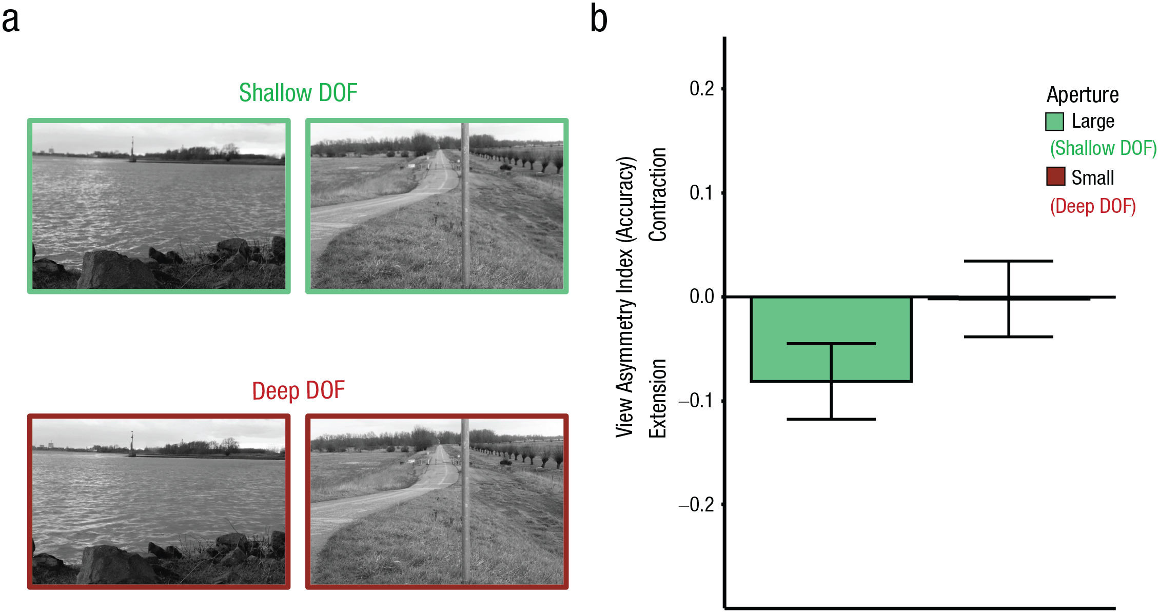
Examples of two scenes from Experiment 4 with shallow and deep depth of field (DOF; a) and results from Experiment 4 (b). For the bar plot (b), the view-asymmetry index was computed as the difference in change-detection accuracy for view changes (close to wide vs. wide to close). Negative values represent higher accuracy in detecting a change from wide to close, indicative of boundary extension. This effect was present for the shallow depth of field and absent for the deep depth of field photographs. Error bars represent standard errors of the mean.

Finally, we generated close-view scenes using the same procedure as in Experiments 2 and 3. Like before, the same scene was resized by an equal percentage across their aperture levels. In total, we had 112 images: 28 for each aperture level in their wide and close views. The masks were generated using the same procedure as in Experiments 2 and 3. The size at which the images were presented was controlled by asking participants to place a real-world object of a standard size (a credit card) on the screen and use it to resize a rectangle displayed on it. On the basis of the ratio between the rectangle image width (in pixels) and the physical width of the card (in millimeters), we scaled the images so that they would appear 15 cm wide and 7.5 cm long on every screen, independently of screen resolution and size. The experiment was conducted online and coded in JavaScript using the jsPsych toolbox (Version 6.2.0; de Leeuw, 2015). The data were saved on the Pavlovia.org servers (www.pavlovia.org).

Design

The experiment consisted of two blocks of 112 trials each. Each block was further divided in four miniblocks of 28 trials each. Within each miniblock, the same scene was not presented more than once. In each miniblock, there were seven scene images for each of the experimental conditions (i.e., two views: close to wide vs. wide to close; two apertures: large vs. small). The second 112-trial block had the same structure as the first block, but the order of the miniblocks was reshuffled. The full design included 224 trials in total.

Procedure

The procedure was the same as in Experiments 2 and 3.

Analyses

The same exclusion criteria as in Experiments 2 and 3 were used. On the basis of these criteria, we excluded two participants because they did not respond on more than 50% of the trials and one participant because their accuracy was 2.5 standard deviations below the group mean across conditions. The analyses included data from 35 participants. As our main analysis, we ran a 2 (view: close to wide vs. wide to close view) × 2 (aperture: large vs. small) repeated measures ANOVA on accuracy.

Results

We found a significant View × Aperture interaction, F(1, 34) = 19.73, p < .001, η_p² = .37 (Fig. 4b). Boundary extension was reliable for the large-aperture condition (M = −0.08, SE = 0.04, 95% CI = [−0.15, −0.01]), t(34) = −2.23, p = .03, d = −0.38, but was no longer observed for the small-aperture condition (M = −0.002, SE = 0.04, 95% CI = [−0.08, 0.07]), t(34) = −0.06, p = .96, d = −0.01, Bayes Factor favoring the null over the alternative hypothesis (BF₀₁) = 5.51. We did not observe a main effect of aperture, F(1, 34) = 1.42, p = .24, η_p² = .04, or a main effect of view change, F(1, 34) = 1.38, p = .25, η_p² = .04. A similar pattern was observed for inverse efficiency scores (RT/% correct), confirming that results were not due to speed/accuracy trade-offs, and for confidence ratings (see the Supplemental Material).

These results generalized the effects of depth of field on boundary extension to a new stimulus set consisting of distant scene views.

General Discussion

In four experiments, we found that boundary extension depends on a photograph’s depth of field. In Experiment 1, across a large and variable image set, depth of field was a strong predictor of boundary extension, with boundary extension being largest for images with shallow depth of field, resembling human vision. By contrast, boundary contraction was only reliably observed for images with deep, unnaturalistic depth of field. Three controlled experiments showed that depth of field modulated boundary extension even when other properties of the scene were kept constant across conditions. Altogether, these results demonstrate that boundary extension is reliably observed for ecologically representative stimuli.

Because depth of field may covary with perceived distance across photographs, we ensured that the relationship between depth of field and boundary extension observed here could not be explained by differences in perceived distance between shallow and deep depth of field. First, in Experiment 1, the relationship between depth of field and boundary extension remained reliable after we regressed out subjective distance ratings. Second, in Experiments 2 and 3, focus distance did not interact with depth of field, even though for large apertures, focus distance was clearly visible (Fig. 2). It should be noted, however, that previous work showed that boundary extension is larger for scenes that show closer compared with faraway views (Bainbridge & Baker, 2020; Bertamini et al., 2005; Hafri et al., 2022; Intraub et al., 1992; Intraub & Dickinson, 2008; Park et al., 2021). These results suggest an additional role for normalization processes. This more generic normalization process (also observed for objects) could exist independently of the more scene-specific predictive mechanism driving boundary extension (Intraub et al., 1996, 1998). Experiment 4 supports this idea, showing no boundary extension for distant scene views with deep depth of field, suggesting that the opposite effects of normalization (leading to boundary contraction) and predictive (leading to boundary extension) processes cancelled each other out for this condition. Importantly, predictive processes were strong for naturalistic (shallow) depth of field, leading to boundary extension even for distant scene views.

When integrating our results with previous findings, we see that the largest boundary extension is observed for photographs with a shallow depth of field taken from a relatively close distance and with the main object seen from a central vantage point (Gagnier et al., 2011). What do all these aspects have in common? One possibility is that images shot under these conditions best resemble how we naturally sample the visual world. Indeed, images with these characteristics show a more partial view of the scene than images with a deep depth of field, wide view, and lateral vantage point. These partial views are more likely to require integration of visual input: When the image is less complete, observers may need to rely more on top-down expectations of scene layout, drawing on sources other than the visual input to complete the percept.

Another aspect that photographs with deep depth of field, shot from a great distance, and shot from a lateral vantage point have in common is that they typically contain many visible objects. To perceptually encode and remember such scenes requires greater attentional resources. This may lead to a loss of peripheral image content, resulting in boundary contraction. Furthermore, fewer resources will be available for predicting what is beyond the scene’s boundaries, thus reducing boundary extension. Nevertheless, our results suggest that the depth-of-field effects on boundary extension observed here cannot be fully accounted for by image complexity. First, the relationship between depth of field and boundary scores remained reliable even when we regressed out the number of objects in the images (see the Supplemental Material). Second, in Experiments 2 and 3, depth of field affected boundary extension regardless of whether the camera’s focus was on the background (showing a larger number of objects) or on the foreground.

Given our results, we propose that boundary extension reflects a constructive mechanism with adaptive value that is conditional to a scene being naturalistic. An image shown at a plausible distance from the observer, with a depth of field resembling the day-to-day perceptual experience, will likely lead to extrapolation of scene layout from memory and, therefore, boundary extension. When one or more of these properties are removed, boundary extension is attenuated. Future research is needed to identify those conditions of the external visual input that allow the mental representation of scenes, stored in memory, to complete external percepts.

By showing stronger boundary extension for images with more naturalistic depth of field, our results support the view that boundary extension is a scene-perception phenomenon rather than a phenomenon specific to photographs (Intraub, 2012). This is in line with previous evidence showing that boundary extension is independent of photographical artifacts (e.g., image magnification; Bertamini et al., 2005) and that it occurs across modalities (Intraub et al., 2015). Nevertheless, the viewing conditions in our experiments differed substantially from our real-world visual experience. Our stimuli were brief static views, did not cover the full visual field, and lacked binocular depth cues, and focus distance was not yoked to the observer’s fixation in the scene. Future studies are needed to test boundary extension for more naturalistic viewing conditions, for example using virtual reality (Snow & Culham, 2021). We predict that boundary extension will be reliably observed under those conditions.

Finally, our results have broad implications for researchers aiming to study natural vision. Many recent psychological, neuroscientific, and computer vision studies implement large stimulus sets to achieve higher ecological validity (e.g., Bainbridge & Baker, 2020; Chang et al., 2019; Hebart et al., 2020; Mehrer et al., 2021). Our findings indicate that such large image sets are not necessarily representative of how observers perceive their visuospatial world. Indeed, there is evidence that decreasing a scene’s realism impacts visual memory (Tatler & Melcher, 2007). By showing that depth of field can drastically change the influence of top-down knowledge on visual processing, our results imply that it is important to use images with naturalistic depth of field in future work.

Supplemental Material

sj-docx-1-pss-10.1177_09567976221140341 – Supplemental material for Predictive Processing of Scene Layout Depends on Naturalistic Depth of Field

Supplemental material, sj-docx-1-pss-10.1177_09567976221140341 for Predictive Processing of Scene Layout Depends on Naturalistic Depth of Field by Marco Gandolfo, Hendrik Nägele and Marius V. Peelen in Psychological Science

Footnotes

Acknowledgements

We thank Surya Gayet, Simen Hagen, Genevieve Quek, and Lu-Chun Yeh for feedback on earlier versions of this article and the other Peelen Lab members for helpful discussions and feedback during lab meetings.

Transparency

Action Editor: Sachiko Kinoshita

Editor: Patricia J. Bauer

Author Contributions

Marco Gandolfo: conceptualization, data curation, formal analysis, investigation, methodology, resources, software, visualization, writing – original draft, writing – review & editing.

Hendrik Nägele: resources.

Marius V. Peelen: conceptualization, funding acquisition, methodology, supervision, writing – review & editing.

ORCID iD

Marco Gandolfo

Supplemental Material

Additional supporting information can be found at

References

Artal

(2014). Optics of the eye and its impact in vision: A tutorial. Advances in Optics and Photonics, 6(3), 340–367.

Bainbridge

W. A.

Baker

C. I.

(2020). Boundaries extend and contract in scene memory depending on image properties. Current Biology, 30(3), 537–543.

Barthelmé

Tschumperlé

(2019). imager: An R package for image processing based on CImg. Journal of Open Source Software, 4(38), Article 1012. https://doi.org/10.21105/joss.01012

Bartlett

F. C.

(1932). Remembering: A study in experimental and social psychology. Cambridge University Press.

Bertamini

Jones

L. A.

Spooner

Hecht

(2005). Boundary extension: The role of magnification, object size, context, and binocular information. Journal of Experimental Psychology: Human Perception and Performance, 31(6), 1288–1307.

Brady

T. F.

Konkle

Alvarez

G. A.

(2011). A review of visual memory capacity: Beyond individual items and toward structured representations. Journal of Vision, 11(5), Article 4. https://doi.org/10.1167/11.5.4

Chang

Pyles

J. A.

Marcus

Gupta

Tarr

M. J.

Aminoff

E. M.

(2019). BOLD5000, a public fMRI dataset while viewing 5000 visual images. Scientific Data, 6(1), Article 49. https://doi.org/10.1038/s41597-019-0052-3

de Leeuw

J. R

. (2015). jsPsych: A JavaScript library for creating behavioral experiments in a Web browser. Behavior Research Methods, 47(1), 1–12.

Dickinson

C. A.

Intraub

(2008). Transsaccadic representation of layout: What is the time course of boundary extension? Journal of Experimental Psychology: Human Perception and Performance, 34(3), 543–555.

10.

Eaton

J. W.

Bateman

Hauberg

(1997). Gnu Octave (Version 5.1.0) [Computer software]. https://octave.org/

11.

Gagnier

K. M.

Intraub

Oliva

Wolfe

J. M.

(2011). Why does vantage point affect boundary extension? Visual Cognition, 19(2), 234–257.

12.

Gottesman

C. V.

Intraub

(2002). Surface construal and the mental representation of scenes. Journal of Experimental Psychology: Human Perception and Performance, 28(3), 589–599.

13.

Hafri

Wadhwa

Bonner

M. F.

(2022). Perceived distance alters memory for scene boundaries. Psychological Science, 33(12), 2040–2058.

14.

Hebart

M. N.

Zheng

C. Y.

Pereira

Baker

C. I.

(2020). Revealing the multidimensional mental representations of natural objects underlying human similarity judgements. Nature Human Behaviour, 4(11), 1173–1185.

15.

Hecht

(1987). Optics (2nd ed.). Addison-Wesley.

16.

Hubbard

T. L.

Hutchison

J. L.

Courtney

J. R.

(2010). Boundary extension: Findings and theories. Quarterly Journal of Experimental Psychology, 63(8), 1467–1494.

17.

Intraub

(2010). Rethinking scene perception: A multisource model. In Ross

B. H.

(Ed.), The psychology of learning and motivation (Vol. 52, pp. 231–264). Academic Press.

18.

Intraub

(2012). Rethinking visual scene perception. Wiley Interdisciplinary Reviews: Cognitive Science, 3(1), 117–127.

19.

Intraub

(2020). Searching for boundary extension. Current Biology, 30(24), R1463–R1464.

20.

Intraub

Bender

R. S.

Mangels

J. A.

(1992). Looking at pictures but remembering scenes. Journal of Experimental Psychology: Learning, Memory, and Cognition, 18(1), 180.

21.

Intraub

Dickinson

C. A.

(2008). False memory 1/20th of a second later: What the early onset of boundary extension reveals about perception. Psychological Science, 19(10), 1007–1014.

22.

Intraub

Gottesman

C. V.

Bills

A. J.

(1998). Effects of perceiving and imagining scenes on memory for pictures. Journal of Experimental Psychology: Learning, Memory, and Cognition, 24(1), 186–201.

23.

Intraub

Gottesman

C. V.

Willey

E. V.

Zuk

I. J.

(1996). Boundary extension for briefly glimpsed photographs: Do common perceptual processes result in unexpected memory distortions? Journal of Memory and Language, 35(2), 118–134.

24.

Intraub

Morelli

Gagnier

K. M.

(2015). Visual, haptic and bimodal scene perception: Evidence for a unitary representation. Cognition, 138, 132–147.

25.

Intraub

Richardson

(1989). Wide-angle memories of close-up scenes. Journal of Experimental Psychology: Learning, Memory, and Cognition, 15(2), 179–187.

26.

Konkle

Oliva

(2007). Normative representation of objects: Evidence for an ecological bias in object perception and memory. In Proceedings of the Annual Meeting of the Cognitive Science Society (Vol. 29, pp. 407–412). Cognitive Science Society.

27.

Kuznetsova

Rom

Alldrin

Uijlings

Krasin

Pont-Tuset

Kamali

Popov

Malloci

Kolesnikov

Duerig

Ferrari

(2020). The Open Images dataset V4. International Journal of Computer Vision, 128(7), 1956–1981.

28.

Maguire

E. A.

Mullally

S. L.

(2013). The hippocampus: A manifesto for change. Journal of Experimental Psychology: General, 142(4), 1180–1189.

29.

McDunn

B. A.

Siddiqui

A. P.

Brown

J. M.

(2014). Seeking the boundary of boundary extension. Psychonomic Bulletin & Review, 21(2), 370–375.

30.

Mehrer

Spoerer

C. J.

Jones

E. C.

Kriegeskorte

Kietzmann

T. C.

(2021). An ecologically motivated image dataset for deep learning yields better models of human vision. Proceedings of the National Academy of Sciences, USA, 118(8), Article e2011417118. https://doi.org/10.1073/pnas.2011417118

31.

Middleton

W. E. K.

(1957). Vision through the atmosphere. In Bartels

(Ed.), Geophysik II [Geophysics II] (pp. 254–287). Springer.

32.

Park

Josephs

E. L.

Konkle

(2021, January 26). Systematic transition from boundary extension to contraction along an object-to-scene continuum. Psyarxiv Preprints. https://doi.org/10.31234/osf.io/84exs

33.

Park

Intraub

D.-J.

Widders

Chun

M. M.

(2007). Beyond the edges of a view: Boundary extension in human scene-selective visual cortex. Neuron, 54(2), 335–342.

34.

R Core Team. (2020). R: A language and environment for statistical computing (Version 4.0.1) [Computer software]. https://www.R-project.org/

35.

Snow

J. C.

Culham

J. C.

(2021). The treachery of images: How realism influences brain and behavior. Trends in Cognitive Sciences, 25(6), 506–519.

36.

Tatler

B. W.

Melcher

(2007). Pictures in mind: Initial encoding of object properties varies with the realism of the scene stimulus. Perception, 36(12), 1715–1729.

37.

Willenbockel

Sadr

Fiset

Horne

G. O.

Gosselin

Tanaka

J. W.

(2010). Controlling low-level image properties: The SHINE toolbox. Behavior Research Methods, 42(3), 671–684.

38.

Xiao

Ehinger

K. A.

Hays

Torralba

Oliva

(2016). SUN database: Exploring a large collection of scene categories. International Journal of Computer Vision, 119(1), 3–22.

Supplementary Material

Please find the following supplemental material available below.

For Open Access articles published under a Creative Commons License, all supplemental material carries the same license as the article it is associated with.

For non-Open Access articles published, all supplemental material carries a non-exclusive license, and permission requests for re-use of supplemental material or any part of supplemental material shall be sent directly to the copyright owner as specified in the copyright notice associated with the article.

0.00 MB

8.72 MB