
Abstract
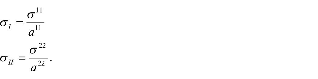
The formfinding of shell, masonry vault and fabric or cable net structures involves obtaining a geometry and a stress state in equilibrium under a dominant load case. In so doing we can give the formfinding model very different properties to those of the finished structure, for example modelling a fabric structure by a soap film. In order to obtain a formfound geometry we need to make a number of decisions about the geometrical and structural properties we aim to achieve. These decisions can be couched in a number of ways, and in this paper we concentrate on statements about the principal curvatures of the surface and the principal membrane stresses. A Weingarten surface has a functional relationship between the mean of the two principal curvatures and their product – the Gaussian curvature. Examples include minimal surfaces, surfaces of constant mean curvature and surfaces of constant Gaussian curvature. It is well known that the Codazzi equations enable us to obtain a spacing of the principal curvature lines on a Weingarten surface that is not arbitrary, but determined by the principal curvatures. The Codazzi equations are purely geometric but they are identical with the in plane components of the membrane equilibrium equations for the case when there is no tangential load. Zero-length or close-coiled springs are used in the Anglepoise lamp and have a length that is proportional to the tension, once the tension is sufficient for the coils to separate. We demonstrate that surfaces constructed from a fine grid of zero-length springs have a membrane stress such that the product of the principal stress is constant. If we add an isotropic stress we arrive at a condition similar to that for the curvature of a linear Weingarten surface. We provide a number of examples of the application of these ideas.
Keywords
Introduction
The formfinding of shell, masonry vault and fabric or cable net structures involves obtaining a geometry and a state of stress in equilibrium under a dominant load case. In so doing we can give the formfinding model – either a physical or a numerical model – very different properties to those of the finished structure. Modelling a fabric structure by a soap film is the best known example.1,2 Other possibilities include modelling a masonry structure by a hanging stretchy latex rubber or Lycra model loaded with weights, which we then invert to form a masonry structure in compression.3,4 Similarly a hanging chain model can be inverted to give the shape of a timber gridshell. 5 Slender timber structures may be subject to creep deformation, and so even though timber gridshells are lightweight structures, the permanent own weight load can be more important than short term wind and snow loads. Slender timber structures are subject to the possibility of creep buckling, 6 which is particularly difficult to predict because of the lack of data on the rate of creep and how it is influenced by stress, moisture content and so on. Essentially creep deformation increases the imperfections in the geometry of the structure, which may in turn reduce the buckling load.
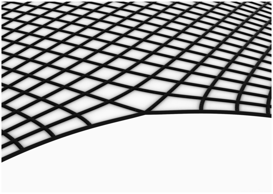
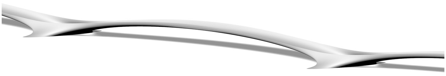
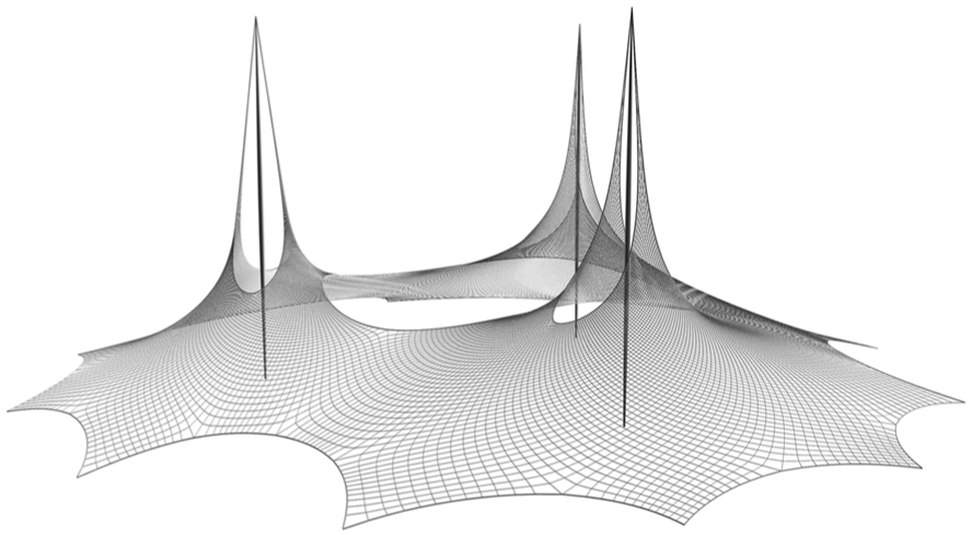
Our aim in pursuing this work was to produce designs for a shell such as that in Figure 1, which has two large openings. It would be usual in the design of such a shell to introduce edge arches or stiffeners, and so concentrate forces into the boundary. However, in certain situations it might be preferable to have a more even distribution of stress and hence avoid unsightly edge members. In aiming for this we were very much influenced by the physical models of Heinz Isler, 4 in particular obtaining the upturned lip at the edge of the shell.
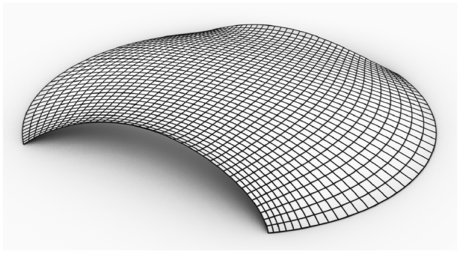
Inverted hanging shell. When hanging the zero-length springs shown in black are in tension balancing the own weight of the shell and an isotropic surface compression varying with height reducing away from the support, balancing the tangential component of the hanging weight. The net stress in the hanging model is always tensile and the isotropic compressive stress balances the tension in the zero-length springs at the boundary in the direction normal to the boundary. This model has tension coefficients that are independent of time, but do vary with position on the surface.
The distribution of forces in a shell, tension structure or masonry vault is influenced by the structural grid or pattern of masonry blocks and vice versa. And so we are very interested in the arrangement of the grid and its relationship with the curvature of the structure and the stress distribution. This means that we are equally concerned with structural and geometric equations, and have to ensure that we use the same mathematical notation for them both.
Fundamentals of the formfinding of shells and the contributions in this paper
Even though shell structures almost invariably experience internal bending moments under applied loads, such as wind or snow, the aim in the formfinding process is to make the structure work by membrane action under some idealised dominant load case. Membrane action means tensions and compressions in the local tangent plane to the surface with no bending moments or shear forces normal to the surface (Figures 1–5).
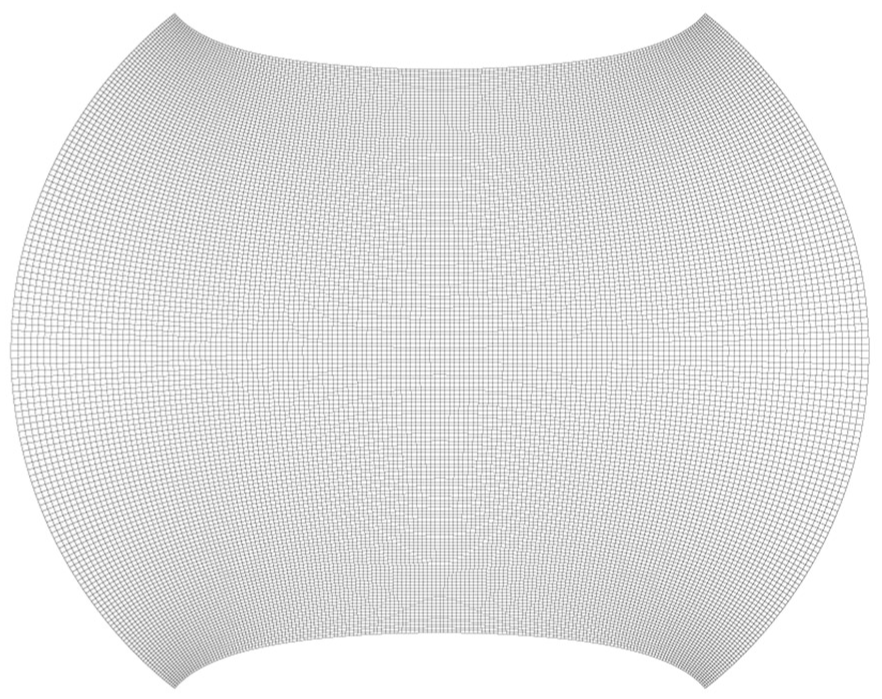
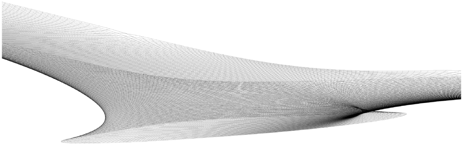
Structural grid of the shell in Figure 1.The grid in Figure 1 is drawn coarser in order to show the zero-length springs clearly. The analysis took approximately 15 s to converge on a 2017 MacBook Air using a program written using the Processing https://processing.org programming environment.
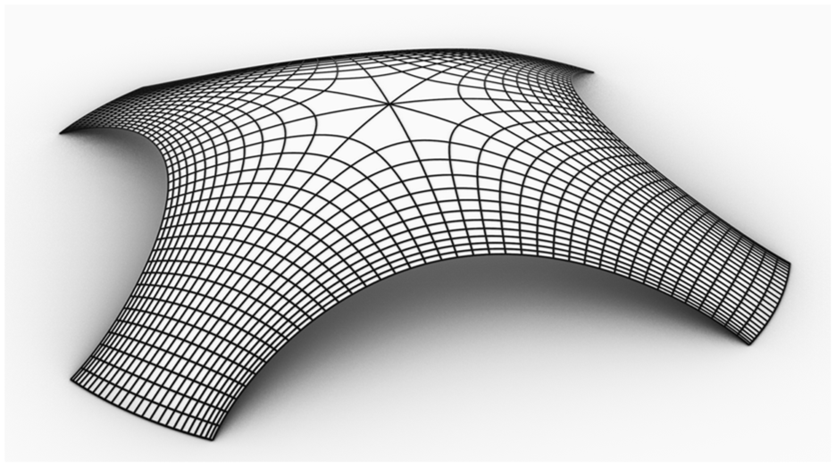
Inverted hanging shell of the same type as that in Figure 1, but with four openings. This model does have the same tension coefficient at all points on the surface. The longer springs have a higher tension, but they also have a higher spacing, so that membrane stress is approximately constant away from the boundaries.
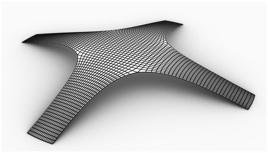
Inverted hanging shell of the same type as that in Figure 3, but with a different grid. This model does have the same tension coefficient at all points on the surface. The area of longer springs is moved from the centre of the shell in Figure 3 to the mid-points of the boundaries, as shown in detail in Figure 5.
Detail of shell in Figure 4.
In the formfinding of structures the geometry is treated as an unknown. However, before discussing that it is worth considering the simpler case of when the geometry is known. The membrane theory of shells has equilibrium equations in three directions and three unknown components of membrane stress. We therefore have the same number of equations as unknowns, if we know the shape of the shell and the loading upon it. The three equations can be reduced to one partial differential equation which is elliptic if the Gaussian curvature is positive and hyperbolic if the Gaussian curvature is negative. 7 This means that shells with positive Gaussian curvature and negative Gaussian curvature behave very differently, and require different boundary support to be statically determinate, and avoid being mechanisms. There are a number of ways to reduce the three equations of equilibrium to one equation, 8 and the simplest way is to derive Puchers equation which is described in §113 of Timoshenko and Woinowsky-Krieger. 7
In formfinding we generally reverse the problem and specify certain properties of the state of stress and the geometry is treated as an unknown. The problem will be elliptic if the shell is all in tension or all in compression and hyperbolic if the product of the principal membrane stress is negative. However, in some cases we might impose a mixture of geometric and stress constraints and we have to be careful to ensure that we have sufficient constraints for the problem to be determinate, but not too many constraints so that there is no solution.
In specifying the geometry we need the shape of the surface representing the structure, but also the geometry of the structural grid which might represent members of a gridshell or the stone blocks of a vault. 9
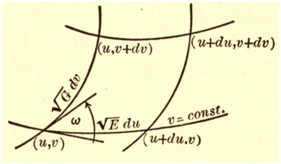
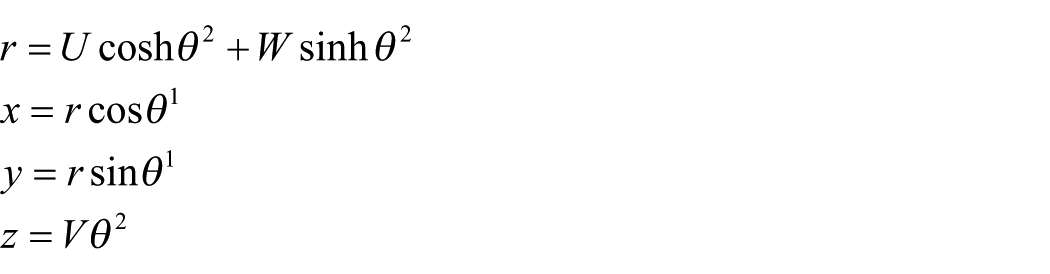
We define the position of a point on a surface using surface coordinates or parameters. Traditionally these coordinates are chosen to be
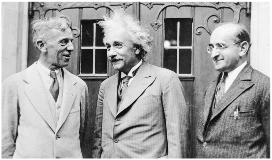
Albert Einstein with two of his colleagues at Princeton University in 1933, Luther Eisenhart on the left and Walther Mayer on the right.
In general it is convenient to align the structural grid with the coordinate grid and we shall do this. However, there might be circumstances when they are not aligned, in which case we have essentially two coordinate systems, and the tensor notation is particularly suited to a change of coordinate system.
The tensor notation that we shall be using for differential geometry is described in detail in Appendix A and the structural equations that we need are derived in Appendix B, which includes bending moments. The reason for this is that a proper understanding of the membrane theory is best achieved by treating it as a special case of the bending theory.
The unknowns that we have to deal with are the geometric quantities
Next we have the
Finally we have the components of the symmetric membrane stress tensor. Green & Zerna use
The components of the first and second fundamental forms must satisfy the Gauss-Codazzi equations,
14
that is Gauss’s Theorema Egregium and the Peterson-Mainardi-Codazzi equations. The Gauss-Codazzi equations are three partial differential equations. In addition we have the equilibrium equations, so that we have six equations and nine unknowns,
Thus we need three more equations to perform formfinding. For a prestressed or hanging equal mesh or Tchebychev
15
net we have the shear stresses component
For a fabric structure based on a soap film we have the mean curvature
if
However the easiest way to ensure
Thus in both these simple cases formfinding involves making a mixture of three geometric and structural statements. We can, of course make just one statement to define a surface, perhaps in the Monge form
An elastic membrane is one in which there is a relationship between the membrane stress components
In formfinding we are free to choose
A hyperelastic or Green elastic sheet is a sheet whose stress-strain relationship derives from a strain energy density function.19,20 The Green strain energy function is named after George Green (1793–1841) 21 who should not be confused with Albert Edward Green (1912–1999).11,20 A Cauchy elastic material 19 is a material in which the stress is a unique function of the strain, but which does not admit a strain energy density function, although quite how such a material could exist without breaking the first law of thermodynamics is unclear.
We shall assume that we have a Green elastic material, and purely geometric constraints, such as constant lengths or geodesics, which correspond to allowing some stiffnesses to tend to infinity. The constraints then become Lagrange multipliers which can be simply included as unknowns in the relaxation process, including a rate of change of the Lagrange multipliers. If a cable of an equal mesh net is too long we increase the tension, if it is too short we reduce the tension, and we can, if we are so minded, include the rate of change of tension as a damped variable.
A soap film is an elastic membrane in which the strain energy per unit area is a constant equal to the isotropic surface tension. Hence minimising the surface area and minimising the strain energy are identical problems.
A particularly useful hyperelastic sheet is a continuum made from a very large number of zero-length or close-coiled springs that have a length that is proportional to the tension, once the tension is sufficient for the coils to separate. Figure 8(a) shows the tension / length relationship for a zero-length spring. The coils touch when unloaded and only when a certain tension is reached do they begin to separate in such a way that thereafter the tension is proportional to the length. Thus, even though the springs do not have a zero length when unstressed, we use the term zero-length spring to mean a spring with a linear length/tension relationship which can be extrapolated back to the origin.
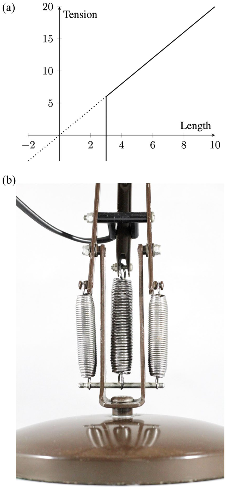
Zero-length springs: (a) length/tension relationship for zero-length spring and (b) springs of an Anglepoise lamp. Image: TheGoodEndedHappily, CC BY-SA 4.0.
It would seem that the practical manufacture of zero-length springs was pioneered independently by George Carwardine 22 for use in the Anglepoise lamp (Figure 8(b)) and Lucien LaCoste 23 for use in gravimeters.
The terms tension coefficient and force density were coined by Southwell 24 and Linkwitz and Schek,25 –27 respectively, to mean the tension in a structural element divided by its length. Therefore we can describe a zero-length spring as a member with constant tension coefficient or force density.
We shall demonstrate that the product of the two principal membrane stresses remains constant as a zero-length spring surface is deformed.
We can draw a principal curvature line on a surface by starting at an arbitrary point and moving backwards or forwards in one of the two principal curvature directions. This involves solving the eigenvalue-eigenvector problem 14
in which the eigenvalues,
We can draw a number of principal curvature lines by starting at a number of arbitrary points, and the spacing of the principal curvature lines is arbitrarily determined by the starting points.
A Weingarten surface is one in which there is a functional relationship between the mean and Gaussian curvatures, and it is well known 10 that the Codazzi equations enable us to obtain a spacing of the principal curvature lines on a Weingarten surface that is not arbitrary, but determined by the principal curvatures.
A linear Weingarten surface has a linear relationship between the mean and Gaussian curvatures and examples include minimal surfaces, surfaces of constant mean curvature and surfaces of constant Gaussian curvature.
It is less well known that in the absence of tangential loads on a shell working by membrane action, the equilibrium equations in the tangential directions are identical to the Codazzi equations, and hence the spacing of the principal membrane stress lines is uniquely determined, provided that we have a functional relationship between the mean and product of the two principal membrane stresses.
If we add an isotropic tension or compression to the zero-length spring membrane stress we arrive at the same condition for membrane stress as we do for curvature of a linear Weingarten surface. Thus the results for linear Weingarten surface can be applied directly to the spacing of the principal membrane stress trajectories, which are important for structural design. In general the principal curvature directions and the principal membrane stress directions do not coincide, unless this is imposed as a constraint.
It is ‘conventional’ in the design of shell structures to have a relatively ‘flimsy’ shell supported on ‘substantial’ edge beams, arches and cables. One of the aims of this work is to formfind shapes in which the forces that would have been concentrated in the edge beams or arches are distributed into the shell itself, more like the shells that we see in nature. 28
We demonstrate that under certain conditions an isotropic hyperelastic sheet will have such a functional relationship between the mean and product of the two principal membrane stresses.
We use a large number of ‘standard results’ which are relegated to appendices, as described above. Many of these results are found in Green and Zerna, 11 in Green and Adkins 20 or in Eisenhart, 10 but not always in a form suitable for our use, or derived in a manner consistent with our narrative. The book Pinkall and Gross 29 Differential Geometry: From Elastic Curves to Willmore Surfaces is interesting because it covers essentially what we would call the bending theory of shells, but without mentioning concepts such as ‘force’, ‘moment’, ‘stress’ or ‘tensor’.
Comparison with existing methods of formfinding
In order to discuss existing methods of formfinding it is helpful to divide the process into three parts:
Define a conceptual model involving geometrical and structural quantities. If the model is a continuum model this will involve differential equations or the minimisation of surface integrals. If the model is discrete the equations will be simultaneous equations which are often non-linear.
Examples of such conceptual models include the Force Density Method, 25 Thrust Network Analysis, 30 Membrane Equilibrium Analysis 31 and the use of machine learning. 32 The force density method allows one to treat the elements of a cable net as inextensional in which case the tensions in an element can no longer be calculated from the strain and instead the force densities or tension coefficients are treated as additional unknowns.
2. For a numerical solution a continuum model has to be converted to a discrete model. This almost invariably involves use of the finite element method, and other methods, such as the finite difference method can be considered as special cases of the finite element method with appropriate shape functions. Particle methods, such as smoothed particle hydrodynamics and peridynamics can be considered as the use of finite elements which overlap and merge into each other. Isogeometric analysis is the use of finite element shape functions borrowed from computer aided design, including NURBS 33 and Bézier triangles. 34
3. Numerical solution of the equations. Here the techniques can be broadly described as implicit matrix methods or explicit relaxation methods. Since the equations are often non-linear, matrix methods may involve techniques such as Newton-Raphson. Relaxation techniques were introduced by Southwell 35 include Verlet integration 17 and dynamic relaxation, 18 which is effectively Verlet integration applied to a static problem, leading to a damped oscillation about the equilibrium state.
From an engineering point of view it does not matter whether matrix or relaxation techniques are used to solve the equations, and the equations produced by the finite element method can equally well be solved using either technique. The Force Density Method 25 uses matrices, but the equations could equally well be solved using relaxation.
Those who are so minded can write their own software using, for example C++ and OpenGL, or Processing https://processing.org. Alternatively they or they can use an environment such as Daniel Piker’s Kangaroo3d http://kangaroo3d.com in Rhino Grasshopper.
Principal stress trajectories
The stress in a membrane is a symmetric second order tensor, in exactly the same way that curvature of a surface can be described by a symmetric second order tensor. This means that we have orthogonal principal membrane stresses just as we have orthogonal principal curvatures. In the from finding process we are interested in both the principal stress directions and the principal curvature directions, and we may align structural members and cladding panels either with the stresses or the curvatures. Ideally we would align the principal curvatures and the principal stresses, but this may be difficult.
In the same way that we can plot principal curvature directions we can plot the principal stress trajectories by starting at some arbitrary point and then solving the eigenvalue problem to move in one of the principal directions. The arbitrary starting points mean that the spacing of the curves on the surface is not well controlled. We shall show that if we put conditions corresponding to those for a Weingarten surface on the state of membrane stress in a structure, then the principal stress trajectories become controlled, and the numerical procedure automatically produces principal stress trajectories as shown in Figures 3, 4, 9 and 10.
Inverted hanging bridge entirely in compression under own weight and a hydrostatic pressure to model internal fill supporting the roadway. The zero-length springs in the model all have the same constant tension coefficients.
Detail of bridge in Figure 9 showing structural grid.
The structural theory for membrane stress and the geometric theory for curvature are essentially the same. However one can do geometry with no knowledge of structures, but one can not do structures with no knowledge of geometry, so it would seem simpler to start with geometry and Weingarten surfaces.
Weingarten surfaces
A Weingarten surface is a surface for which there is a functional relationship between the mean and Gaussian curvature.36,37 The mean curvature is the mean of the two principal curvatures and the Gaussian curvature is the product of the principal curvatures. Eisenhart
10
calls Weingarten surfaces
or
Thus, writing
where
which is equation (45) in Article 123 of Chapter VIII of Eisenhart.
10
He then points out that if we have a functional relationship between
where
In the case of a minimal surface for which
so that we obtain the well known result that

which appears in Article 109 in Chapter VII of Eisenhart. 10
Linear Weingarten surface
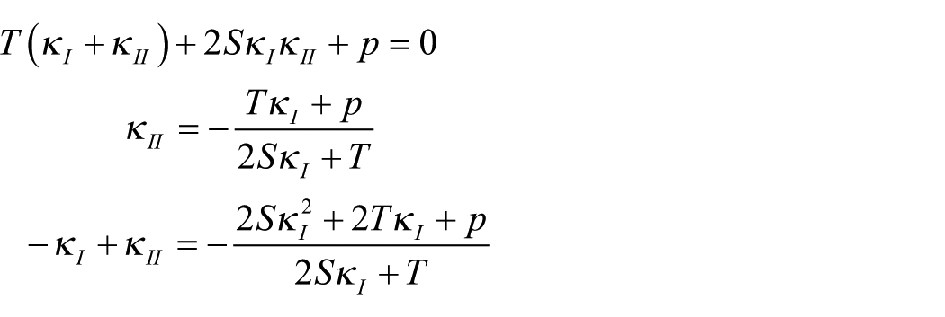
A linear Weingarten surface10,36,37 is a surface which satisfies the relationship

where
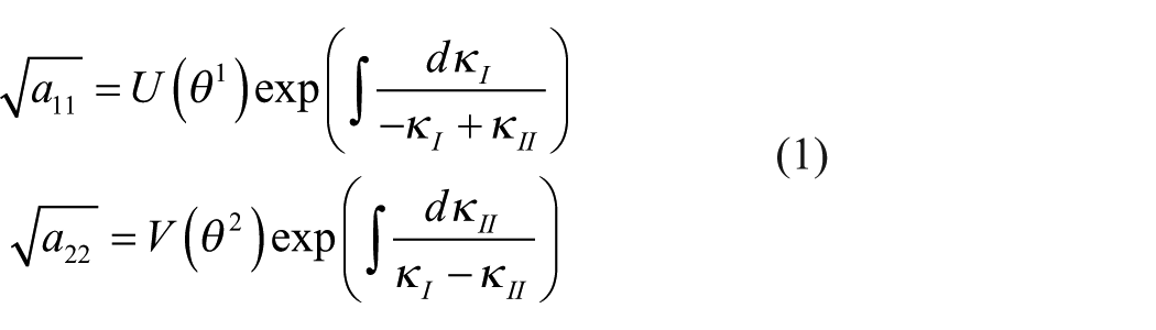
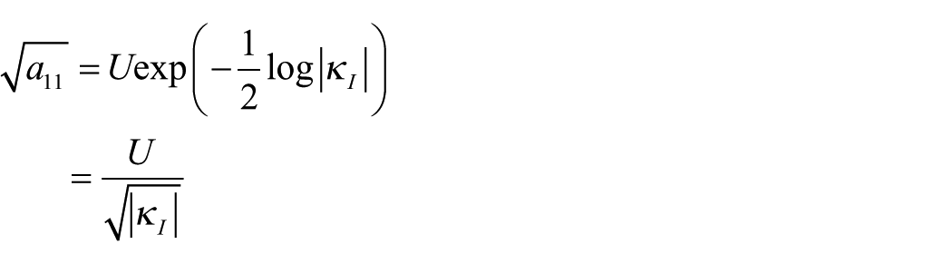
We have from (2) or (D4),
so that
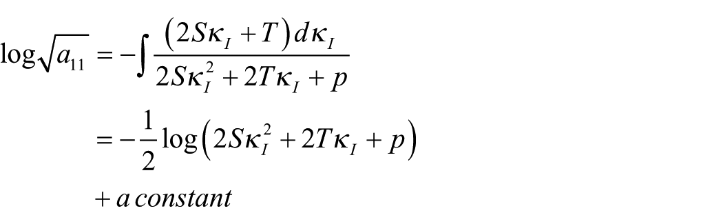
and
where
and again
On the other hand, if
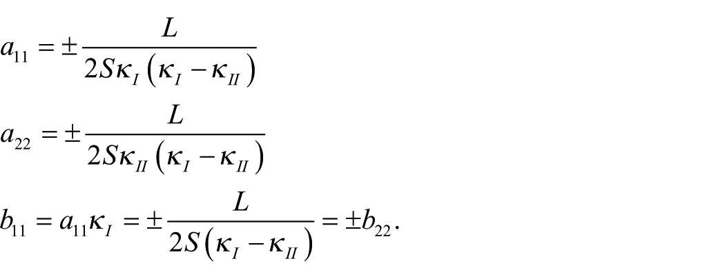
which means that the diagonals of the principal curvature coordinates form a Tchebychev net. Using 2, the product
Thus, we arrive at the conclusion that principal curvature coordinates on a linear Weingarten surface can be constructed such that
If
If
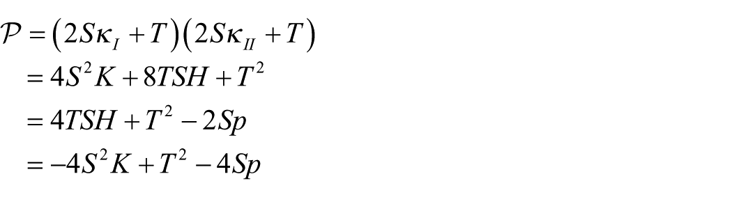
The curvature and twist in the directions of the diagonals of the principal curvature net are
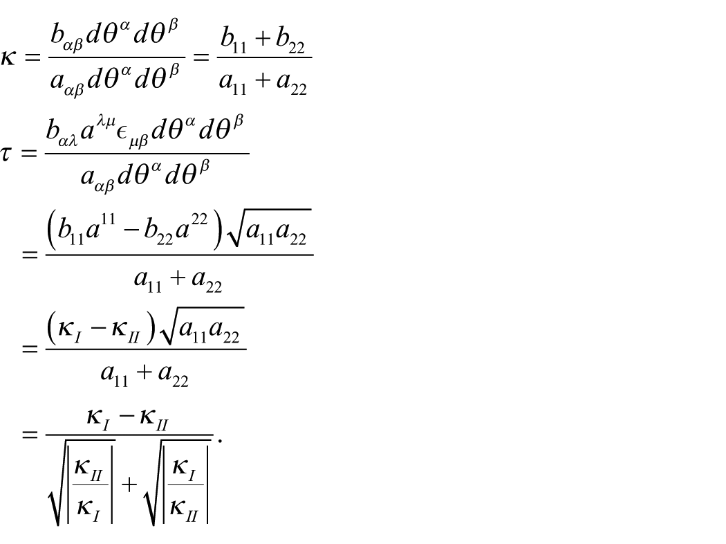
If
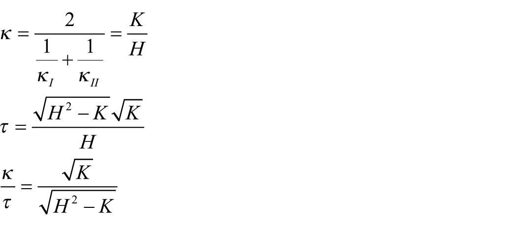
so that a line through the origin is tangent to the Mohr’s circle of curvature
39
at the point
We demonstrate in Appendix D how a linear Weingarten surface can be obtained by the minimisation of a surface integral, which could represent strain energy. We have relegated this to an appendix since it involves the bending theory, introduced in Appendix B and since we have introduced the bending theory, we describe the Willmore surface in Appendix E.
Boundary conditions at a free edge
Tellier et al. 37 discuss the boundary condition for a linear Weingarten surface attached to a cable, but here we will consider the case when we have a free edges with no forces applied to it. The normal shear force is automatically zero from (D1), leaving us with the membrane stresses in (D2) and (D3).
Consideration of Mohr’s circle of stress
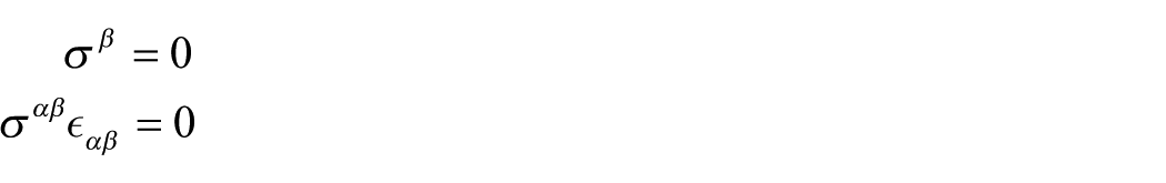
40
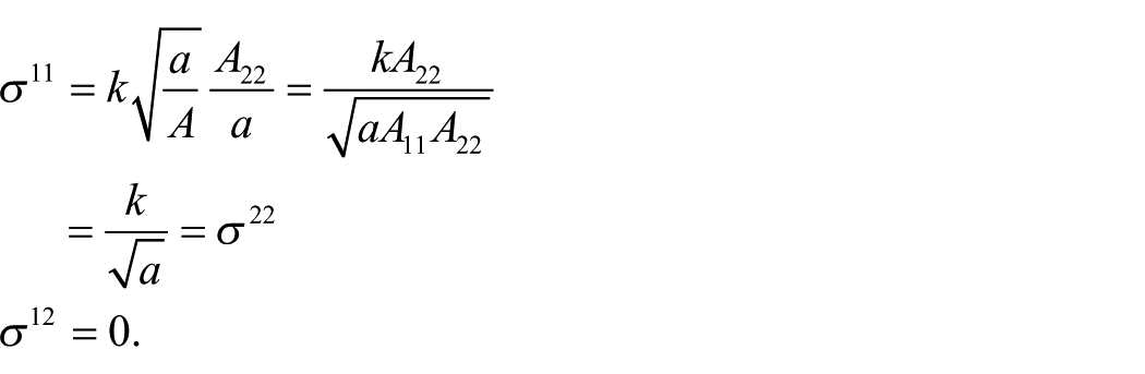
tells us that a free edge must be in a principal stress direction and that that principal stress must be zero. Thus, if we take

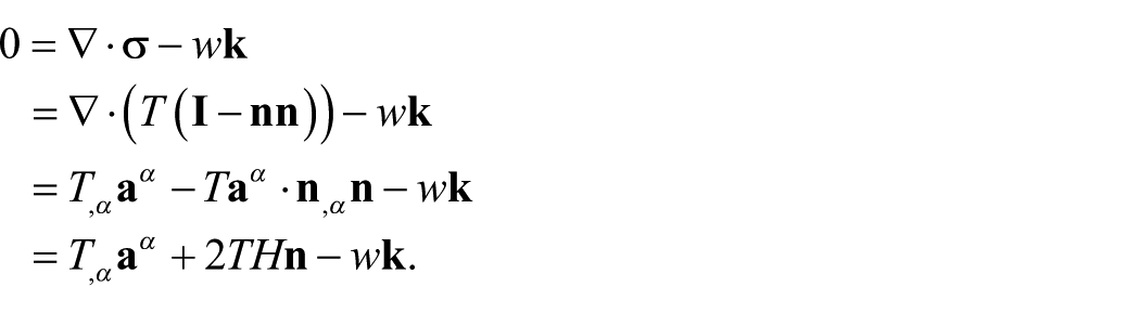
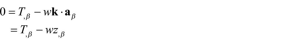
The membrane equilibrium equations
The equation of equilibrium of forces for shells in both the membrane and bending theories is (B2), repeated here

where
In the membrane theory there are no bending moments or normal shear forces and so (B3) become
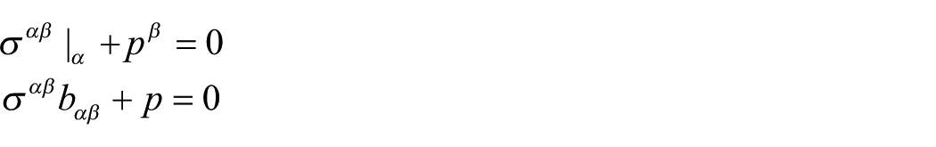
and (B4) become
so that
In the case when there are no tangential loads, then

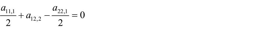
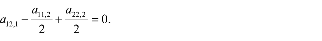
Now we can rewrite the Codazzi equations (A12) as
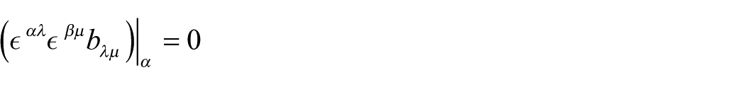
which is exactly the same as (4) if we replace the tensor with components
The tensor with components
This means that the results (1) from the Codazzi equations become
if the coordinates follow the principal membrane stress directions and we have a functional relationship between
Isotropic hyperelastic membrane
In Appendix C we derive (C8) which we repeat here,
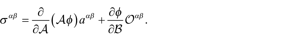
The tensor
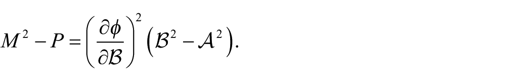
The mean
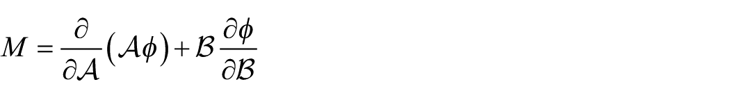
and
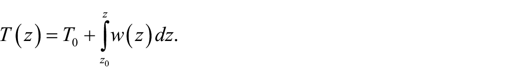
A soap film subject to its own weight
Minimal surfaces are of great interest to mathematicians 41 and to architects and engineers, notably Frei Otto 42 and Sergio Musmeci,43,44 for the finding of beautiful and efficient structural forms. Minimal surfaces minimise the area of a surface, and this is the same as minimising the strain energy of a weightless surface with a constant strain energy per unit area, corresponding to a homogeneous isotropic surface tension. Soap films are not weightless, and so cannot be in equilibrium with uniform surface tension. It would seem reasonable to assume that the surface tension in a soap is isotropic, that is that it has the same value in all directions at a particular point, since otherwise there would be shear stresses in the film. However the surface tension clearly cannot be homogeneous since the tension at the top of a vertical soap film must be greater than that at the bottom to balance the weight of the film. In addition, for stability the surface tension must increase where the film is thinner to pull more fluid back into a thin region. 45 This is the reverse of gas pressure increasing with density. The variation in soap film thickness can be seen from the thin-film interference patterns in Figure 11.
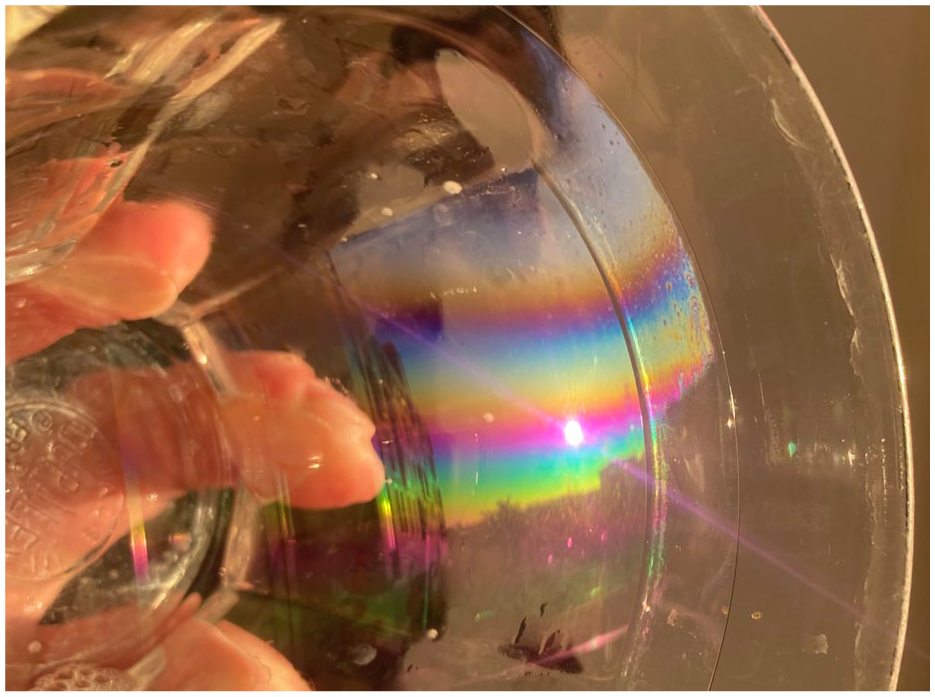
Thin-film interference on a soap film in a drinking glass
We are thus interested in the variation of stress in a soap film, which can be related to the strain energy per unit area stored in the film. If one watches a soap film one can see that the fluid is not stationary and is continuously in motion. ’Material points’ are free to move on the surface and the surface tension can only depend on the thickness of the film. The film carries no memory of the shape it may have been in the past, it has no understanding of the concept of strain.
If the stress is isotropic,
in (C8) to give
where the surface tension,
If write
where
Thus for equilibrium in the normal direction

and in the tangential direction,
where
Thus the gradient
Zero-length spring surfaces
Let us write
where
Then, from (C8)
and from (C9) and (C10),
Therefore
Now let us for simplicity examine the case when
We have
and therefore
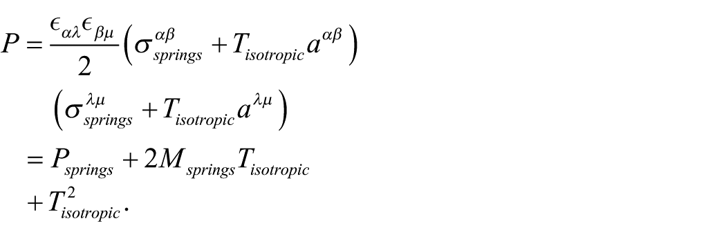
The components of membrane stress,
and the product of the two principal membrane stresses is equal to

Thus as the membrane is deformed and strained, the product of the two principal membrane stresses remains constant at any point moving with the surface, although it may vary from point to point.
One might imagine that it is not possible to make a real physical surface with this interesting property, but we shall see that it can be done, at least in theory by making the surface from a fine grid of zero-length springs, each carrying a tension sufficient for the coils to separate. We described zero-length springs earlier in this paper and Figure 8(a) shows the tension / length relationship for a zero-length spring.
Perhaps the most important property of zero-length springs or constant tension coefficient members is that if the member is projected onto a plane, the member in the plane has the same tension coefficient. This is because the component of length and the component of force are both resolved in the same way.
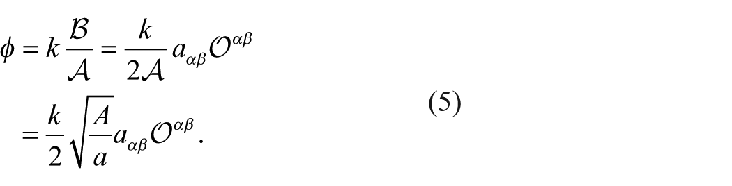
The strain energy in a zero-length spring is equal to a the spring stiffness times half its length squared plus a constant. However we are not interested in this constant since we are always interested only in the change of strain energy. Now let us imagine that we have constructed a membrane from some fine grid of zero-length springs. The square of the distance between two points on a surface is equal to
However from (5) the strain energy contained within a parallelogram of sides
These two expressions are identical in that they both involve a summation of
Thus we can say that a surface made of a fine grid of zero-length springs produces a membrane in which the product of the principal stresses remains constant as the membrane is stretched in any direction. This product may vary with position as given by the surface coordinates, which are convected with the membrane. This applies regardless of the grid pattern of the springs, which might be triangular, quadratic, hexagonal or even a random array of springs as shown in Figure 12.
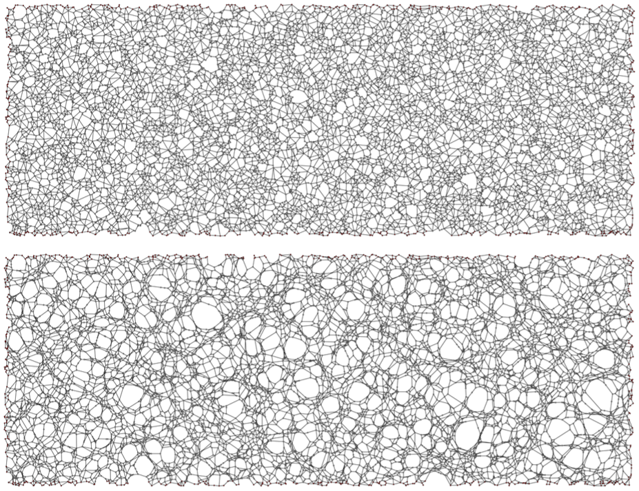
Random grid before and after relaxation. The initial grid consists of a random array of points joined by a Gabriel graph. 46
Properties of an unloaded homogeneous zero-length spring surface
If the surface is unloaded, then
If we replace

so that we have a constant isotropic surface tension. Let us choose a coordinate system in the reference configuration such that
The fact that
We can write the equilibrium equation (B2) as
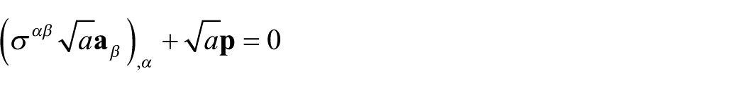
so, if
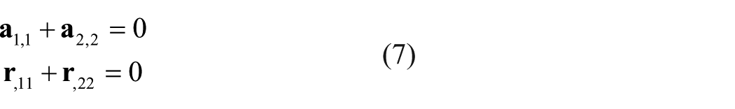
or in Cartesian coordinates
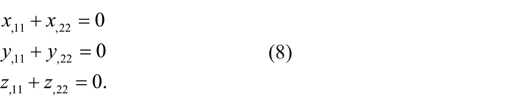
Thus the Cartesian coordinates satisfy Laplace’s equation as a function of the surface coordinates.
In the case of radial symmetry, the solution to (8) is simply
where
and if we scalar multiplying the same equation by
Thus
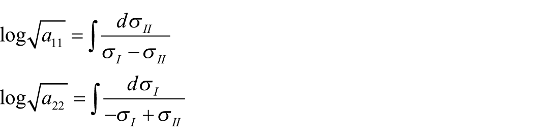
so that
and

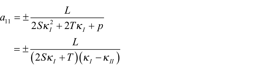
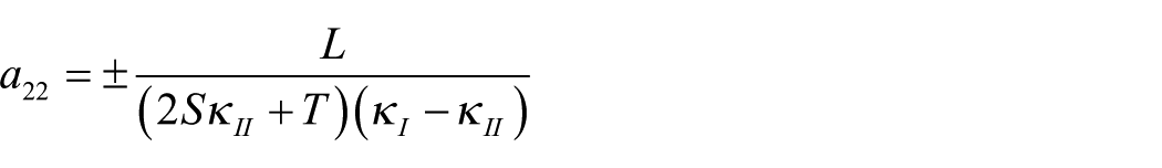
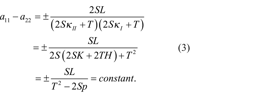
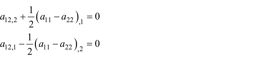
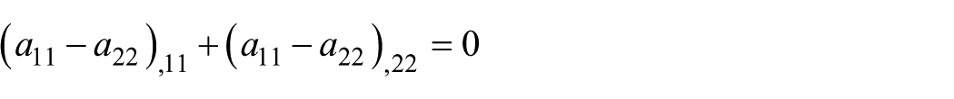
Thus both (a11 – a22) and a12 satisfy Laplace’s equation. This means that if we arrange the boundary conditions such that a12 = 0 all around the boundary, by allowing nodes to slide, then a12 must be zero everywhere on the surface. This, in turn means that
This is exactly the same as (3), and this comes as no surprise since we know that the Codazzi equations and the equations of equilibrium tangential to the surface are the same.
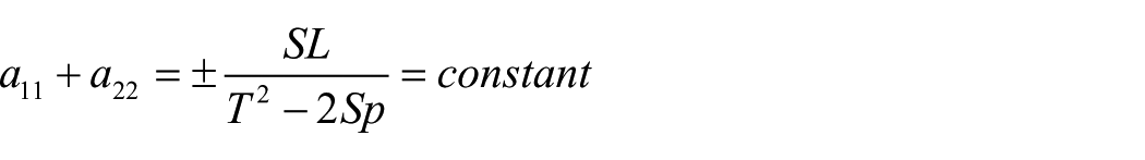
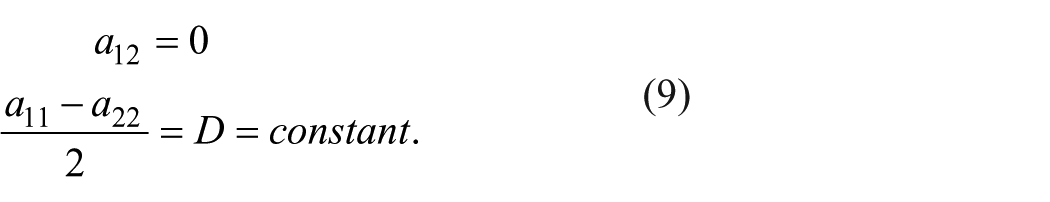
Alternatively, if we arrange the boundary conditions such that a11 = a22all around the boundary, then a11 – a22must be zero everywhere on the surface. and so
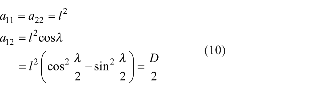
where λ is the angle between the two sets of springs of length l. D is the difference between the squares of the diagonals of a rhombus formed by the springs. Thus (9) and (10) are effectively the same case with the one set of coordinate curves being the diagonals of the other, and they correspond to exactly the same state of stress.
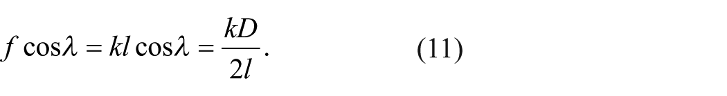
If k is the stiffness of the zero-length springs, then the tension in the springs is f = kl. The shear force on a node on a boundary parallel to the edge of the rhombi is
If we can arrange things such that that D = 0 in (9) or in (10), then we have a minimal surface on which the coordinate curves form curvilinear squares.
In Figure 13 the edge cable tension is kept constant, so that the zero-length springs are free to slide along the cables. Thus the zero-length springs meet the edge cable at 90, and therefore a12 = 0 on the boundaries so that a12 = 0 everywhere and in the case of Figure 13 D = 0 by symmetry, so that we have a minimal surface. The edge cables must be asymptotic lines on the surface to satisfy equilibrium of forces normal to the surface, and it follows that the zero-length springs follow the asymptotic directions.
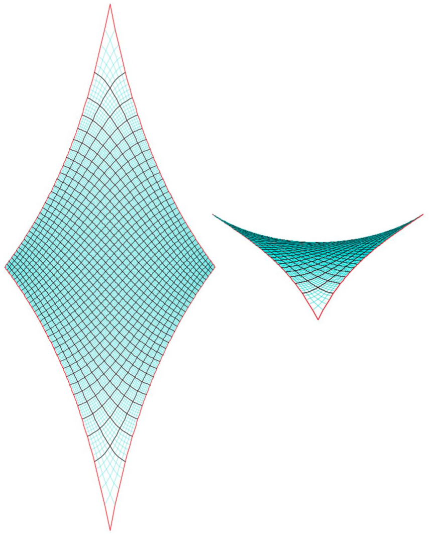
Minimal surface with asymptotic coordinates.
Figure 14 shows a surface with edge shear forces obeying (11), which means that we should find that we satisfy (10). Note that the spring lines will not be asymptotic directions.
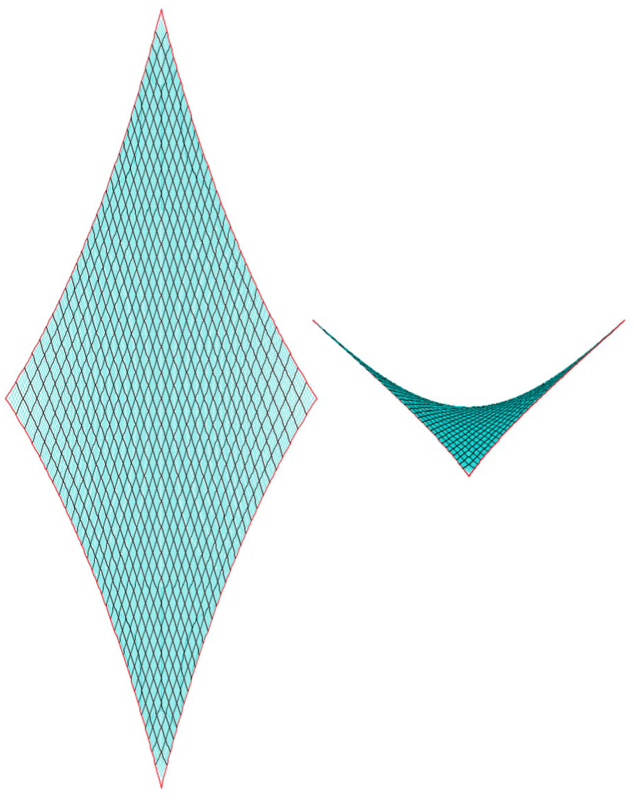
Surface with zero-length springs forming rhombi.
If we rotate the spring grid by 45 the springs follow the principal curvature directions as shown in Figure 15.
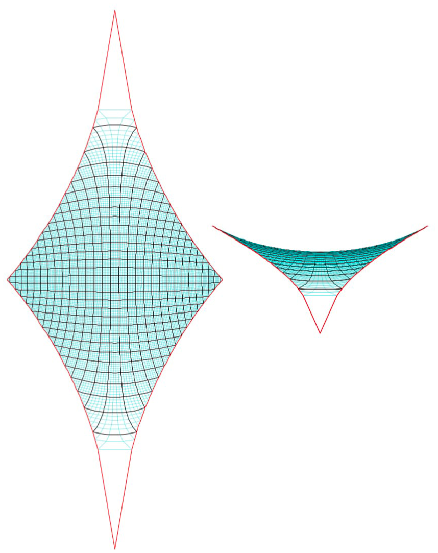
Minimal surface with principal curvature coordinates.
Figures 16 and 17 show more applications of geometries controlled by tension coefficients, which are constant in both figures.
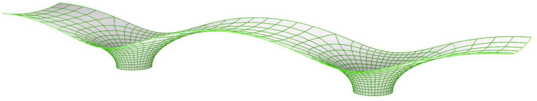
Minimal surface bridge, showing principal curvature lines, supported by a horizontal plane at the support, an inclined plane along the each long side and a vertical plane at each end.
Prestressed cable net.
If a minimal surface or soap film is bounded by a rigid surface, it slides sideways so that it is normal to the surfaces. If the bounding surface is a sphere or plane, then all directions are principal curvature directions with no twist. It follows from the Joachimsthal theorem 14 that the boundary curve on the minimal surface must be a principal curvature direction, unlike a cable boundary which is an asymptotic direction. This fact was used in automatically generating the principal curvature lines in Figure 16 simply by using the constant tension coefficients.
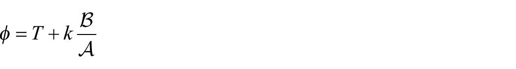
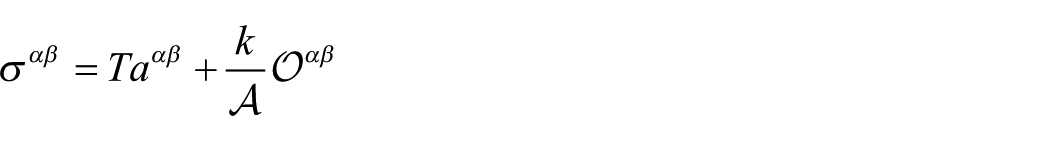
Zero-length springs plus a variable isotropic membrane stress
Now let us imagine that we have a membrane stress with components
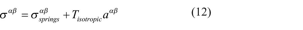
in which
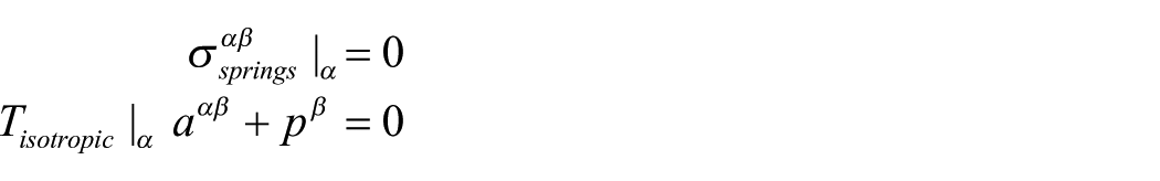
so that the tangential component of any load, particularly own weight is carried by
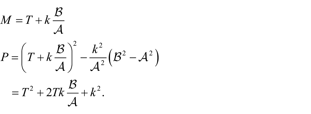
The mean membrane stress,
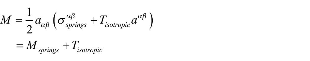
and the product of the principal stresses,
Thus (12) explicitly gives us both
Numerical strategy
The numerical models consist of nodes joined by linear and triangular elements
The linear elements exert forces on the nodes with components
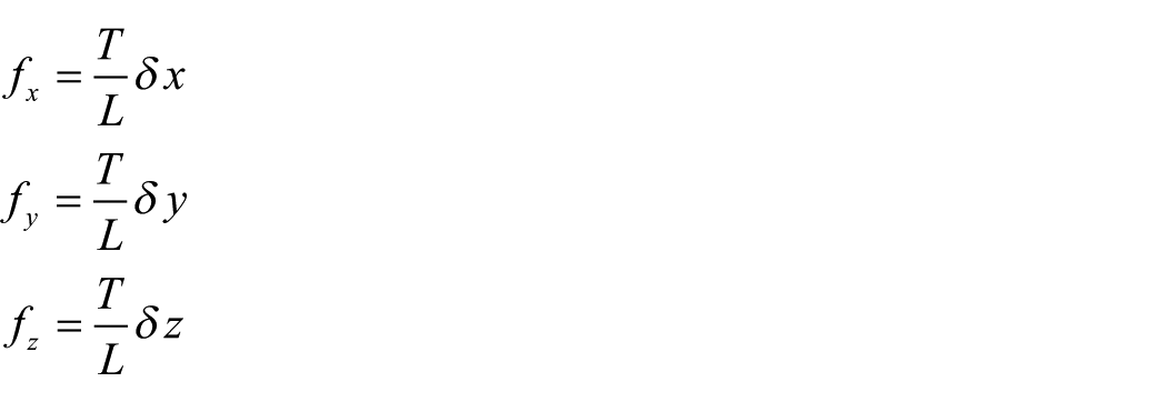
where
Triangular constant strain elements with three nodes are used to model an isotropic stress. The force on each node acts in a direction perpendicular to the opposite side and has magnitude equal to half the length of the opposite side times the isotropic stress. The triangular elements are also used to exert forces on the nodes due to the own weight of the surface and any pressure load on the surface, as in the bridge in Figure 9. The value of isotropic stress varies due to the tangential component of the own weight, as described in the section A soap film subject to its own weight above.
Having calculated the forces on each node, they are moved using Verlet integration, 17 which is the same as dynamic relaxation. 18 In fact we do not need to store the nodal forces since we can increment the velocities directly when we calculate the forces from each element.
It is relatively easy, but tedious, to program the above using the graphics processing unit (GPU). However our experience is that it is not worth using the GPU for this type of work, unlike, for example, three dimensional particle simulations.
Conclusions
In this paper we have described Weingarten surfaces in which the relationship between the mean and Gaussian curvatures produces a controlled spacing of the principal curvature trajectories.
We have also described a formfinding procedure which automatically generates a relationship between the mean and product of the principal membrane stresses. This in turn means that the spacing of the principal stress trajectories is controlled and not arbitrary. The numerical procedure of zero-length springs with a constant tension coefficient or force density plus isotropic soap film-like triangles in compression is relatively simple, although the theory is rather more challenging.
It should be noted that in general the principal curvature and principal membrane stress directions will differ, but in principal they could be made to coincide by adjusting the ‘cutting pattern’ of the zero-length spring net.
As stated in the introduction, it is ‘conventional’ in the design of shell structures to have a relatively ‘flimsy’ shell supported on ‘substantial’ edge beams, arches and cables. One of the aims of this work was to formfind shapes in which the forces that would have been concentrated in the edge beams or arches are distributed into the shell itself, more like the shells that we see in nature, 28 and it can be seen in the figures that the shells and tension structures have indeed been able to avoid edge beams, arches and cables.
In Appendix D we describe the theory of how a linear Weingarten surface can be obtained by the minimisation of a surface integral. We do not develop the practicalities of doing this and this could form the basis for further research.
Footnotes
Appendix A
Appendix B
Appendix C
Appendix D
Appendix E
Appendix F
Declaration of conflicting interests
The authors declared no potential conflicts of interest with respect to the research, authorship, and/or publication of this article.
Funding
The authors disclosed receipt of the following financial support for the research, authorship, and/or publication of this article: Emil Adiels gratefully acknowledges the funding received from Lars Erik Lundberg Scholarship Foundation (grant ID no. 1001904) and Åke och Greta Lissheds Stiftelse (grant ID no. 2025-029), both of which have provided essential support for his contributions to this research.