
Abstract
Fractional flow reserve is the current reference standard in the assessment of the functional impact of a stenosis in coronary heart disease. In this study, three models of artificial intelligence of varying degrees of complexity were compared to fractional flow reserve measurements. The three models are the multivariate polynomial regression, which is a statistical method used primarily for correlation; the feed-forward neural network; and the long short-term memory, which is a type of recurrent neural network that is suited to modelling sequences. The models were initially trained using a virtual patient database that was generated from a validated one-dimensional physics-based model. The feed-forward neural network performed the best for all test cases considered, which were a single vessel case from a virtual patient database, a multi-vessel network from a virtual patient database, and 25 clinically invasive fractional flow reserve measurements from real patients. The feed-forward neural network model achieved around 99% diagnostic accuracy in both tests involving virtual patients, and a respectable 72% diagnostic accuracy when compared to the invasive fractional flow reserve measurements. The multivariate polynomial regression model performed well in the single vessel case, but struggled on network cases as the variation of input features was much larger. The long short-term memory performed well for the single vessel cases, but tended to have a bias towards a positive fractional flow reserve prediction for the virtual multi-vessel case, and for the patient cases. Overall, the feed-forward neural network shows promise in successfully predicting fractional flow reserve in real patients, and could be a viable option if trained using a large enough data set of real patients.
Keywords
Introduction
Cardiovascular diseases (CVDs) are the world’s major cause of mortality, being responsible for approximately 31% of deaths worldwide. 1 Coronary heart disease (CHD) is the biggest sub-category of CVD, 2 and is most commonly caused by atherosclerosis build-up on the inner layer of a coronary artery, which narrows the vessel lumen area. The current gold standard diagnostic tool for estimating CHD severity is the fractional flow reserve (FFR), 3 although other diagnosis measures such as the instantaneous wave-free ratio (iFR) have been proposed.4,5 FFR is performed invasively during cardiac catheterisation. A pressure sensitive wire measures the pressure at the aorta and at a point distal to a stenosis simultaneously. The pressure ratio of pressure distal to stenosis divided by aortic pressure is used to determine if the stenosis is flow limiting. If the pressure decrease is greater than 20%, which corresponds with a FFR value below 0.8, the patient will normally be required to undergo further surgical treatment such as an angioplasty. As the FFR procedure is invasive and expensive, there have recently been attempts at determining the FFR non-invasively through the use of coronary computed tomography angiography (CCTA) and physics-based computational fluid dynamics (CFD) models.6–8 These models have been shown to give respectable agreement with the invasive clinical measures.
In recent years, there has been renewed interest in artificial intelligence (AI) with many areas now focusing on data science techniques to find correlations and predictions using data. This is partly due to two main developments: (1) the accessibility to much greater computational resources, and (2) the wider availability of large amounts of data that are required for training AI models. Some of these techniques are making significant inroads into medical research. Examples include AI algorithms being developed to detect cancer and determine a prognosis, 9 and to manage and support treatment of diabetes. 10 An AI model has even been shown to be more reliable at detecting brain tumours than the current techniques used in radiography. 11 Now, AI models are being applied to FFR, which ranges from replacing one-dimensional (1D) models with machine learning (ML) models, 12 to using the CCTA images and deep learning models to estimate the FFR directly from the CT images.13,14 While AI offers an excellent opportunity to compute FFR faster than the majority of physics-based models, assessing the accuracy and robustness remains a real challenge.
In the present work, we compare three ML models of varying degrees of complexity to further understand the applicability of AI in the FFR calculations. They are (1) multivariate polynomial regression (MPR), (2) feed-forward neural network (FFNN), and (3) a long short-term memory (LSTM) model. The ML models are first trained using a virtual patient database created using a validated 1D physics-based model, 15 then the ML models are compared with clinically invasive FFR measurements on a small cohort of 25 patients.
ML and deep learning
The foundation of current ML and deep learning algorithms originated from work in 1943 by McCulloch and Pitts. 16 . They proposed the idea and theory of a neuron, what it is and how it works, and created an electrical circuit of the model, thus creating the first neural network. In 1950, Turing 17 published the seminal paper ‘Computing Machinery and Intelligence’ that discussed the theoretical and philosophical ideas of AI. From this work, the Turing test was born. The normal interpretation of the Turing test is to have an interrogator attempting to distinguish between two ‘players’, one of which is human and the other is a computer. The development of ML and deep learning algorithms merely use the human nervous system, and in particular the brain, as a reference for inspiration in the development of these algorithms.
There has been a recent resurgence in the use of neural networks, primarily due to large amounts of data, and easier access to powerful computational resources. However, some of the fundamental mathematics used in AI are well established. For example, the gradient descent optimisation method, which forms the foundation of the back propagation step while training the model for many projects, was originally proposed by Cauchy 18 in 1847. Although at this stage gradient descent was used for minimisation problems on a system of simultaneous equations, it was not until the 1960s that gradient descent was used in the context of multi-stage, non-linear systems.19,20 In 1982, PJ Werbos 21 described the use of gradient descent in a neural network. The original gradient descent method is rarely used nowadays, but the improved optimisation methods of momentum 22 and ADAM, 23 essentially extend the gradient descent method and are widely used.
Methodology
Virtual patient generation and feature extraction from CT data
It is difficult to obtain a significant number of clinical patient data for training an ML model and hence we created virtual patients. There are two different types of virtual patient generation. The first considers a patient as a single vessel and randomises the vessel area profile, length, and flow rate through the vessel. These single vessel cases are used to train the ML models. The second case involves creating a network of the left coronary artery (LCA) branch that consists of nine main vessels.
Single vessel patient generation
The single vessel cases are generated by first randomising the proximal and distal area of the vessel independently in the range
The characteristics of the stenosis are also partially randomised. The stenosis is assumed to be located in the middle of the vessel. The severity of the stenosis is randomised between a
The stenosis is the constructed using the following equation
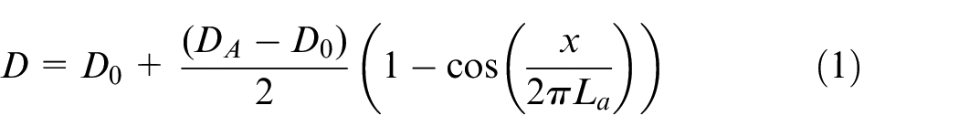
where
At this stage, the stenosed vessel undergoes an additional randomisation procedure to ensure that the vessel geometry is not too smooth. Across the length of the vessel, the first and last

where
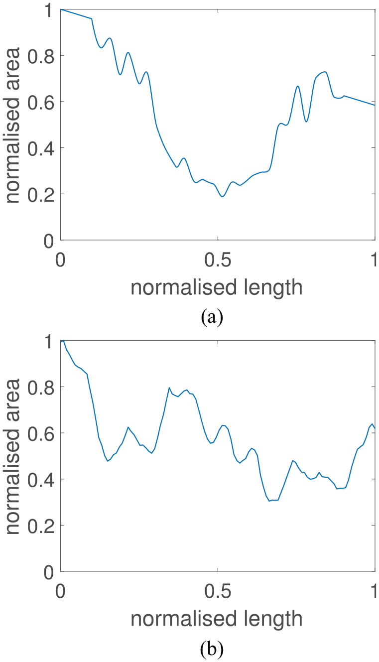
Normalised area profile of a generated patient and a normalised area profile of the left anterior descending artery extracted from a patient CT scan: (a) virtual patient area profile; (b) real patient area profile.
Virtual patient network generation
The virtual patient network uses the left coronary network branch consisting of nine vessels, presented in Mynard and Smolich,
24
as the foundation for which vessel area and length adaptations are performed. On top of this foundation, a similar randomisation procedure is performed to that of the single vessel case. First, in the procedure is that the length, and the area at the start and end of every vessel are all randomly adapted by increasing or decreasing around their reference state by up to
Feature extraction from CT images
In order to extract the features from the patient CT images, the images first need to be segmented. The segmentation and extraction of centreline information is performed using the image segmentation software VMTKLab (Orobix, Italy). The area profile and vessel length information can then be extracted and can be used to find the input features for two of the ML models, which include the area at the start and end of each vessel, the mean vessel area, and the vessel length. The volumetric flow rate at the inlet of the LCA is assumed to be
ML
Many of the concepts and theory used in ML were previously developed in other areas of mathematical sciences, such as using statistics to find the likelihood of an event occurring or finding relationships and correlations in various types of data. One such method is MPR, which is a generalised form of linear regression.
MPR
MPR is the least complex model implemented in this work and utilises linear regression with a high-order polynomial feature space on multiple variables. Although polynomial regression is quite simple, it can still provide useful and powerful predictions. However, one must be careful when creating the training and test data for these models as polynomial regression tends to perform reliably well when used to interpolate data, but can produce erroneous predictions when attempting to extrapolate data. This issue is often exacerbated when higher-order polynomials are used for the feature space. In order to describe this method, it is advantageous to first describe univariate polynomial regression, and then discuss its extension to the multivariate case.
Univariate polynomial regression for a dependant variable

where
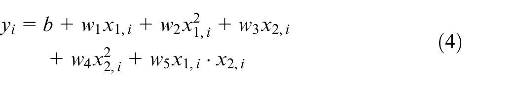
which contains the multiplication of the two independent variables to create the new feature

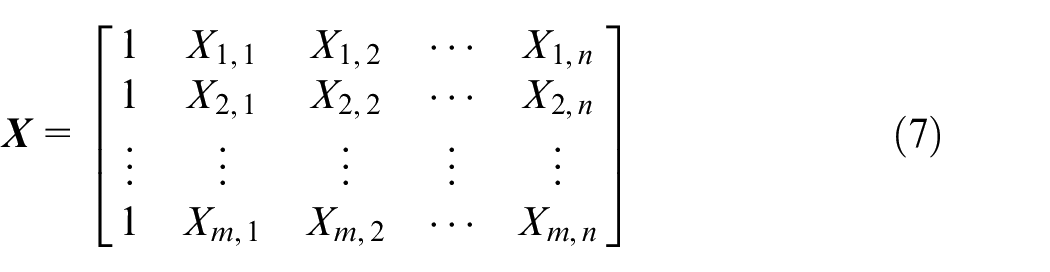
where

containing all outputs/predictions, where
where

In the present article, the least-squares method is used to solve for the bias and weight terms for polynomial regression. Six input features are used which includes the area at the start and end of a vessel, the minimum area in the vessel, the mean area of the vessel, the estimated flow rate in the vessel, and the length of the vessel.
Deep learning
In biomedical engineering, the more basic statistical techniques such as polynomial regression have generally fallen out of favour. These have largely been replaced by artificial neural networks (ANNs), which are considered as more powerful alternatives when it comes to finding correlations in complex real-world data. The term ANN was used as they are inspired by, and try to resemble the human nervous system, and particularly the human brain. The human brain is composed of many interconnected neurons which transmit information in the form of electrical impulses. Analogously, ANNs are composed of layers of interconnected ‘neurons’ which pass information to and from other neurons.
The ‘depth’ of a neural network generally refers to the number of hidden layers that are present in an ANN, and in general increasing the number layers in an ANN allows a greater degree of non-linear features to be captured. There are many types of deep learning architectures, each with different strengths and weaknesses. In addition, there are three main paradigms of deep learning which are supervised learning algorithms, which seek to find a relationship between input features of training data to their known outputs; unsupervised deep learning algorithms, which seek to find patterns in data without knowing any result or outputs; and reinforcement learning, which is a goal-oriented algorithm that seeks to learn the best possible action to maximise its ‘rewards’ for a particular situation, and thus learns from its experience.
The two types of supervised deep learning models utilised in the present article are an FFNN, and an LSTM model which is a type of recurrent neural network (RNN).
Non-linear activation functions
The activation functions utilised in this article (including those used in the LSTM) are shown in Figure 2 and are the rectified linear unit (relu) function which is given by

and is most often used for regression problems, has an output range of [
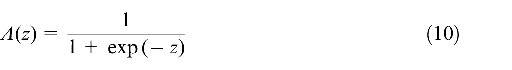
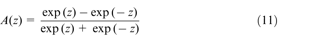
The logistic function is more often used in classification problems; the final activation function used in this article is tanh which also tends to be used in classification problems, has an output in the range [
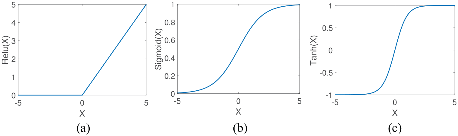
Comparison of the most common non-linear activation functions for FFNN networks: (a) relu activation function; (b) logistic (sigmoid) activation function; and (c) tanh activation function.
FFNN
FFNNs consist of an input layer, and output layer, and at least one hidden layer. FFNN is a supervised learning technique that utilises non-linear activation functions at each layer (with the exception of the input layer), in order to capture non-linear relationships in the data. FFNNs are referred to as vanilla neural networks when they have only one hidden layer. A diagram of a FFNN network is shown in Figure 3, where each arrow shown in the diagram represents a linear mapping, followed by a non-linear activation function as indicated in Figure 4. Training an FFNN typically involves four main steps (steps are expanded upon in the next three paragraphs): (1) forward propagation which computes the predicted output value from an initial estimation of weights and biases. The direction of computation is from the input layer through to the output layer (hence it travels forward); (2) computing the cost function (error) of the predicted output to the expected output; (3) backward propagation which computes the derivatives of the cost function with respect to the weights and biases. The direction of computation is from the output layer through towards the input layer (hence it travels backward); (4) finally, the derivatives that were calculated from backward propagation are used to update the bias and weight values.
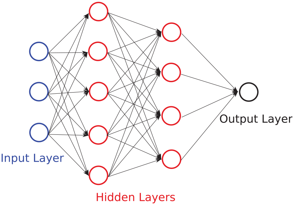
Example of a FFNN with an input layer of three features, two hidden layers of five and four neurons, respectively, and an output layer with a single neuron. Bias terms are neglected in this diagram to reduce complexity.
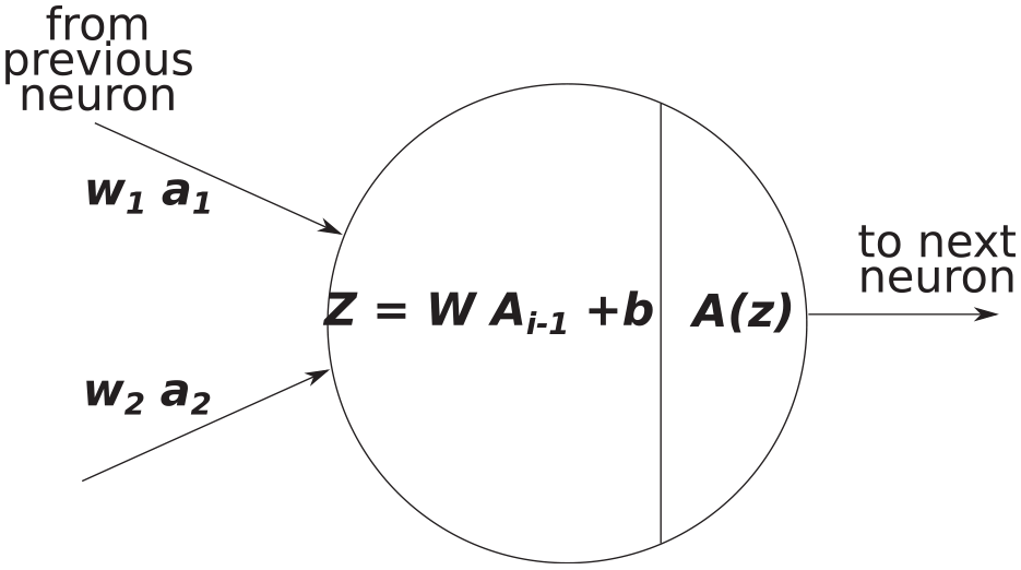
Example of an input and output of a single neuron during forward propagation, where
FFNN training
The FFNN training process begins with the initialisation stage which includes randomising the weights and biases, and giving the algorithm the training set of input features. The next step is forward propagation which involves a linear mapping for outputs from neurons in the previous layer to neurons in the next layer as

where
The general initialisation and forward propagation algorithm for the FFNN utilised in the present work is as follows:
define input features and select the training set,
initialise weights and biases for each layer,
linear mapping from input features to hidden layer 1,
non-linear activation function (relu),
linear mapping from hidden layer 1 to hidden layer 2,
non-linear activation function (tanh),
linear mapping from hidden layer 2 to hidden layer 3,
non-linear activation function (relu),
linear mapping from hidden layer 3 to the output layer,
non-linear activation function (relu) for FFR prediction.
After the forward propagation is complete, a cost function is used to calculate the error in the prediction compared to the actual values. The most common type of cost function for regression problems is the mean square error
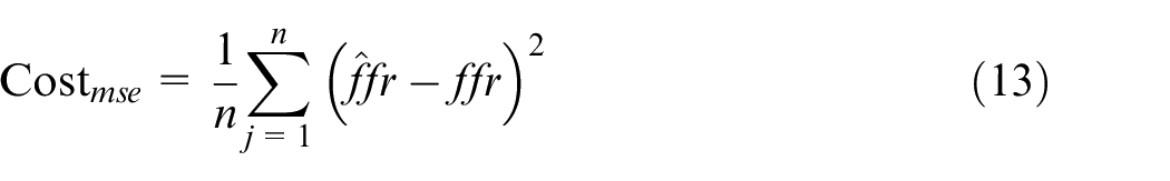
where
The next step is to perform backward propagation, the first part requires the calculation of the derivative of the cost function with respect to the predicted values
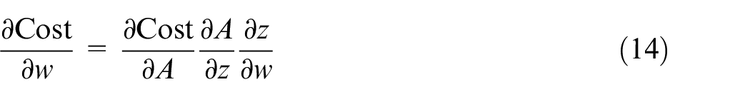
The general implementation of the backward propagation algorithm for the FFNN is as follows:
calculate the derivatives of the cost function w.r.t. the weights and biases for the output layer,
calculate the derivatives of the cost function w.r.t. the weights and biases for hidden layer 3,
calculate the derivatives of the cost function w.r.t. the weights and biases for hidden layer 2,
calculate the derivatives of the cost function w.r.t. the weights and biases for hidden layer 1.
The weights and biases can then be updated for all layers via an optimisation algorithm such as gradient descent or ADAMs optimisation. For the FFNN model, the ADAMs optimisation 23 was used to find a local minima.
In order to predict FFR values from new input features, forward propagation can be performed with the final converged weights and biases.
FFNN model description
The FFNN model implemented in the present article uses an input layer of six features that includes the area at the start and end of the vessel, the minimum area in a vessel, the mean area of a vessel, the estimated flow rate in the vessel, and the length of the vessel. There are three hidden layers, the first hidden layer contains 64 neurons and uses the relu function, the second hidden layer contains 32 neurons and uses the tanh function, and the third hidden layer also uses 32 neurons but uses the relu function; the output layer gives a single FFR output value for the end of the vessel and uses the relu function. The architecture was chosen from iteratively trialling different combinations of the number of neurons in a layer, the number of layers, and the type of activation function used, all using grid searching. It is known that for many problems the relu function increases the speed of convergence; however, it was observed that model training performed better with at least one layer of the tanh function. The model did not require any additional techniques to prevent over-fitting to the data as the training and test accuracy were both close to 99%. The ADAMs optimisation algorithm is used to update the model weights and biases. The learning rate used was
LSTM
In the medical arena, there are many diagnostic and monitoring systems that take time dependant measurements and can be viewed as sequence data. RNNs are particularly convenient for these problems as they can exhibit dynamic temporal behaviour and can have sequence data as a model input and as an output. An RNN cell contains a closed-loop which allows the output of the current step to be influenced by the output of the previous step. In theory, RNNs are able to use previous values in the sequence to aid in predicting a future value (time dependencies) and they tend to perform quite well when the distance between a point and a dependent value is quite small; however, in practice, they often struggle with longer-term dependencies.25,26 This shortcoming was resolved with the development of the LSTM algorithm.
27
LSTMs have a different structure for a module, which instead of having a single layer that contains a loop, the module now contains four structured layers with a loop, although several LSTM variations exist. Fundamental to the structure of an LSTM model is the idea of gates, which includes an input gate, a forget gate, and an output gate. An important characteristic of LSTM is in its ability to add or remove information from the sequential inputs given to it, which allows it to retain useful information and remove inessential parts automatically. Each LSTM ‘cell’ contains two states in parallel, an internal cell state
initialise weights, biases, cell states, and output states,
forget gate has inputs

3. input gate and cell state update
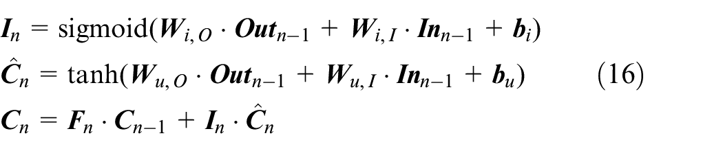
4. output gate and output vector
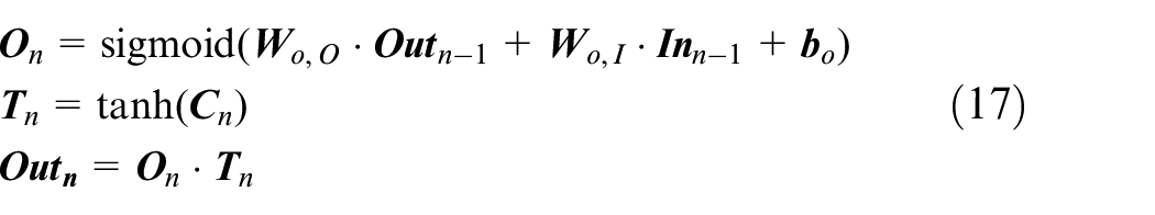
The output state and cell state at step
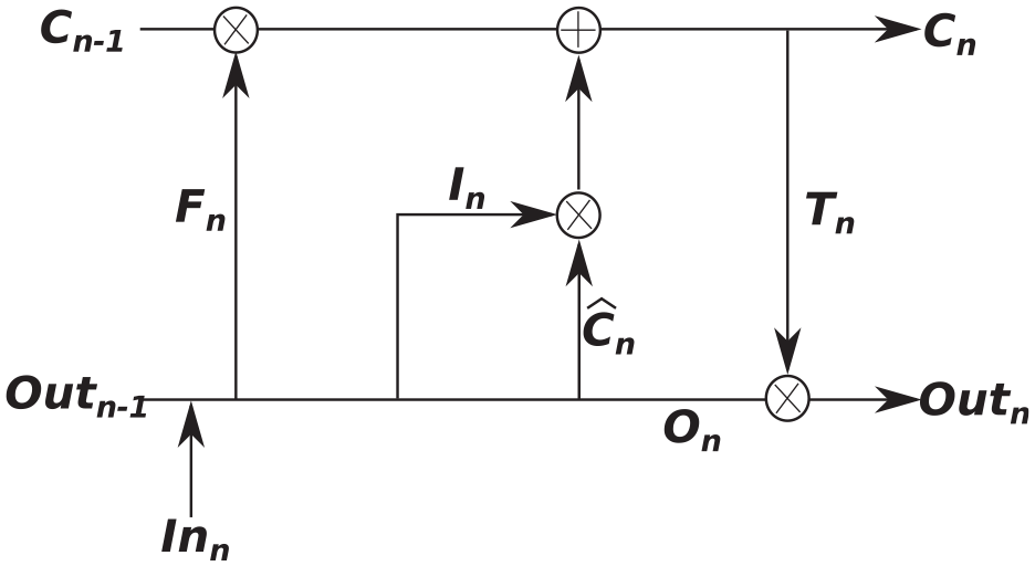
Overview of an LSTM module.
In this article, the stacked LSTM model is made up of five LSTM layers all with 32 modules, followed by five fully connected (dense) layers with 32, 32, 16, 8, and 1 neurons, respectively. The learning rate used was
Computational mechanics
One of the main limitations that can hinder ML and deep learning model development is the ability to collect an adequate amount of real-world data for training the model. This is particularly the case in biomedical engineering where there are many issues that impact the ability to collect real patient data, such as the number of patients that have a particular health problem, the type of data that is collected in the medical clinic may not be exactly what is needed to correctly model the problem, some data may be missing (some patients may not have pressures recorded while others do), and the quality of the data itself is affected by the accuracy of the measurement device or the quality of the imaging data. Thus, in the present article, we utilise a 1D haemodynamic model that has been previously validated against invasive FFR measurements8,15 in order to generate virtual FFR patients. These virtual patients are then used to train the three AI models.
The 1D model of blood flow utilised in the present article is described in Carson and colleagues15,28 and contains two tiers: (1) the closed-loop model that is described in Carson and colleagues28,29 is used to generate the flow rate waveforms for the inlet of the left coronary and right coronary arteries; (2) an open-loop coronary network (the coronary network in Mynard and colleagues24,30) is then used, where the vessel length and areas are adapted at random to produce similar vessel area variations to what is seen in real patient data, in addition a stenosis is added to one of the vessels in the network using a random blockage percentage, stenosis length, and stenosis location.
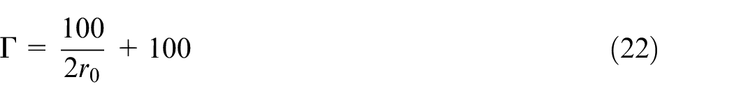
The 1D model of blood flow in a compliant vessel is governed by the continuity equation
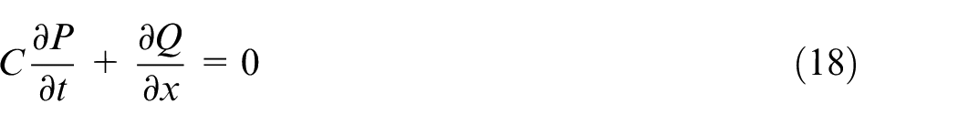
where
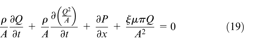
where
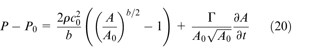
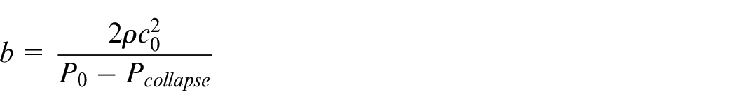
where
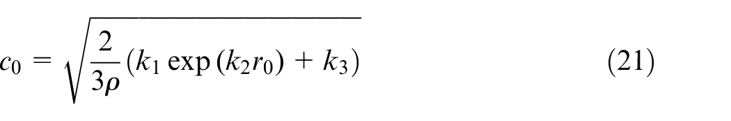
where
To be consistent with the ML models, conservation of static pressure is assumed at the junction of vessels. The system of non-linear equations is solved using an implicit sub-domain collocation scheme. 31
Constructing an ML model of FFR on a coronary network
In the present work, two separate model constructions are proposed, respectively, using the pressure drop and the FFR value. The MPR and FFNN are trained using a single vessel model for the pressure drop (rather than FFR value), and the RNN (long-short term memory) model is trained on a single vessel model for the FFR value. This is performed for the following two reasons:
There are large variations in patient coronary network geometry that includes different vessel sizes (lengths and areas), different vessel connectivities, and the inclusion or exclusion of certain vessels. The MPR and FFNN models only use six input features; thus, all variations in patient geometry need to be covered by these six features. Through tests on the 1D model, 15 the pressure drop across the stenosis is invariant to the aortic pressure, while the FFR value intimately depends on the aortic pressure. This means that the pressure drop is more reliable and easier to utilise for training these models, as the number of input features is low.
the LSTM model is ideal for sequences and thus it is a natural choice for a network in which the solution in the next vessel will depend on the solution of the previous vessel. However, as all input sequences (vectors) must have the same length, post sequence zero-padding is performed for the area profile.
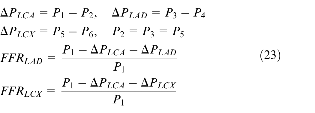
In order to describe the construction of the FFR solution in a network for the MPR and FFNN models, we first make the assumption (validated through numerical tests) that the pressure drop in a vessel is not influenced by the hydrostatic pressure at the start of the vessel. Second, we assume continuity of static pressure at vessel junctions (although an ML model could also be used to estimate the change in pressure between vessels). These two assumptions allow the use of a simple reconstruction technique to determine the FFR value from the aorta to the location of FFR measurements downstream of a stenosis. Thus, the MPR and FFNN models estimate the pressure drop over each vessel in a network which is reconstructed in the following way: consider a bifurcation of the LCA, left anterior descending (LAD) artery, and left circumflex (LCX) artery as shown in Figure 6.
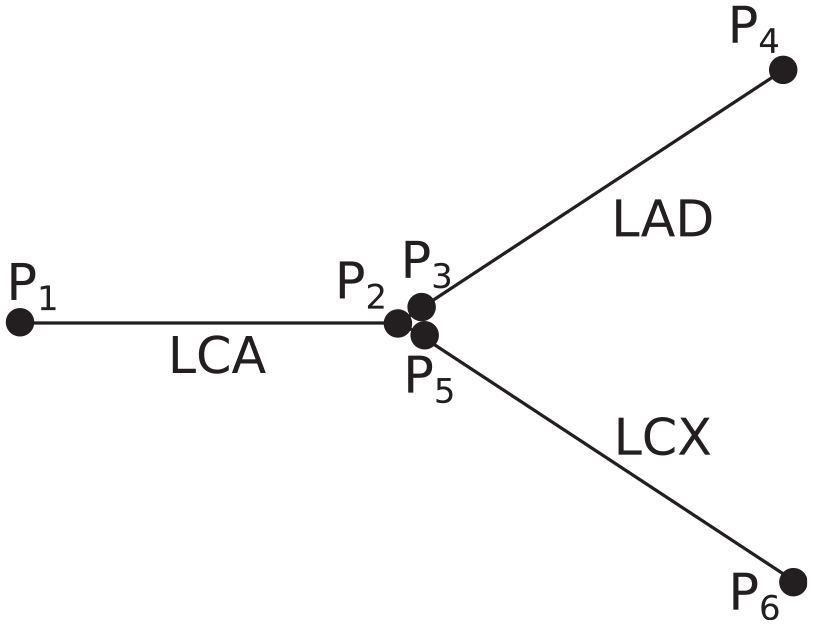
Three-vessel configuration consisting of an LCA, LAD, and LCX. For the MPR and FFNN models, the pressure drop is calculated across each vessel separately and then the FFR values are reconstructed afterwards.
There are six pressure ‘nodes’ representing the pressure at the start and end of the three vessels. For continuity of static pressure at vessel junctions, the pressure at the end of the LCA will be equal to the pressure at the start of both the LAD and LCX vessels. Thus, the FFR value at the end of the LAD and LCX can be reconstructed from the pressure drops (
This technique can be extended in a straightforward way to any size of vessel network, provided a good estimation of the mean aortic pressure is known. In the present work, we estimate that the mean aortic pressure is
Results
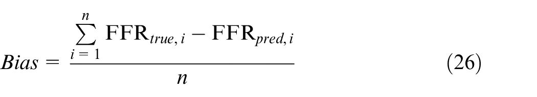
In order to test and compare the proposed methodologies, three test cases are constructed. The first test case uses a virtual patient database of single vessels. In reality, the FFR measurement does not take place at points just either side of the stenosis, but instead the proximal pressure measurement occurs in the aorta near where the coronary arteries branch out from, while the measurement point distal occurs after a stenosis; thus, the full FFR ratio is affected by what happens over a vessel network and not over a single vessel. Thus, we test our reconstruction methodology on the second test case, which consists of a network of virtual patients where the FFR solution is determined by the 1D CFD model, and in the third test we evaluate the methodology on a small cohort of real patients where the FFR has been measured invasively during coronary catheterisation. In our results, the mean absolute error (MAE) that is calculated as
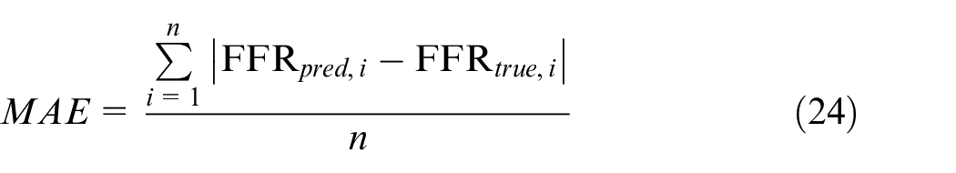
where
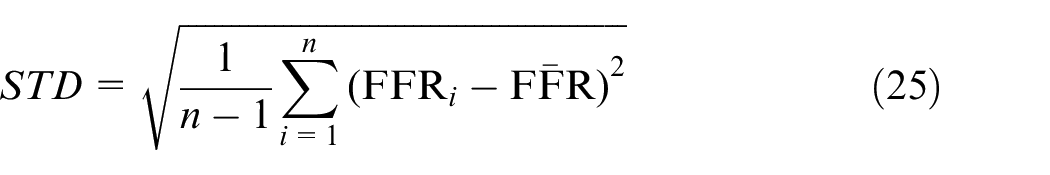
where FFR is either from the ML predicted models, CFD model, or invasive FFR measurements, respectively, and
Results from single vessel
The first test case uses a virtual patient database of single vessels using the 1D blood flow model where the virtual patients were created by randomising the vessel area profile, stenosis location, stenosis length, stenosis severity, and the mean inflow rate. A total of 10,000 single vessel ‘virtual patients’ were generated with 70% used for model training and 30% used for testing. Figure 7 shows the results of the test set for all proposed methodologies, and Table 1 shows the overall performance of each methodology. The diagnostic accuracy is consistent between all of the models where they all achieve just under 99% accuracy. The sensitivity and specificity are closer in value for the MPR. For the FFNN model, the specificity is higher than the sensitivity, while for the LSTM model this is exacerbated further with the sensitivity 95.76% while the specificity is 100%. All methodologies show a very high linear correlation value and p-value of 0. Although the results are very consistent between the three models, the FFNN performs the best on this test case as it has the equal highest diagnostic accuracy with the lowest MAE when compared to the 1D physics-based model. The standard deviation of the test set used in this example was
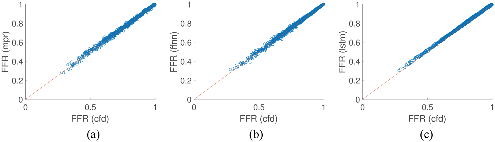
Comparison of machine learning/deep learning methods against the CFD model results on a single vessel: (a) MPR results on test set; (b) FFNN results on test set; and (c) LSTM results on test set.
Overview of the test set for each machine learning model compared to the 1D physics-based model on a single vessel model.
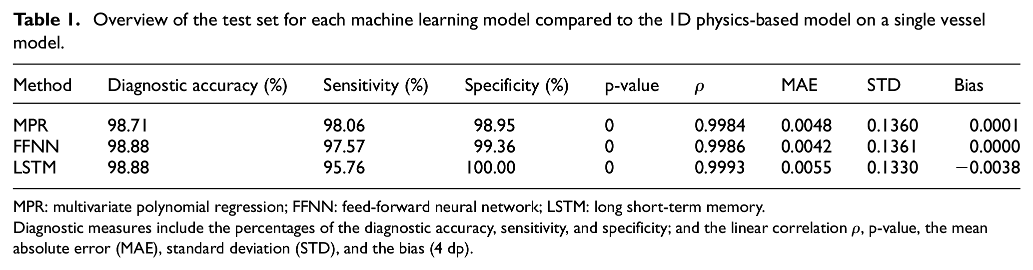
MPR: multivariate polynomial regression; FFNN: feed-forward neural network; LSTM: long short-term memory.
Diagnostic measures include the percentages of the diagnostic accuracy, sensitivity, and specificity; and the linear correlation
Multi-vessel FFR
The second test case utilises a virtual patient database of LCA vessel networks. The left side of the coronary network proposed by Mynard and Smolich
24
is used as a basis, while the area profiles, vessel lengths, stenosis location, length, and severity, and flow rate distribution are varied randomly. A cohort of 10,000 virtual patient coronary artery networks were generated, each network contained nine vessels, with 70% used for model training and 30% used for testing for all ML models. As shown in Table 2 and Figure 8, the FFNN model performs the best with a diagnostic accuracy of over 99% and also had the lowest mean absolute difference and highest linear correlation value. The LSTM, which is the most complex model implemented in this work, had the lowest diagnostic accuracy; however, it still had a lower mean absolute difference from the 1D physics-based model than the MPR model. The standard deviation of the underlying data in synthetic multi-vessel case was
Comparison of the MPR, FFNN, LSTM models with the 1D physics-based model on a nine-vessel network.
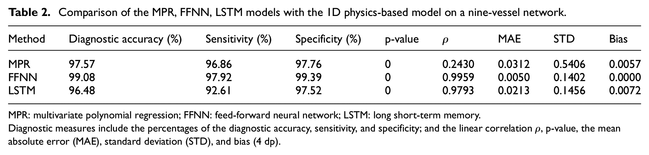
MPR: multivariate polynomial regression; FFNN: feed-forward neural network; LSTM: long short-term memory.
Diagnostic measures include the percentages of the diagnostic accuracy, sensitivity, and specificity; and the linear correlation
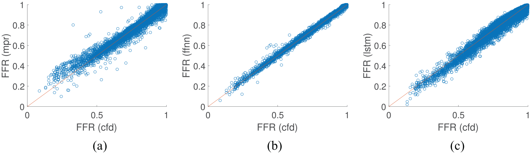
Comparison of machine learning/deep learning methods against the CFD model results on coronary artery vessel networks: (a). MPR results on test set; (b) FFNN results on test set; and (c) LSTM results on test set.
Comparison with invasive FFR
The final test case compares the proposed methodologies and the 1D physics-based model to clinical invasive FFR measurements that were performed under coronary angiography for a cohort of 25 patients.
15
The results are shown in Figure 9. It is important to highlight that although 25 FFR values are compared, only 23 cases had the exact FFR value from the clinic. For two of the cases, the FFR was only recorded as positive (FFR < 0.8) or negative (FFR ≥ 0.8), respectively. These two cases are shown in Figure 9 as
Comparison of the MPR, FFNN, LSTM, and 1D physics-based model with invasive clinical measurements in the patient-specific networks.
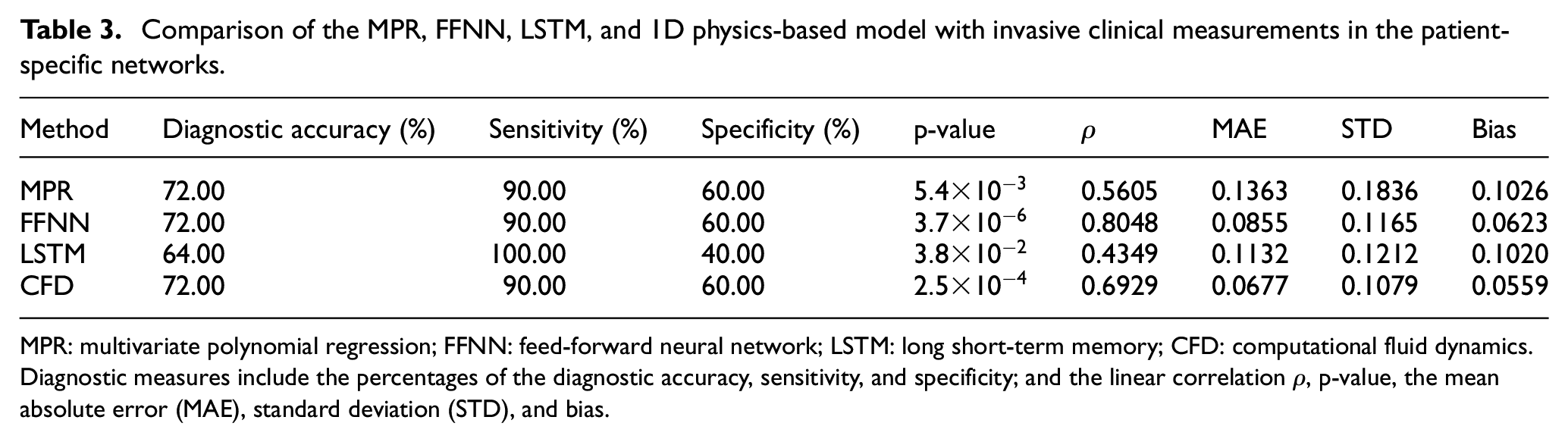
MPR: multivariate polynomial regression; FFNN: feed-forward neural network; LSTM: long short-term memory; CFD: computational fluid dynamics.
Diagnostic measures include the percentages of the diagnostic accuracy, sensitivity, and specificity; and the linear correlation
Comparison of the MPR, FFNN, LSTM, with the 1D physics-based model.
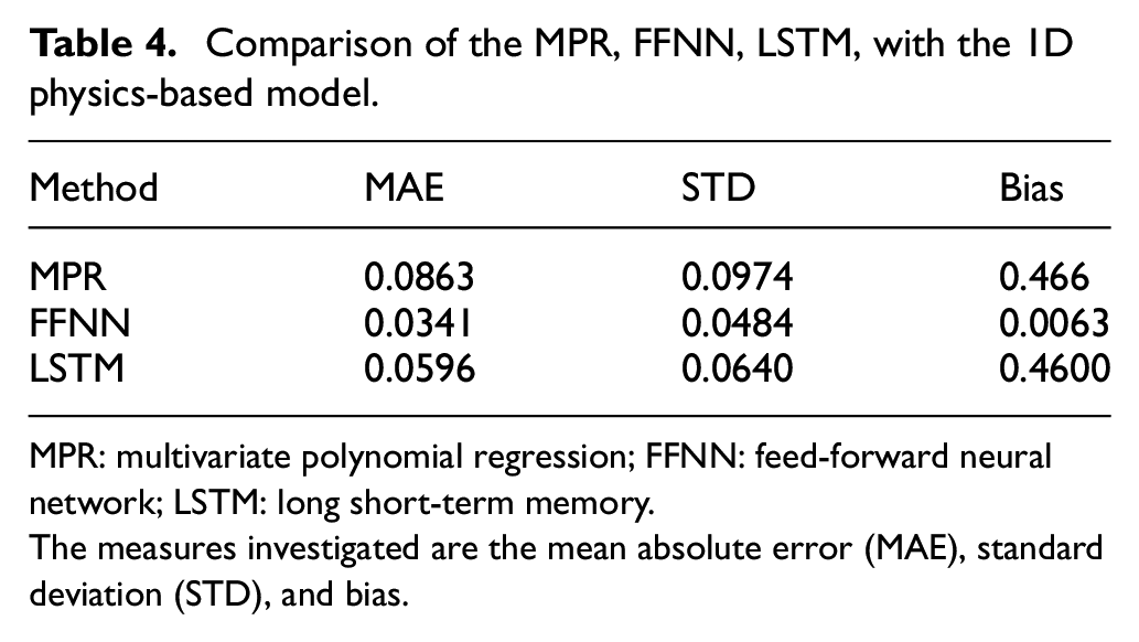
MPR: multivariate polynomial regression; FFNN: feed-forward neural network; LSTM: long short-term memory.
The measures investigated are the mean absolute error (MAE), standard deviation (STD), and bias.
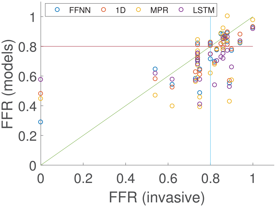
Comparison of the 1D physics-based model and the three machine learning/deep learning methods against the invasive clinical measurements on the coronary artery vessel network of 25 patients.
Discussion
For the single vessel case in Figure 7, the LSTM showed the least spread of FFR prediction and highest linear correlation, although there is no significant difference between the diagnostic performance of the methods employed. Generally, the LSTM model showed bias towards the specificity implying that it is biased towards a positive FFR prediction (FFR > 0.8). Interestingly, the LSTM method gave the largest MAE which is mainly due to the bias as discussed above. All three of the ML-based methods were shown to give respectable FFR predictions when compared to the 1D physics-based model on single vessels, although the FFNN was shown to have the lowest MAE. However, in the clinic, the FFR measurement takes place between the aortic pressure to a point distal to a stenosis, and therefore it is very rare for only a single vessel to be considered.
In the multi-vessel case in Figure 8, there is a more noticeable difference in the quality of the results between the methods. This case is more challenging than the single vessel case as there is significantly more variation in the flow rates, vessel lengths, and area profiles. The MPR struggles to account for this variation. The training set and test set come from the same distribution of input features as required to create a well-defined ML model. However, some of the test set contained input feature variations that were not observed in the training set and thus the models needed to extrapolate the data to give predictions. As a result, the MPR model has the largest MAE and by far the lowest linear correlation value. MPR gives several erroneous predictions (not seen in Figure 9 as these values are extreme), for example, the maximum FFR predicted by the MPR is
When comparing the ML models and the 1D physics-based model from which they were originally trained with the invasive clinical measurements, the FFNN again shows the best predictive power of the AI models. Again, the MPR has the highest MAE; however, the diagnostic accuracy, sensitivity, and specificity are the same for the FFNN, MPR, and 1D model. The LSTM performs worse than the other methods in terms of diagnostic accuracy, and is generally biased to predict a positive FFR. This may be due to the LSTM using zero-padding, which although required, can influence the accuracy of the model, 35 and there is more network variation in the patient data compared with the training cases (patient cases range from 3 vessel networks to 12 vessels in the network). The LSTM model is the most complex of the two deep learning approaches and may have been expected to outperform the FFNN model. However, the input for the LSTM model is the entire area profile of each vessel in the coronary network, while the FFNN only considers six input features as it is not considered effective at handling sequence data. This essentially means that the LSTM had to learn more complex relationships. In addition, gives a more informative output prediction for other regions in the coronary vessel as the output of the LSTM is the FFR values across the entire length of the network, while the FFNN model only gives a single FFR value at the end of a vessel.
It is observed that the standard deviation of the synthetic data is significantly higher than that in the real patient data. Due to the small patient cohort in this work, and that the majority of the cohort had an FFR measurement in the range 0.75–0.9, the standard deviation of the real patient cohort was relatively small. In order to successfully train an ML model that can generalise to predict FFR, it was deemed necessary to have a greater spread, and thus larger standard deviation, in the synthetic patient cases. This lowers the likelihood of over-fitting the ML models, and can help generalise it for any future patient cases tested that are outside the range observed in the current real patient cohort utilised in this study.
Although ML models can effectively be used to replace aspects of physics-based models, there are several aspects that need to be addressed before AI can be used in medicine for direct diagnostic and treatment decision-making. There have been several AI-based models for FFR that have been proposed, ranging from replacing the physics-based models, 12 predicting FFR from the segmented vessels, 36 to making the prediction directly via the CT scans.13,14 However, utilisation of these AI predictions in the clinic raises ethical and validity issues, which still need to be appropriately addressed. 37 Another issue involved in non-invasive FFR is the extraction of the coronary geometry from the CT data. This is a particular stumbling block for both physics-based models and ML techniques. However, deep learning techniques and computer vision can be effective at identifying objects in images. It is not beyond the power of a deep learning algorithm to be used to extract the required coronary vessel features directly from the CT images. Although this would also require a significant number of CT images to train any model.
Although AI models could be utilised to replace the well-established physics-based models in areas such as medical research, there is an argument that AI could supplement existing physics-based modelling, and rather be focused on replacing or improving the bottlenecks in this area of medical research, which is segmentation of the CT scans. This is in part due to the fact that that the well-established reduced-order models are already very fast, and have been shown to give good accuracy; while segmentation is the slowest part of the non-invasive FFR prediction process, 15 and is often the most variable aspect of the prediction process with significant differences in segmented geometry observed between experienced users, 38 and even between different CT scanners. 39 AI could be used to reduce the amount of segmentation required, or even replace it entirely, which has been achieved for good quality CT images. 40
Limitations
In this work, only a small cohort of real patient measurements was suitable for FFR prediction using ML. This needs to be increased significantly in order to train the ML models using real patient data, rather than on a validated 1D physics-based model that is used as a surrogate.
Conclusion
In this study, three AI models of varying degrees of complexity were compared to invasive FFR measurements. The AI models were initially trained using a 1D physics-based model on a virtual patient database. The AI models, in order of least complex to most complex, are the MPR, the FFNN, and the LSTM model. The models were compared to single vessel, and multi-vessel network cases from the virtual patient database, and also on clinically invasive FFR measurements. The least complex model, the MPR, struggled with the significant variation of area profiles, lengths, and flow rate estimations in the data, and produced some erroneous predictions. The most complex model, the LSTM performed well for the single vessel cases, but did not perform as well for the multi-vessel network and patient cases. The FFNN performed well for all cases.
Footnotes
Acknowledgements
The authors gratefully acknowledge the contribution of Prof. Carl Roobottom and Dr Robin Alcock in supplying the anonymised patient data from Derriford Hospital and Peninsula Medical School, Plymouth Hospitals NHS Trust, used in this work.
Declaration of conflicting interests
The author(s) declared no potential conflicts of interest with respect to the research, authorship, and/or publication of this article.
Funding
The author(s) disclosed receipt of the following financial support for the research, authorship, and/or publication of this article: This work was supported by Health Data Research UK (MR/S004076/1), which is funded by the UK Medical Research Council, Engineering and Physical Sciences Research Council, Economic and Social Research Council, Department of Health and Social Care (England), Chief Scientist Office of the Scottish Government Health and Social Care Directorates, Health and Social Care Research and Development Division (Welsh Government), Public Health Agency (Northern Ireland), British Heart Foundation and the Wellcome Trust.