Cycle model matching of a regional aircraft engine using high-fidelity flight simulator data

Abstract

A thermodynamic cycle model was matched to the CF34-8C5B1 engine using the data of a high-fidelity Level-D flight simulator as a surrogate. Before the model match, the data from the simulator was assessed to determine thermal stability, data reproducibility, and engine-to-engine variation. A series of tests were performed across the flight envelope of the MHI CRJ-700 regional aircraft to match and validate the intended cycle model. A baseline off-design cycle model was established based on an engine design point from previous research. This baseline model allowed the detection of any suspicious data obtained from the flight simulator and made it possible to determine appropriate actions concerning the model match. The baseline thermodynamic model was then adjusted and calibrated to match the data from the simulator at various flight conditions. The cycle model adjustments involved: (1) recalibration of the speed lines of the fan map, and (2) tuning the low-pressure turbine map’s adiabatic efficiency. These variables were selected based on the physics of the problem. Moreover, a simplified matching method was proposed, which allows to optimize the processing time and circumvent convergence problems. The proposed adjustments render a final model that predicts the thrust and engine fuel flow rate of the CF34-8C5B1 engine within ±5.0% relative to the flight simulator engine model for the power settings of interest.

Introduction

Currently, turbofan Gas Turbine Engines (GTEs) power the majority of the commercial aircraft fleet. According to Airbus Inc., ¹ the installed fleet (corresponding to aircraft ≥100 passenger and freight above 10 tonnes) was about 22,680 aircraft at the beginning of 2019, and it is expected to reach 47,680 by 2038; roughly doubling in the next 20 years. Indeed, this growth forecast was elaborated before the global pandemic of Covid-19, which significantly impacted transportation in general due to travel restrictions and lockdowns. However, in Ref. 1 it is remarked that a two-fold growth (approximately) has been observed every 20 years in spite of health or financial world crises (e.g., SARS, oil crises, etc.). With the projected growth forecast for the aviation industry, one challenge is to achieve the fleet growth while meeting the envisioned 2050 carbon emissions neutrality target. ²

Significant efforts are being undertaken across the industry (aircraft and engine manufacturers, governments, regulatory agencies, researchers, etc.) to reduce the dependency on carbon-based fuels and/or mitigate their harmful effects. Novel technologies are getting significant attention (e.g., hybrid electric ³ and fuel cells ⁴ ) for alternative means of propulsion; however, at the present time, they are not sufficiently matured for replacing GTE. Even the ambitious forecasts predict some of these technologies to entry into service only by 2035/40. ⁵ Hence, the industry is heavily reliant upon keeping GTEs while transitioning to sustainable aviation fuels, ⁶ which are forecasted to contribute to about 60% of the emission reduction for the 2050 target. ⁵ Another potential alternative is the introduction of Liquid Hydrogen (LH2) fuel.^7,8 While using LH2 fuel in aircraft applications has been studied since the 1950s, ⁹ it is still a challenge today. LH2 fuel cannot be used efficiently/safely in current aircraft configurations, and various compromises must be made in both engines ¹⁰ and aircraft. ¹¹ Given the outlook described above, it is clear that GTEs will be used for foreseeable future regardless of the introduction of new technologies. Hence, it is of paramount importance to develop expertise, e.g., knowledge and models, to better understand the performance of these engines, contributing to the overall aviation industry efforts.

The Laboratory of Applied Research in Active Control, Avionics and AeroServoElasticity (LARCASE) is dedicated to performing multidisciplinary studies for aircraft. ¹² Among these studies, the propulsion engine has been subjected to detailed analysis. Several novel methodologies have been explored to represent the performance of real engines, such as the General Electric CF34-8C5B1 and Rolls-Royce AE3007 C, which are installed in the MHI CRJ-700 (previously Bombardier CRJ-700) and the Cessna Citation X aircraft, respectively. These methodologies include system identification,^13–15 adaptive algorithms, ¹⁶ neural networks,^17–19 and empirical equations. ²⁰ Moreover, over the last few years, research on aerothermodynamic cycle models has been also pursued.^21–24

Two key performance figures in aircraft GTEs are the propulsive net thrust ( $F_n$ ), which allows the aircraft to become airborne, and the Specific Fuel Consumption ( $SFC$ ), which is a measure of the engine efficiency (i.e., the amount of fuel required to produce a unit of thrust). The $SFC$ is a compound quantity that depends on the fuel flow rate injected into the combustor ( ${\dot{m}}_{fuel}$ ) and on the net thrust ( $F_n$ ). However, other performance parameters are also of interest, such as the total engine airflow ( ${\dot{m}}_0$ ) and the Exhaust Gas or Inter-turbine Temperature ( $EGT$ or $ITT$ , respectively).

Engineers and scientists working with GTEs rely on models to predict the engine performance parameters during preliminary design stages, engine development, or aftermarket operation. Indeed, cycle models are the primary method found in the literature to represent the performance of GTEs; some examples of these cycle models are found in Refs. 25,26 for power generation engines, and in Refs. 27–29 for aero engines, such as the GE90, the GE T700, and the N + 3 NASA engines. Regardless of the type of model used (physics-based, artificial intelligence, etc.), it is expected to produce an accurate representation of the performance of the engine in question (e.g., $F_n$ , $SFC$ , etc.) across different operating conditions (altitude, flight speed, temperature, and power-settings). The model accuracy is regarded in terms of the errors between the model and the engine vehicle data (experimental or analytical).

This paper presents an Off-Design (OD) thermodynamic cycle model that predicts the performance of a regional aircraft engine such as the CF34-8C5B1, presenting an overall accuracy of ± 5.0% relative a flight simulator (similar as other model developed at the LARCASE previously introduced). The OD model was performed in two stages; first, a baseline model was established using the Aerothermodynamic Generic Cycle Model (AGCM) and the Aerothermodynamic Design Point (ADP) proposed in Ref. 21. The results of the baseline model, called the CM-8C5B1-Base hereafter, are then compared with the engine data obtained from a Level-D flight simulator located at the LARCASE, the so-called Virtual Research Flight Simulator (VRESIM). The VRESIM is intended to simulate the CRJ-700 regional aircraft and encompasses a real-time representation of the CF34-8C5B1 thermodynamic engine model and its control system. Real-time engine models provide the thrust for the aircraft model as well as the output to the cockpit instrumentation. ³⁰

Based on the CM-8C5B1-Base results, the ADP was revised, and the thermodynamic model was further tuned (calibrated) to match the VRESIM data. The calibrated model, called the CM-8C5B1 hereafter, was then compared to a comprehensive set of validation flight tests performed across the CRJ-700 flight envelope. The CM-8C5B1 met the desired accuracy (±5.0%) for the key parameters on this research ( $F_n$ and ${\dot{m}}_{fuel}$ ) for the flight conditions of interest (i.e., take-off, climb, cruise). While our focus was primarily aimed at improving the accuracy of fuel flow and thrust, other parameters, such as total engine airflow and $ITT$ , were also analyzed and discussed. It is important to note that the accuracy of these latter parameters is a result of the improvements made in matching thrust and fuel flow, as neither airflow nor $ITT$ directly contributed to the matching process.

This paper is arranged as follows: first, the VRESIM is introduced and a discussion concerning how the engine data was obtained is described. A set of dedicated tests were performed in the VRESIM to assess the time to reach steady-state, as well as the influence of the test sequence (up-vs down-power) and engine-to-engine variation (left-vs right-engine). Then, the data used to calibrate and validate the model, which encompassed a thorough sweep throughout the CRJ-700 flight envelope are discussed. Next the procedure to calibrate the model is reported. The results and discussions are presented afterwards followed by the conclusions.

The VRESIM and engine data

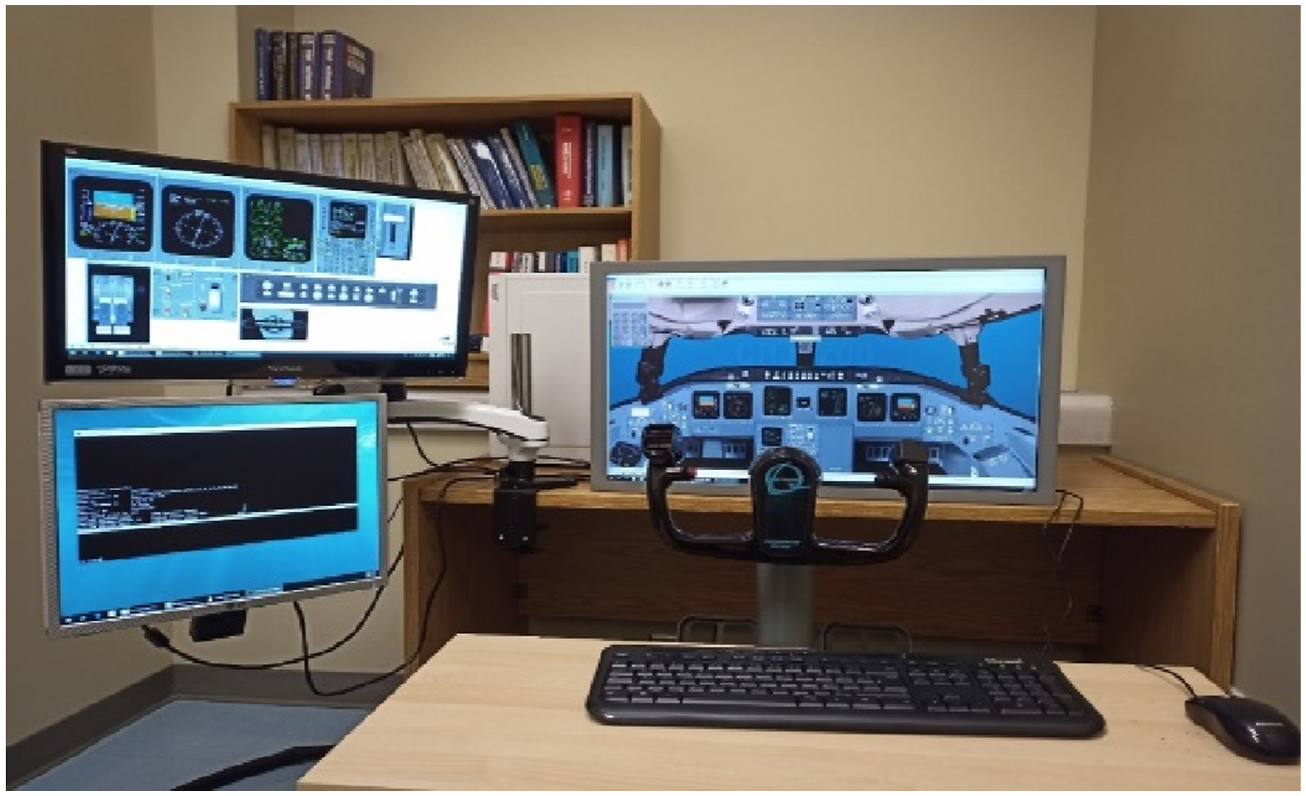
For this research, the engine data obtained from the VRESIM were used as a surrogate with which to compare and calibrate the proposed cycle model. Engine performance data are not readily accessible, given that Original Engine Manufacturers (OEMs) only share such data on a need-to-know basis (e.g., partnership research projects). Moreover, engine experimental data are costly to obtain. Engine performance tests are generally conducted in test cells and require a significant investment to obtain the data: test cell running time, labor, fuel consumption, etc. The approach followed in this research allowed engine data to be obtained in an inexpensive and environmentally friendly fashion, meaning that no actual engine test was performed, instead the data was obtained by using the VRESIM as a proxy. The VRESIM is a research tool (see Figure 1) used at the LARCASE for obtaining both aircraft and engine data.

Figure 1.

High fidelity flight simulator (VRESIM) located at the LARCASE.

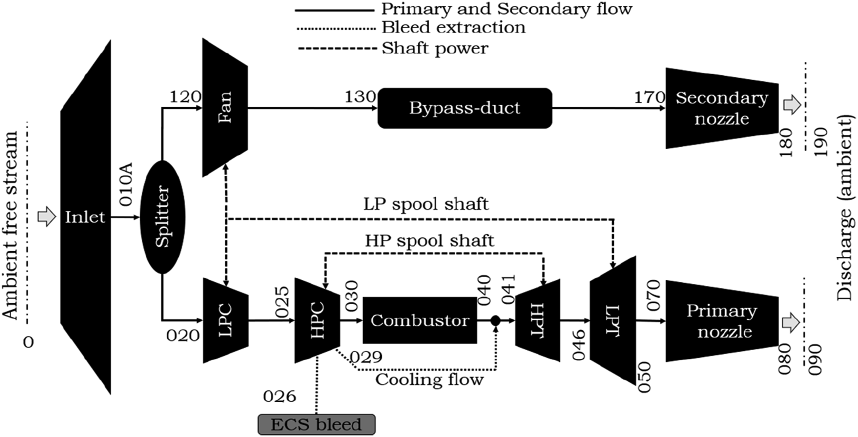
The VRESIM is intended to simulate the CRJ-700 ³¹ which is powered by two General Electric CF34-8C5B1 engines. ³² The CF34-8C5B1 engine is a two-spool, separate exhaust turbofan engine with a normal take-off thrust of 12,670 lb_f (56,359 N). A schematic of this type of engine depicting the major components is presented in Figure 2. The description of each components in Figure 2 and the engine station nomenclature (i.e., the numerals depicted in this figure) are discussed in Ref. 21. The VRESIM encompasses a real-time engine model which can be queried to obtain predetermined data, i.e., only certain high-level performance parameters are available. Real-time engine models are representative of the digital engine model and can reflect, with certain accuracy, the steady-state and transient behaviour of the actual engine. ³³ Based on this assertion, the VRESIM real-time engine model data were deemed representative of the actual CF34-8C5B1 data.

Figure 2.

Separate exhaust turbofan engine schematic.

To fulfill the scope of this research, it was necessary to survey the engine power at different flight conditions. Due to aircraft airworthiness and safety, varying the engine power while maintaining the flight conditions is not achievable on a production aircraft unless it has been modified for such purposes, such as a Flight Test Bed (FTB). FTBs typically have two or three engines that keep the aircraft airborne while allowing to vary the power of the engine subject to analysis. ³⁴ One of the several advantages of using the VRESIM is that it allows engine data collection while trimming the aircraft and maintaining fixed flight conditions (i.e., altitude, aircraft velocity, and temperature). Engine parameters such as net thrust ( $F_n$ ), fuel flow ( ${\dot{m}}_{fuel}$ ), total engine airflow ( ${\dot{m}}_0$ ), and Inter-turbine Temperature ( $ITT$ ) were obtained from the VRESIM runs.

The engineering data obtained from the VRESIM are transient, and thus, suitable Steady State (SS) readings must be computed from the transient data. In this research, an SS reading is defined as the average of the transient performance data over a period of time after thermal stabilization. The transient data obtained from the VRESIM was analyzed to determine the stabilization time required to obtain SS data. Moreover, the SS data were used to establish the throttle sequence procedure (up-vs down-power) for data reproducibility, and finally, to establish if there are any significant engine-to-engine variations (left-vs right-engine).

Aircraft GTE testing is typically performed in ground test facilities (or test cells). During such tests there are two ways of performing the throttle lever excursion, i.e., up-versus down-power. The up-power test consists in moving the throttle (increasing power) by discrete amounts; an example of this type of test is presented in ³⁵ . The test starts at idle and finishes at a high-power condition (e.g., take-off). The engine is allowed to thermally stabilize at each power point to take SS readings. Stabilization time windows used during engine performance testing vary significantly: from three, ³⁶ five^35,37 to as much as 10 min. ³⁶ The latter time window is found in altitude test cells, where the engine is allowed to stabilize for 10 min at the highest power point. It is likely that these stabilization time figures were derived from a compromise between data accuracy and fuel consumption during testing (i.e., cost). In the down-power test, the engine is taken smoothly from idle to high-power and then through varying power settings, finalizing at idle; an example of this test is found in ³⁷ . As with the up-power test, the engine is allowed to dwell at each discrete power point for thermal stabilization.

Regardless of the throttle excursion sequence, the performance of an engine must be verified up-power versus down-power to verify its repeatability and hysteresis. ³⁸ At the beginning of this research, it was unknown if the VRESIM engine model accounts for any reproducibility effect; it therefore needed to be assessed beforehand. Finally, another aspect worth assessing when dealing with engine data installed in an aircraft is to check if observable differences exist between left- versus right-engine. Due to manufacturing differences, no engine is expected to perform exactly as other. Moreover, cockpit readings (such as $ITT$ ) displayed in the simulator showed differences between left- and right-engine, which tend to mimic real performance differences. Thus, it was of paramount importance to determine how the engines compare with each other in case a significant performance difference would have to be addressed.

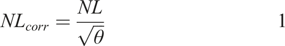
A series of tests were designed and performed to determine thermal stability, data reproducibility, and left-versus right-engine performance differences. The first series was aimed to evaluate the engine in down-power mode, and the second for up-power mode. For each series, four representative power settings were considered, realized by setting the Low-Pressure (LP) corrected speed ( ${NL}_{corr}$ ) defined in equation (1). In this equation, $NL$ is the rotational speed of the LP spool expressed as a percentage of the design rotational speed ( ${NL}_{des}$ ), and $\theta$ is the ratio between the total temperature ( $T_0$ ) at the fan inlet (station 120 in Figure 2) and the standard day temperature $T_{std}=$ 518.67 R (288.15 K). The ${NL}_{corr}$ was set to 100%, 75%, 50%, and about $\approx$ 28% (ground idle setting).

${NL}_{corr}=\frac{NL}{\sqrt{\theta }}$

1

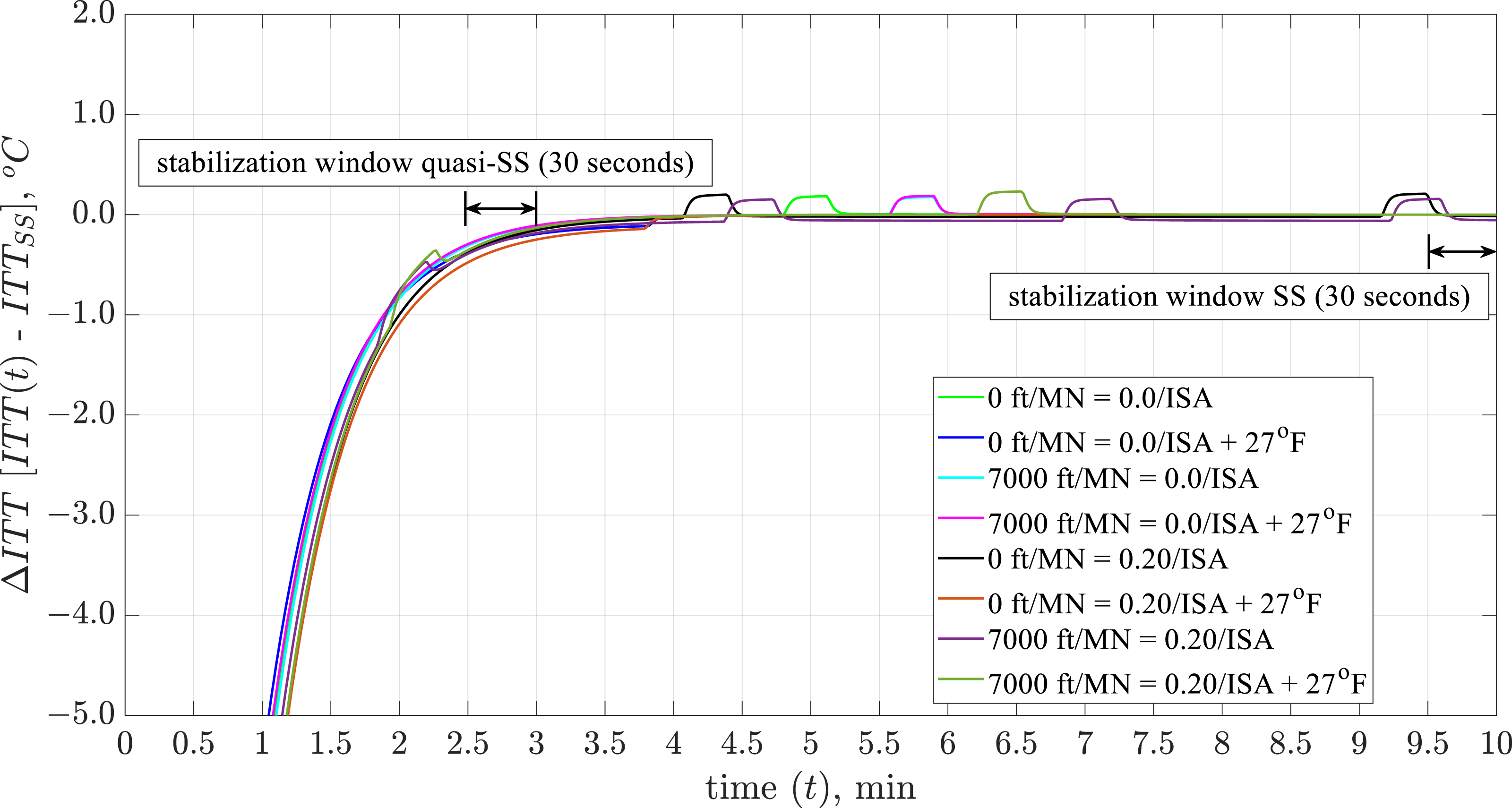
In the up-power series, the engine was left at the idle setting ( ${NL}_{corr}\approx$ 28%) during 60 s before making the throttle excursion to ${NL}_{corr}$ = 100%. For the down-power series, the same power points were considered but in reverse order. At each power point the engines dwelled for 10 min before the throttle was moved to the next power setting. Different flight conditions were tested for both series: altitude at 0 ft and 7000 ft (2134 m); $MN$ at 0.0 and 0.20; and ${∆T}_{ICAO-SA}$ at 0.0 and +27°F (+15°C). The performance parameters assessed during these tests were the $F_n$ , ${\dot{m}}_{fuel}$ , and $ITT$ . Engine thermal stability implies that $\frac{\partial X}{\partial t}=$ 0, where $X$ is any parameter of interest (e.g., $F_n$ , ${\dot{m}}_{fuel}$ , etc.). The thermal stability was assessed using the highest power setting ( ${NL}_{corr}$ = 100%), assuming $\frac{\partial X}{\partial t}=$ 0 is achieved within $∆t$ = 600 s (10 min). For the flight conditions tested, all the parameters but the $ITT$ stabilize almost immediately, i.e., no significant difference between $∆t$ = 0 and $∆t$ = 600 s; $∆t$ = 0 being the time where the target ${NL}_{corr}$ is achieved, and throttle lever is maintained fixed. The $ITT$ shows a lag that takes between $∆t$ = 150 and 180 s to stabilize, as shown in Figure 3. Interestingly, the VRESIM data shows an $ITT$ undershoot, whereas other engine experimental data showed an overshoot. ³⁹ It is also observed that the $ITT$ signals showed some random noise (i.e., small step changes) even after stabilization (for $∆t$ ≥ 4 min). The difference between the $ITT$ values averaged in the 150–180 s window (quasi-SS in Figure 3) and the $ITT$ values averaged 570–600 s window (SS in Figure 3) was less than −0.4°C (−0.72°F). For this study, the quasi-SS window was used to determine data stabilization, with the objective of optimizing the flight tests’ runtime without penalizing $ITT$ accuracy.

Figure 3.

VRESIM $ITT$ transient data at ${NL}_{corr}$ = 100%.

Once the stabilization time was defined, the effect of data reproducibility was assessed. SS readings were computed for the series of flight tests that were tested for up- and down-power conditions. The observed performance differences (up-vs down-power) at constant power-settings were considered negligible. For $F_n$ and ${\dot{m}}_{fuel}$ , the differences were less than ±0.12% and for $ITT$ about ± 2°C. While no significant differences were found between up-versus down-power, the down-power sequence was used to obtain the power lines on each flight tests for the rest of this research work, given that its throttle excursion better approaches a real-life flight mission (going from idle to take-off, to climb and then to idle).

To assess the left-versus right-engine variation, the SS readings for the down-power sequence were compared between both engines at the same power level. Small to negligible differences were observed between them. For ${NL}_{corr}$ = 100%, 75% and 50%, the $ITT$ differences were less than 0.5°C, whereas for ${\dot{m}}_{fuel}$ the greatest error observed was $\approx$ 0.10%. For the idle setting, the $\mathrm{\Delta }ITT$ increased to about 1.0°C and 0.4% for ${\dot{m}}_{fuel}$ . The $F_n$ showed negligible differences across power-settings. Despite the small to negligible engine-to-engine differences, the performance outcome of both engines was averaged to be used for comparison/matching with the cycle model.

Flight test data for model matching

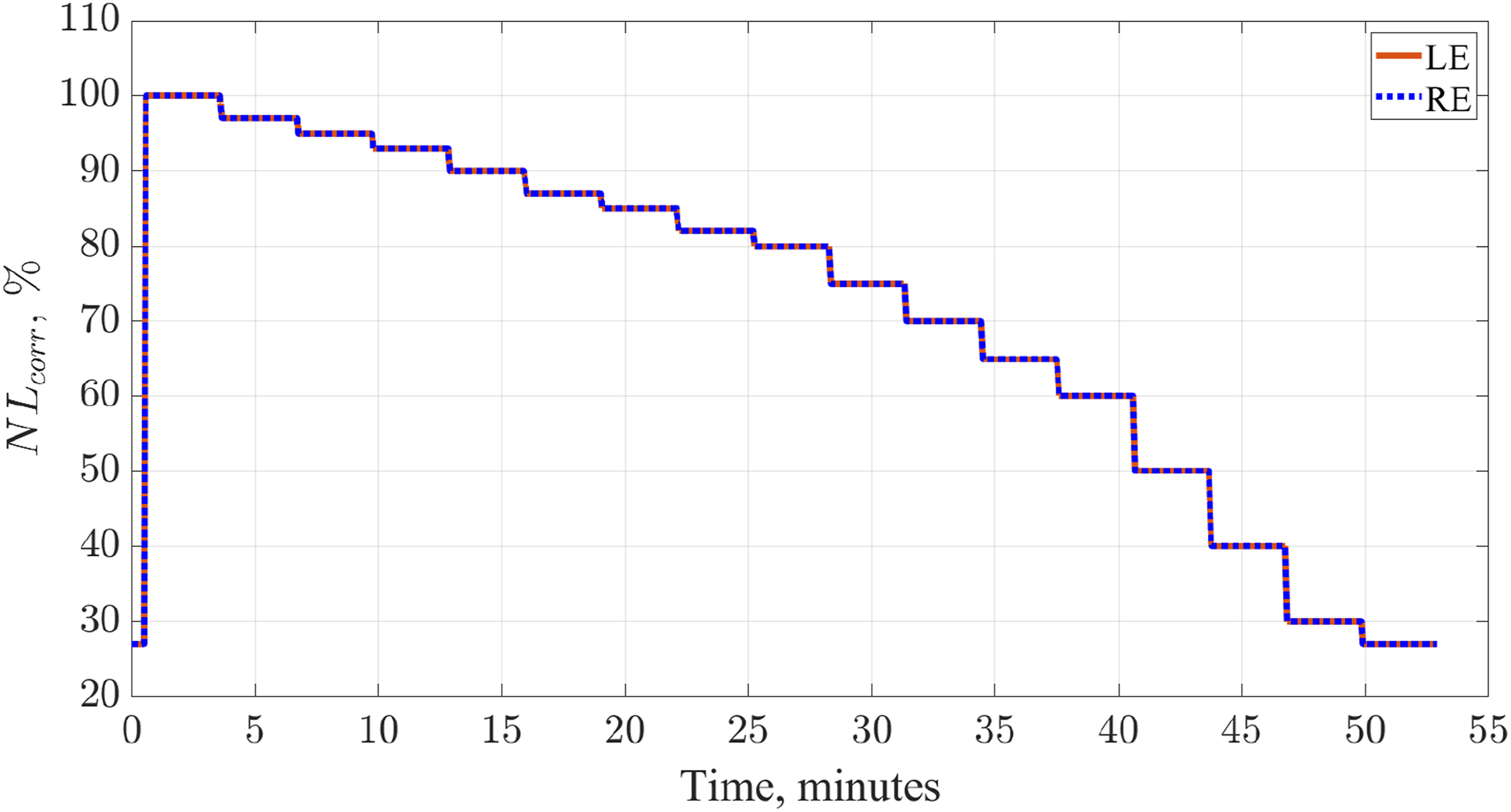
This section discusses the flight tests for model calibration. A comprehensive survey of data points, from high to idle power, on each flight condition was conducted, as shown in Figure 4. For ${NL}_{corr}$ ≥ 80%, the data points were obtained at ${∆NL}_{corr}$ = 2.5%; for 60 ≤ ${NL}_{corr}$ < 80% at ${∆NL}_{corr}$ = 5.0%. Finally, for ${NL}_{corr}$ < 60% at ${∆NL}_{corr}$ = 10%. Concerning minimum idle power point, the engine control regulates the power to keep ${NL}_{corr}\approx$ 28%. Finally, the VRESIM scan rate was set to 1 Hz.

Figure 4.

Engine power excursion during flight tests (LE: left-engine, RE: right-engine).

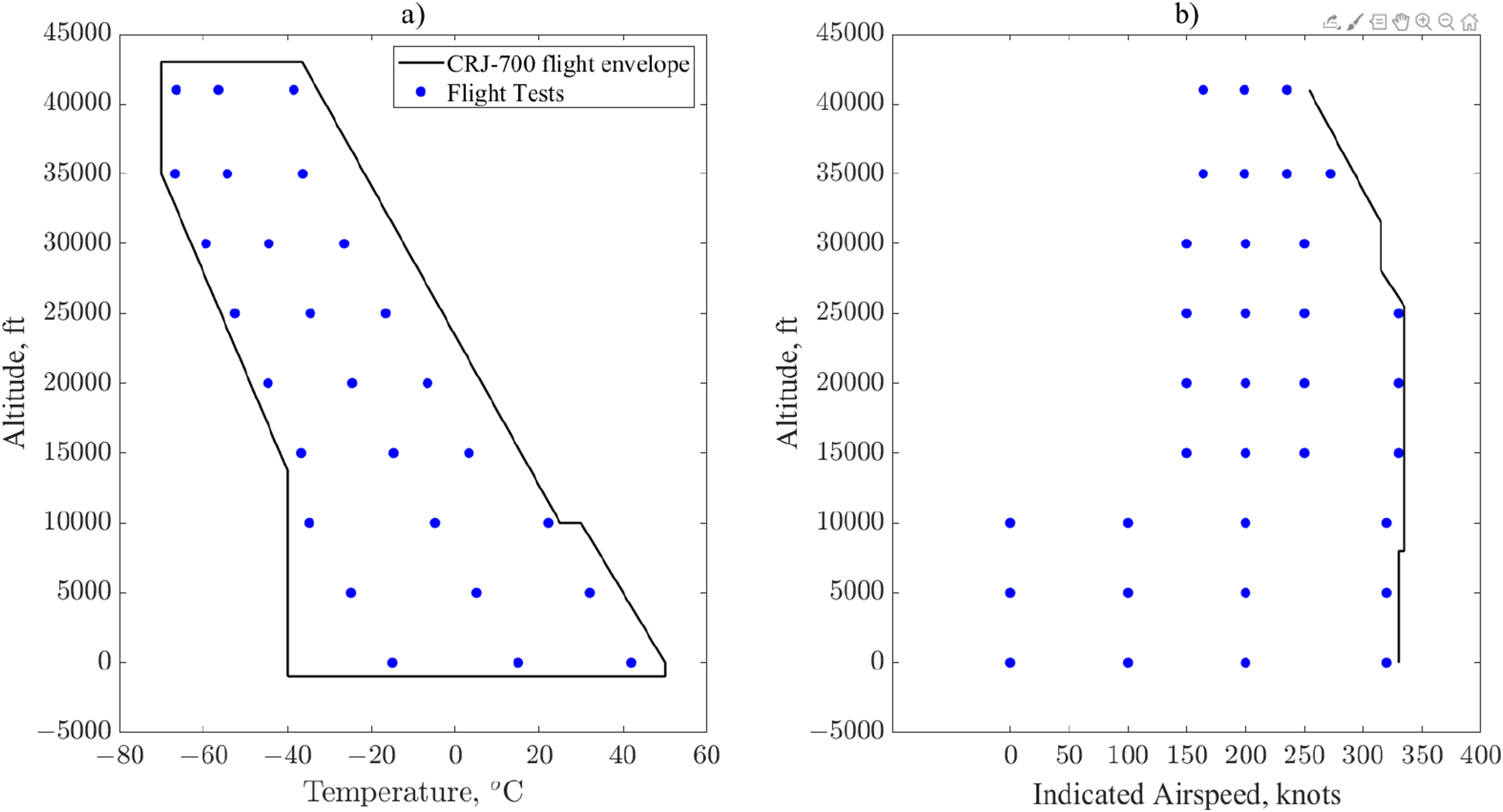
The power survey was run across different flight conditions within the CRJ-700 flight envelope ⁴⁰ depicted in Figure 5. The flight conditions accounted for nine discrete levels of altitude (L1−L9) which encompass low to high altitudes. At each altitude, six flight velocities’ (IAS, Indicated Airspeed) levels were sampled, and various temperature deviations from ISA (International Standard Atmosphere) were considered ( ${∆T}_{ICAO-SA}$ ). However, these ${∆T}_{ICAO-SA}$ were not constant across altitude levels due to envelope or engine operational limitations. The total number of data points considered in this work were 1468, from which 60 were used for initial model comparison and calibration, and the remaining 1408 were used for final model validation.

Figure 5.

Flights tests for engine calibration and validation: (a) thermal envelope and (b) speed envelope (axes numeric values are not presented due to proprietary information reasons).

The cycle model and the matching process

Two versions of the engine cycle model were generated in this research. The first version, the baseline model (CM-8C5B1-Base), was assembled considering the assumptions (i.e., the ADP) established by Gurrola Arrieta and Botez. ²¹ The second version, the final matched model (CM-8C5B1), was obtained by calibrating the CM-8C5B1-Base to the VRESIM data at predefined flight conditions and power-settings. More details about these two models are discussed next.

The CM-8C5B1-Base is an Off-Design (OD) cycle model. OD models are used to predict the performance of a fixed-size engine throughout different power regimes and flight conditions. The CM-8C5B1-Base was built using the so-called Aerothermodynamic Generic Cycle Model (AGCM), a high-fidelity, zero-dimensional, SS model in MATLAB developed in-house at the LARCASE. ²¹ The ADP developed in Ref. 21 encompasses the necessary assumptions (bypass ratio, turbomachinery adiabatic efficiencies, fuel properties, total engine flow, etc.) to define the exhaust flow areas of the primary and secondary nozzles ( $A_{080}$ and $A_{180}$ ), as well as the turbomachinery maps scaling factors. The area ratio (secondary to primary) obtained by these ADP assumptions was $A_{180}/A_{080}$ = 3.9. However, the turbomachinery maps used in this research were different from those considered in Ref. 21 and their scaling factors were close to unity, whereas the ones from, ²¹ overall differ significantly from unity. These flow areas and scaling factors defined the CM-8C5B1-Base.

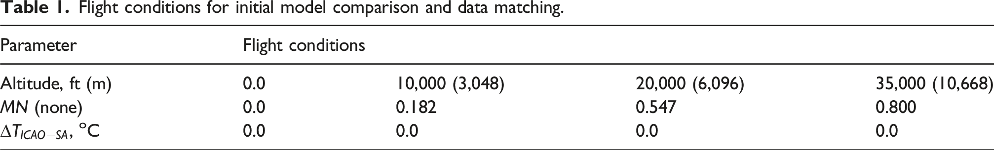
The CM-8C5B1-Base was then compared to the VRESIM. First, simulations were run on both of them at representative flight conditions, listed in Table 1, which are within the data points depicted in Figure 5. At each of these flight conditions, the power sweep depicted in Figure 4 was executed. However, for the CM-8C5B1-Base, some of the lower power points were not reached, e.g., at sea-level about ${NL}_{corr}$ = 28% and at high altitude for ${NL}_{corr}$ < 40%. The operating points in these regions tend to be outside the CM-8C5B1-Base fan map’s domain, and so the numerical method cannot find a valid solution. To avoid convergence problems, the lower end of the ${NL}_{corr}$ was constrained to the closest value in which the model can attain a solution. Next, the results from these runs were compared. These comparisons served as a verification of the ADP’s fitness. The best way to ensure the ADP assumptions are reasonable is to compare them with the engine data. This initial check helped to revise some assumptions, such as total engine airflow ( ${\dot{m}}_0$ ), as discussed in the Results and discussion section. The CM-8C5B1-Base was then tuned (calibrated) to match the data at the flight conditions shown in Table 1.

Table 1.

Flight conditions for initial model comparison and data matching.

Parameter	Flight conditions
Altitude, ft (m)	0.0	10,000 (3,048)	20,000 (6,096)	35,000 (10,668)
MN (none)	0.0	0.182	0.547	0.800
${∆T}_{ICAO-SA}$ , oC	0.0	0.0	0.0	0.0

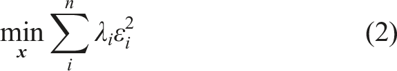
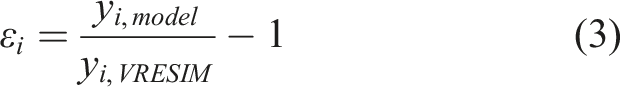
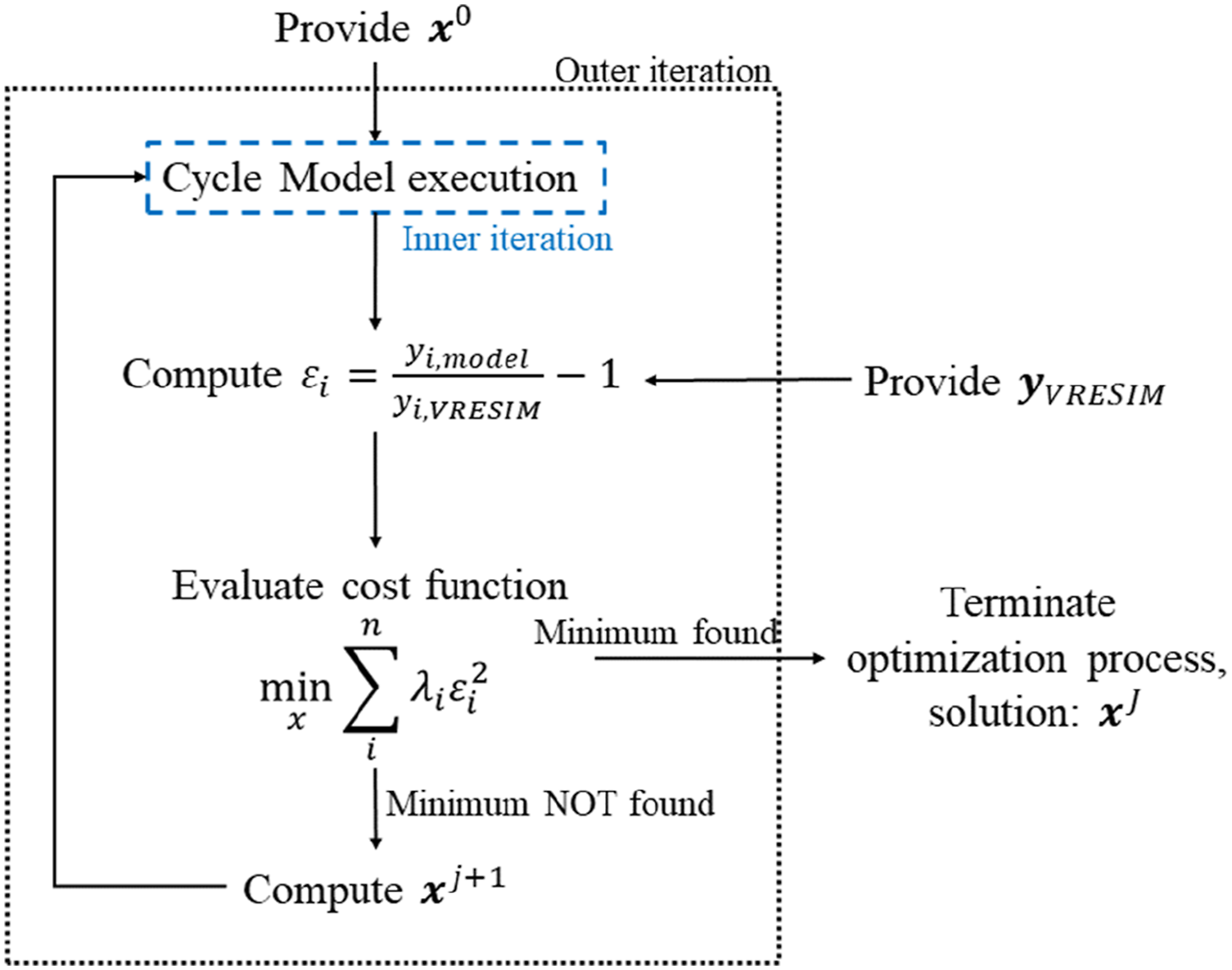
The model calibration was based on an optimization process in which the errors ( $\epsilon$ ) between the cycle model and the VRESIM were minimized by changing the model’s independent parameters (x). The optimization problem is expressed in equation (2). The objective (cost) function in equation (2) is defined as the weighted sum of the squares of the errors between the dependent parameters ( $y$ ), as defined in equation (3). In equation (2), $\lambda$ is the desired weighting factor. The dependent parameters’ vector, $\mathit{y}={\left[y_1,y_2\right]}^T$ , encompasses the key parameters on this research $y_1=F_n$ and $y_2={\dot{m}}_{fuel}$ , whereas for the independent parameters, $\mathit{x}={\left[x_1,x_2\right]}^T$ includes the fan speed reposition in the map ( $x_1=\delta N_{120,corr}$ ) and the Low-Pressure Turbine (LPT) map adiabatic efficiency adjustment ( $x_2=\delta {\eta }_{LPT}$ ). Finally, it is worth noting that the cost function was minimized at each discrete ${NL}_{corr}$ level presented in Figure 4.

$\underset{\mathit{x}}{\min }{\displaystyle \sum }_i^n{\lambda }_i{\epsilon }_i^2$

(2)

where,

${\epsilon }_i=\frac{y_{i,model}}{y_{i,VRESIM}}-1$

(3)

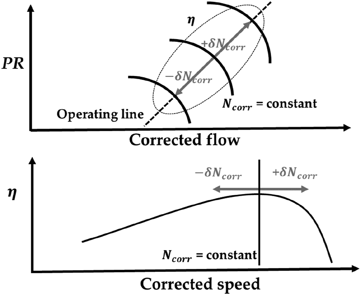
The choice of the parameters that constitute x were selected based on the physics of the problem, which is discussed next. The $F_n$ value depends on the inlet flow linear momentum and the gross thrust produced by both the primary ( $F_{g,pri}$ ) and secondary ( $F_{g,\mathit{sec}}$ ) nozzles. Provided that the inlet momentum is fixed, the thrust production relies on both gross thrusts. The value of $F_{g,pri}$ is significantly affected by the total exit temperature of the hot gas: for a fixed nozzle $\mathit{PR}$ and flow area ( $A$ ), higher total temperatures produce higher jet exhaust velocities, which increase $F_{g,pri}$ . The total temperature at the exit of the primary nozzle ( $T_{0,080}$ ) is affected by the efficiencies of the primary stream components, one of which is the LPT. Indeed, other component efficiencies may affect $T_{0,080}$ (and hence $F_{g,pri}$ ), but the process of choosing the LPT efficiency will become obvious later, when discussing the effect of fuel flow. Moreover, $F_{g,\mathit{sec}}$ is considerably driven by the fan performance, i.e., by the corrected flow, the $\mathit{PR}$ , and the adiabatic efficiency ( $\eta$ ). When repositioning the map speed lines ( $\delta N_{120,corr}$ ) over the same compressor operating line, all these parameters are impacted. A + $\delta N_{120,corr}$ repositions any given speed line towards the up-right of the map, increasing both the corrected flow and the $\mathit{PR}$ . Conversely, $-\delta {NL}_{corr}$ shifts the speed to the lower-left, reducing both the corrected flow and the, as depicted in Figure 6 (top). The behaviour of efficiency (increase/decrease) cannot easily be deduced given that $\eta$ is not monotonic with respect to $\delta N_{120,corr}$ (Figure 6, bottom).

Figure 6.

Effect of fan map speed lines’ repositioning. Top: pressure ratio versus corrected flow; adiabatic efficiency versus corrected rotational speed.

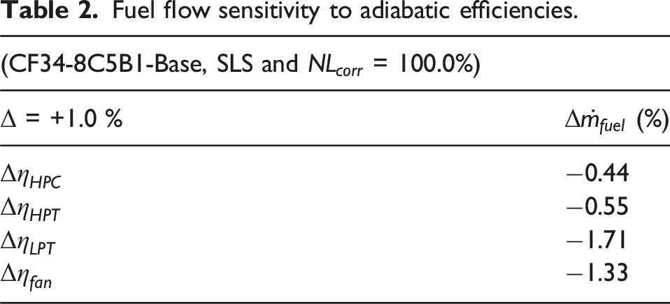
On the other hand, ${\dot{m}}_{fuel}$ is also significantly affected by $\delta N_{120,corr}$ , since it affects the amount of work required by the fan. Furthermore, ${\dot{m}}_{fuel}$ is more sensitive to low-pressure than high-pressure system component efficiency changes ( $\mathrm{\Delta }\eta$ ). The ${\dot{m}}_{fuel}$ sensitivity to adiabatic efficiencies is presented in Table 2, which indicates the significant impact of both LPT and fan efficiencies compared to those in the HPT and HPC. For example, to produce $∆{\dot{m}}_{fuel}$ = +1.0%, the $∆{\eta }_{HPT}$ must be 3.1 times greater than $∆{\eta }_{LPT}$ . It is also worth noting that changes in both fan and LPT adiabatic efficiencies produce similar impacts on $∆{\dot{m}}_{fuel}$ , i.e., $\frac{∆{\dot{m}}_{fuel}}{\mathrm{\Delta }{\eta }_{fan}}\approx \frac{∆{\dot{m}}_{fuel}}{\mathrm{\Delta }{\eta }_{LPT}}$ . The $∆{\eta }_{LPT}$ was selected over $∆{\eta }_{fan}$ because the fan efficiency is already affected by $\delta N_{120,corr}$ . Furthermore, the LPT efficiency affects both ${\dot{m}}_{fuel}$ and $F_{g,pri}$ , whereas fan efficiency affects ${\dot{m}}_{fuel}$ and $F_{g,\mathit{sec}}$ . Had $\mathrm{\Delta }{\eta }_{fan}$ been considered for the matching process, then the errors in net thrust would be solely dependent upon the gross thrust of the secondary nozzle, i.e., ${\epsilon }_{F_n}=f\left(F_{g,\mathit{sec}}\right)$ . Instead, considering $\mathrm{\Delta }{\eta }_{LPT}$ , these errors depend on both gross thrusts, ${\epsilon }_{F_n}=f\left(F_{g,\mathit{sec}},F_{g,pri}\right)$ .

Table 2.

Fuel flow sensitivity to adiabatic efficiencies.

(CF34-8C5B1-Base, SLS and ${NL}_{corr}$ = 100.0%)
$\mathrm{\Delta }$ = +1.0 %	$\mathrm{\Delta }{\dot{m}}_{fuel}$ (%)
$\mathrm{\Delta }{\eta }_{HPC}$	−0.44
$\mathrm{\Delta }{\eta }_{HPT}$	−0.55
$\mathrm{\Delta }{\eta }_{LPT}$	−1.71
$\mathrm{\Delta }{\eta }_{fan}$	−1.33

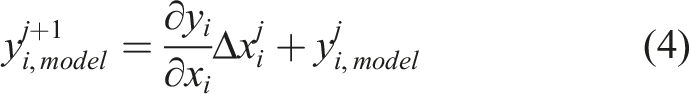
The weighting factors ( $\lambda$ ) for the $F_n$ and ${\dot{m}}_{fuel}$ errors in equation (2) were 0.7 and 0.3, respectively. Due to data quality concerns, a lower weighting factor was given to ${\dot{m}}_{fuel}$ , which will be further discussed in the Results and discussion section. The optimization process outlined in this research requires computing an updated ${\mathit{y}}_{model}^{j+1}$ at each j-iteration. To do this, the cycle model has to be run at every j-iteration with updated values of ${\mathit{x}}^j$ . Moreover, this process needs to be repeated for each ${NL}_{corr}$ , which generates two challenges that made the optimization process inefficient and time consuming. First, the cycle model is an iterative process on its own; it has to iterate to resolve the imbalances in mass and energy within the thermodynamic cycle for each value of ${\mathit{x}}^j$ , generating a nested iteration process, as depicted in Figure 7. The outer iteration corresponds to the optimization process execution, and the inner one is for solving the thermodynamic cycle imbalances. Second, large $∆\mathit{x}$ could cause the cycle model to crash or encounter convergency issues. To circumvent the challenges identified above, a simplified performance model representation was proposed. This simplified representation assumes a linear behavior of $y_{i,model}$ within a relatively small change of $∆x_i$ as expressed in equation (4). The main advantage of this simplified model is that it only requires independent cycle model runs to compute the initial values (j = 0) for $y_{i,model}$ , $\mathrm{\Delta }{x}_i$ , and the partial derivatives ( $\frac{\partial y_i}{\partial x_i}$ ). These derivatives are a function of ${NL}_{corr}$ and the flight $MN$ , and remained constant throughout the matching process. The introduction of the linear model thus overcame the problems discussed above.

$y_{i,model}^{j+1}=\frac{\partial y_i}{\partial x_i}∆x_i^j+y_{i,model}^j$

(4)

Figure 7.

Cycle model match process. Inner loop, cycle model execution to resolve cycle mass and energy imbalances; outer loop, matching process.

The final matched model (CM-8C5B1) was run at the flight conditions shown in Figure 5 to calculate the errors ( $\epsilon$ ) in $F_n$ and ${\dot{m}}_{fuel}$ ; however, at this stage, additional performance parameters were also evaluated, such as the total engine airflow ( ${\dot{m}}_0$ ) and the $ITT$ . The ${\dot{m}}_0$ is a helpful performance parameter that is highly correlated to the $F_n$ , and is therefore used for diagnostic purposes. The $ITT$ is the average temperature of the hot gases and plays a significant role in engine health monitoring. This temperature is measured by an array of five or 20 thermocouples mounted in the LPT casing. ³² The $ITT$ signal readings are displayed in the cockpit in real time, and they are an indication of how hot the engine is running. Pilots are mandated to monitor $ITT$ and to take actions in case safety limits, called redlines, are exceeded. As stated in the Introduction section, both ${\dot{m}}_0$ and $ITT$ were excluded from the matching process, as they were not central to the objectives of this research. The CM-8C5B1’s predictions for these parameters are a byproduct of enhancing the accuracy of thrust and fuel flow. However, as will be discussed in the next section, the accuracy of ${\dot{m}}_0$ appears to align with that of fuel flow and thrust.

Results and discussion

Design point evaluation

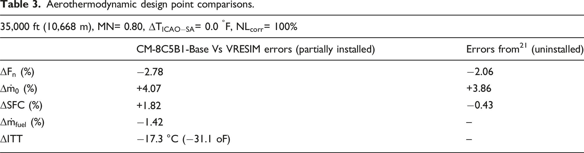
During ongoing research, the Aerothermodynamic Design Point (ADP) of an already-designed engine is rarely known. This information is proprietary to the OEMs, and hence not publicly available. Nonetheless, engineers and scientists often seek to determine an approximation of what they believe the ADP of a given application would be based on engine marketing data and open literature information, and on their best engineering judgement, as in Ref. 21. The assumptions for defining the ADP include the specific flight conditions (altitude, $MN$ , ambient temperature, power-setting) and the thermodynamic cycle design assumptions (e.g., $\beta$ , $\eta$ , $\mathrm{\Delta }\mathrm{P}/P$ , etc.). During the following discussion, when the ADP is referred to, it should be understood as the authors’ approximation of the CF34-8C5B1 ADP. In a previous work, Gurrola Arrieta and Botez ²¹ presented a preliminary assessment of the ADP fitness; nonetheless, this assessment was done based on comparisons with other engines of similar size/thrust. Such assessment considered uninstalled performance, i.e., no HPC bleed extraction for aircraft cabin ventilation, and no pressure loss for inlet and bypass ducts. For the present study, first, the engine was sized considering its uninstalled performance as in Ref. 21. Second, both OD models were adjusted to account for inlet and bypass duct-normalized pressure losses ( $\mathrm{\Delta }P/P$ ) but still considering there was no HPC bleed extraction for aircraft cabin ventilation, i.e., partially installed. These adjustments were performed because it was deemed that the real-time engine model in the VRESIM encompasses these pressure losses, and they cannot be altered. The inlet and bypass duct pressure recovery were set to $∆{P/P}_{inlet-duct}$ = 0.34% and $∆{P/P}_{bypass-duct}$ = 2.4%. ²¹ These assumptions ( $\mathrm{\Delta }P/P$ and no HPC bleed extraction for cabin ventilation) remain invariant throughout further comparisons in this work. Finally, the ADP assessment was performed, as in Ref. 21 at 35,000 ft (10,668 m), 0.80 Mach, and standard day temperature ( $\mathrm{\Delta }{T}_{ICAO-SA}$ = 0.0), running at ${NL}_{corr}$ = 100% (i.e., top of climb). The results of these comparisons are presented in Table 3 along with those from. ²¹ It is noteworthy that the $\mathrm{\Delta }{\dot{m}}_{fuel}$ and $∆ITT$ are not discussed in Ref. 21 thus not displayed in Table 3.

Table 3.

Aerothermodynamic design point comparisons.

35,000 ft (10,668 m), $\text{MN}$ = 0.80, ${∆\mathrm{T}}_{\text{ICAO}-\text{SA}}$ = 0.0 °F, ${\text{NL}}_{\text{corr}}$ = 100%
	CM-8C5B1-Base Vs VRESIM errors (partially installed)	Errors from 21 (uninstalled)
${\mathrm{\Delta }\mathrm{F}}_{\mathrm{n}}$ (%)	−2.78	−2.06
${∆\dot{\mathrm{m}}}_0$ (%)	+4.07	+3.86
$\mathrm{\Delta }\text{SFC}$ (%)	+1.82	−0.43
$\mathrm{\Delta }{\dot{\mathrm{m}}}_{\text{fuel}}$ (%)	−1.42	–
$\mathrm{\Delta }\text{ITT}$	−17.3 °C (−31.1 oF)	–

The errors observed between ²¹ and the present work are of a similar order of magnitude as those depicted in Table 3. Both the present study and in Ref. 21 the $SFC$ errors were computed at constant predefined $F_n$ rather than at ${NL}_{corr}$ . For the present study, the $F_n$ corresponds to the CM-8C5B1-Base at ${NL}_{corr}$ = 100%. The errors in Table 3 (second column) are within the desired accuracy for validating the model (i.e., ± 5.0%), and suggest the assumptions established in Ref. 21 are a realistic estimate of the CF34-8C5B1 ADP.

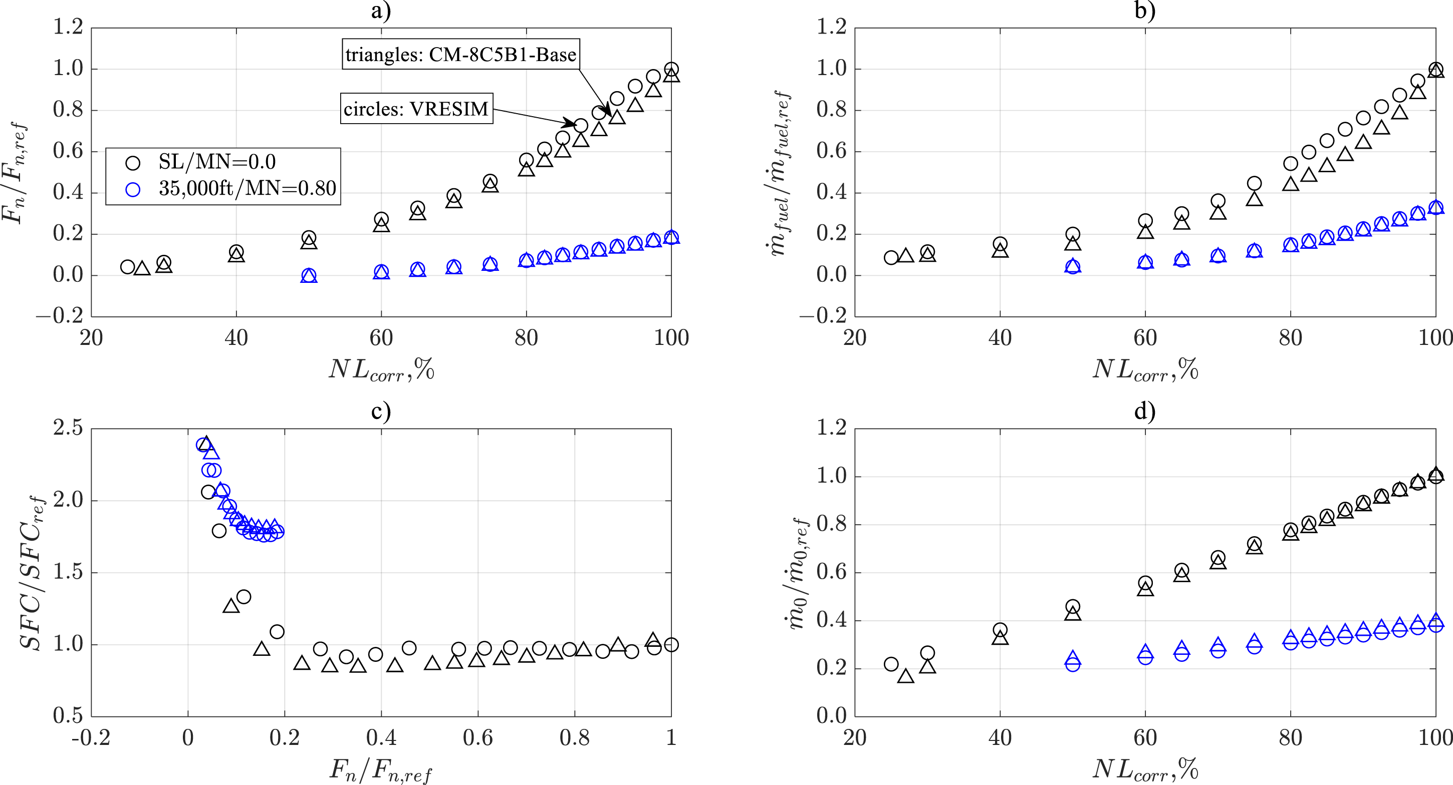
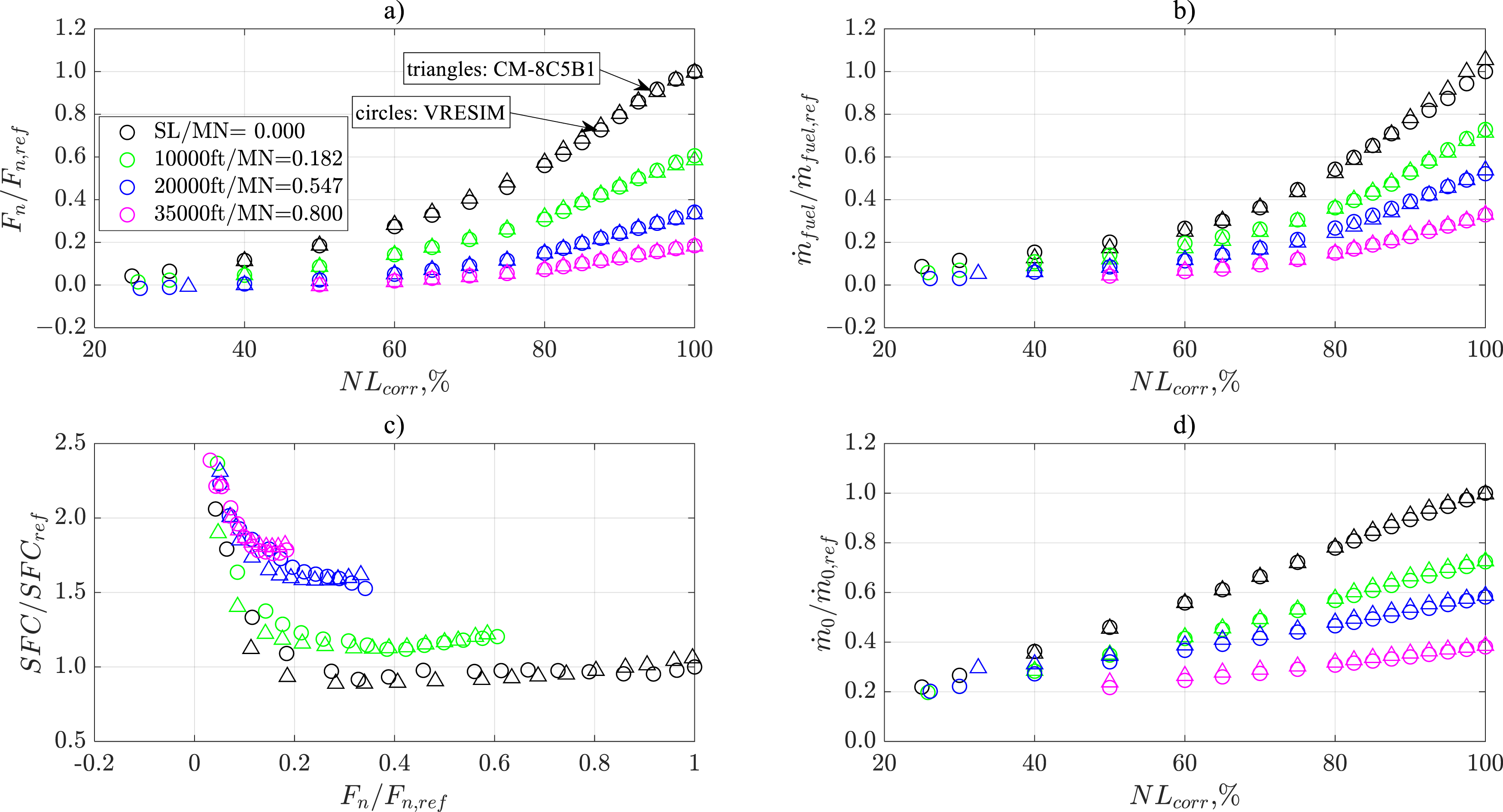
The comparison between the CM-8C5B1-Base and the VRESIM was expanded for other power-settings ( ${NL}_{corr}$ ) and flight conditions, namely Sea-Level Static (SLS) and 35,000 ft (10,668 m)/ $MN$ = 0.80. The comparisons are shown in Figure 8 for normalized $F_n$ , ${\dot{m}}_{fuel}$ , $SFC$ , and ${\dot{m}}_0$ . The normalization was performed taking as reference the values from the VRESIM at SLS and ${NL}_{corr}$ = 100.0%; at this condition, the normalized VRESIM data are equal to 1.0. As observed in Figure 8, the CM-8C5B1-Base’s performance resembles the VRESIM trends throughout various power-settings for both flight conditions. However, fuel flow (Figure 8(b)) presents a significant mismatch at SLS between ${NL}_{corr}$ = 80%-90%. One observation to add to this discussion is that the VRESIM-normalized $SFC$ values present a none-smooth behaviour for SLS. Typically, $SFC$ versus $F_n$ curves from cycle models tend to show a smooth concave function, i.e., a bucket-shape type. In Figure 8(c)), the CM-8C5B1-Base data shows a minimum about $F_n/F_{n,ref}$ = 0.35 and then monotonically increases towards the left or right. With the VRESIM, however, after reaching the minimum $F_n/F_{n,ref}$ = 0.325, the normalized $SFC$ do not increase monotonically towards the right.

Figure 8.

Normalized performance CM-8C5B1-Base versus VRESIM: (a) thrust; (b) fuel flow; (c) $SFC$ ; (d) airflow.

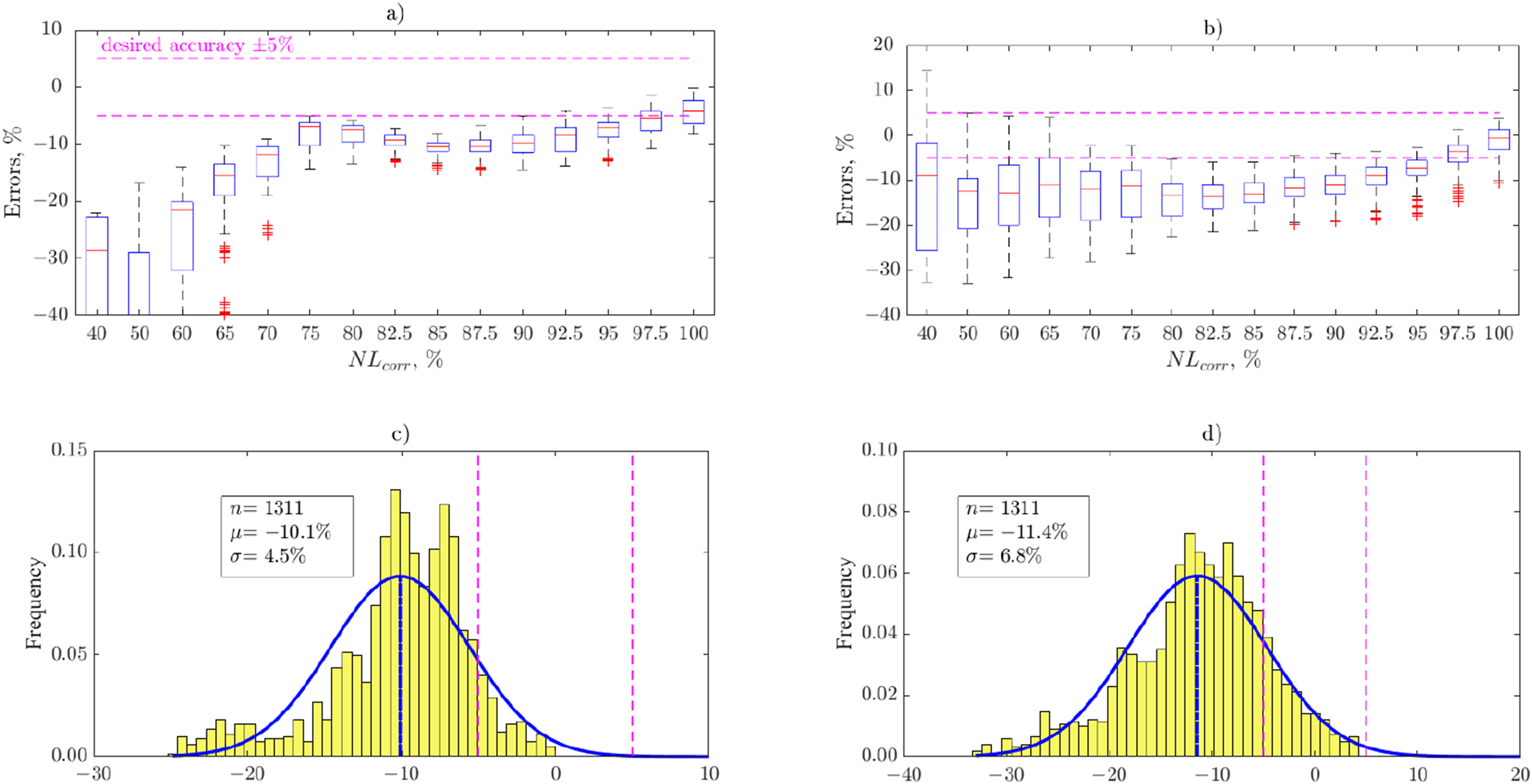
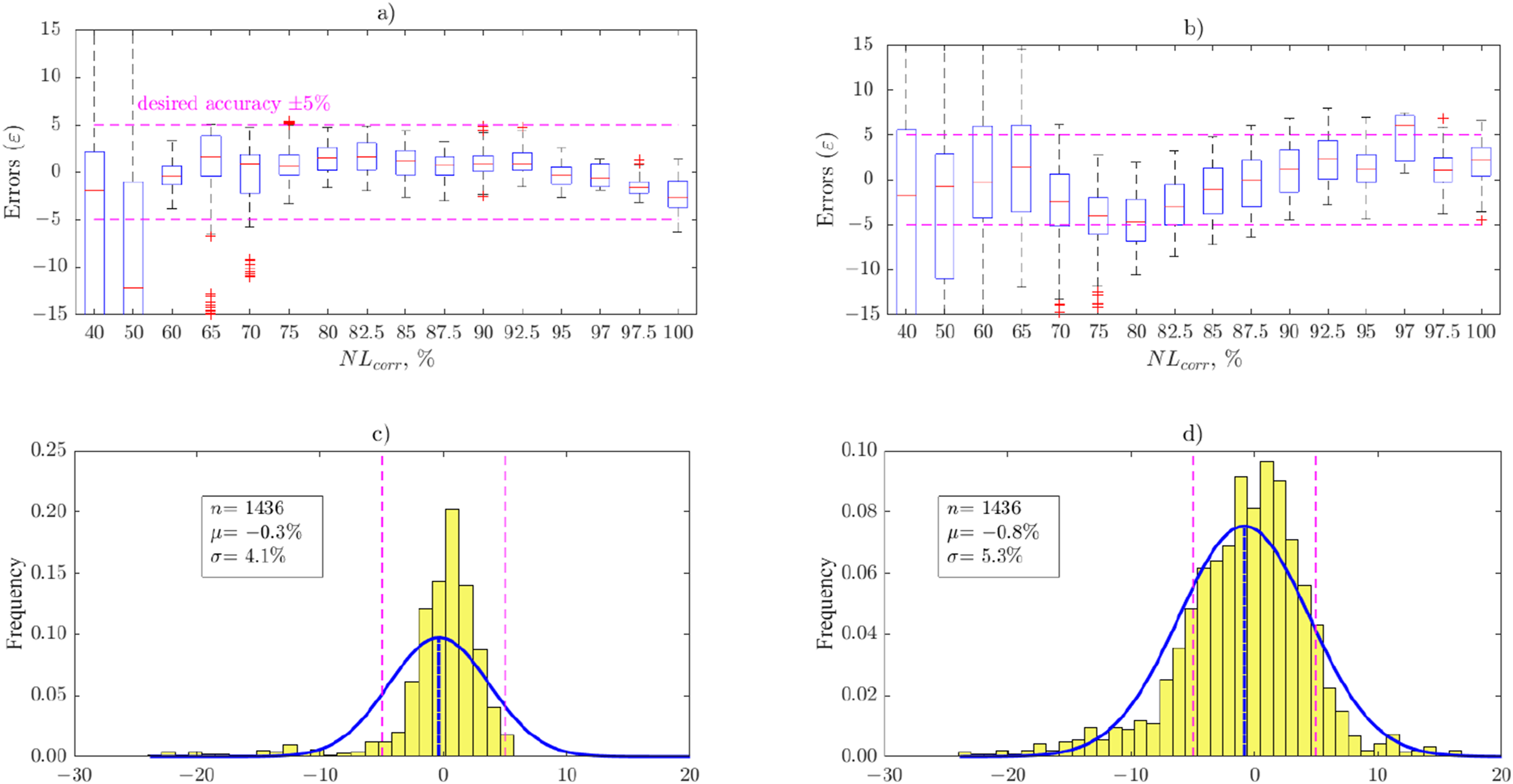
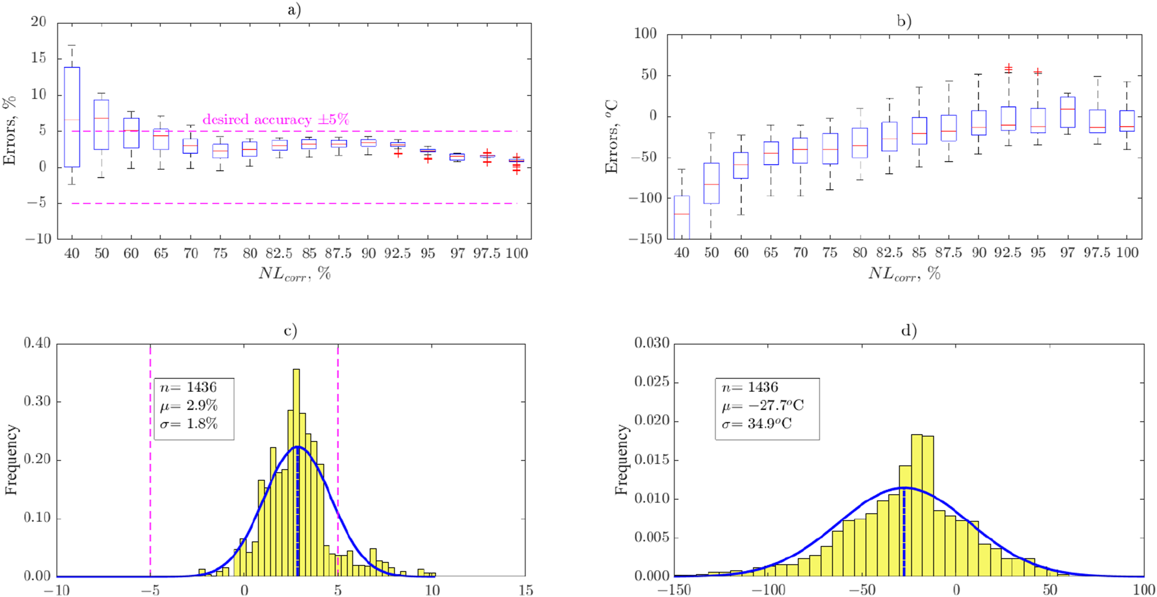
A more thorough comparison between the CM-8C5B1-Base and the VRESIM is presented in Figure 9, in which the full set of validation flight tests (Figure 5) is considered. In Figure 9, the same information is presented in two different ways. The boxplots of ε versus ${NL}_{corr}$ are shown in Figure 9(a) and (b), and their corresponding histograms in Figure 9(c) and (d). While histograms are typically used for depicting error distribution, they could portray an incomplete representation for the type of comparisons presented in this paper because they only provide a global view of the errors’ scatter. For example, looking at the thrust error histogram (Figure 9(c)), the conclusion that can be drawn is that the errors tend to follow a normal distribution with an average ( ${\mu }_{F_n}$ ) of −10.1%, and a large standard deviation ( ${\sigma }_{F_n}$ = 4.5%). However, observing the boxplot errors versus ${NL}_{corr}$ (Figure 9(a)), it is evident that, at constant ${NL}_{corr}$ , the scatter of the errors and their averages are considerably lower than the overall error. For example, at ${NL}_{corr}$ = 100%, ${\mu }_{F_n}$ = −4.0 and ${\sigma }_{F_n}$ = 2.3%. It is worth noting there are individual errors not shown in Figure 9(a) and (b) given that, for low power-settings, both these errors become significantly large, making it difficult to appreciate and interpret the data. Also, in Figure 9(c) and (d), the data and statistics in the histograms are presented for ${\epsilon }_{F_n}$ = ±25.0%, which help us to focus our results discussion inasmuch as the statistics are very sensitive to extreme values (or outliers).

Figure 9.

CM-8C5B1-Base versus VRESIM errors. (a) $F_n$ errors versus ${NL}_{corr}$ ; (b) ${\dot{m}}_{fuel}$ errors versus ${NL}_{corr}$ ; (c) $F_n$ errors histogram; (d) ${\dot{m}}_{fuel}$ errors histogram.

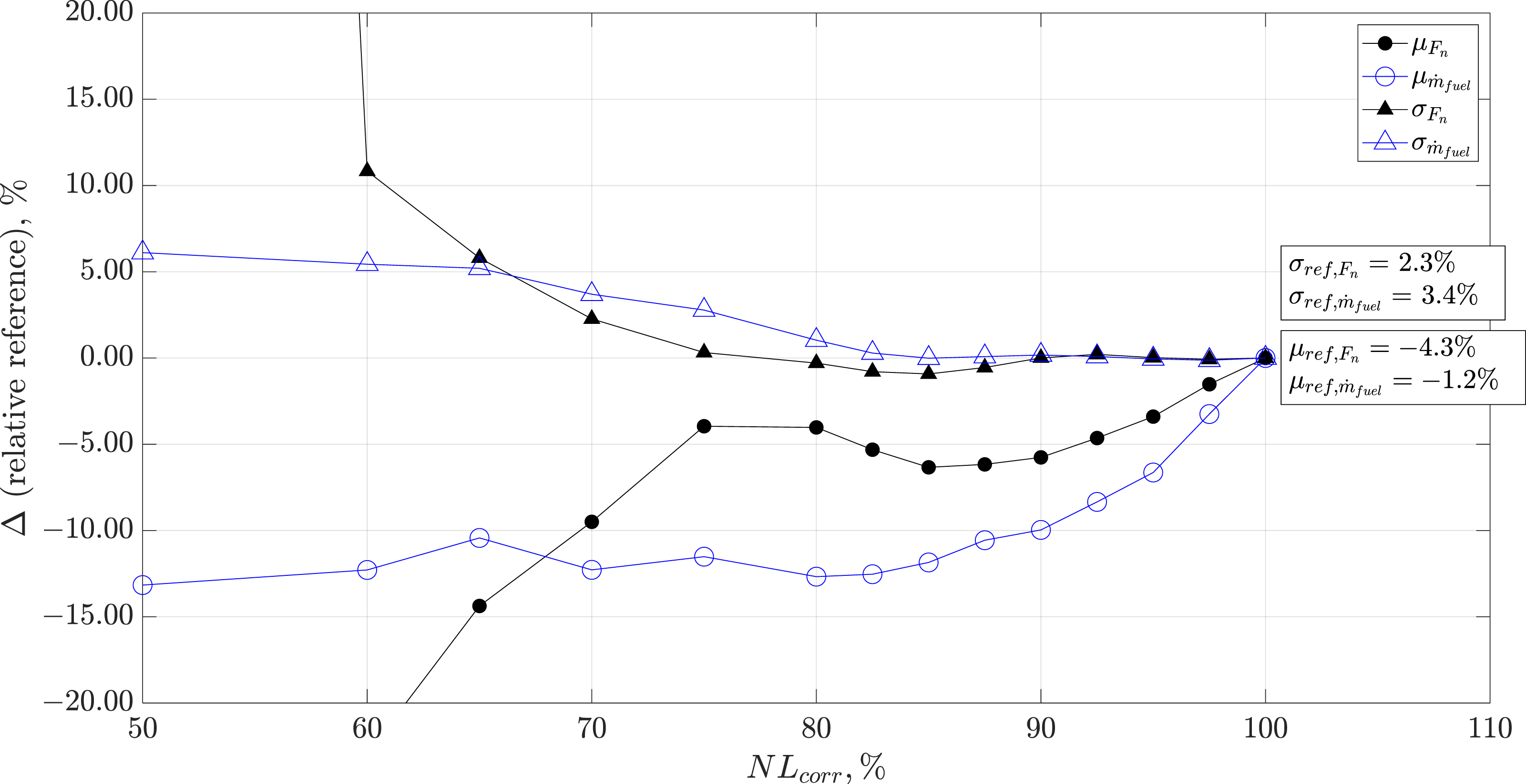
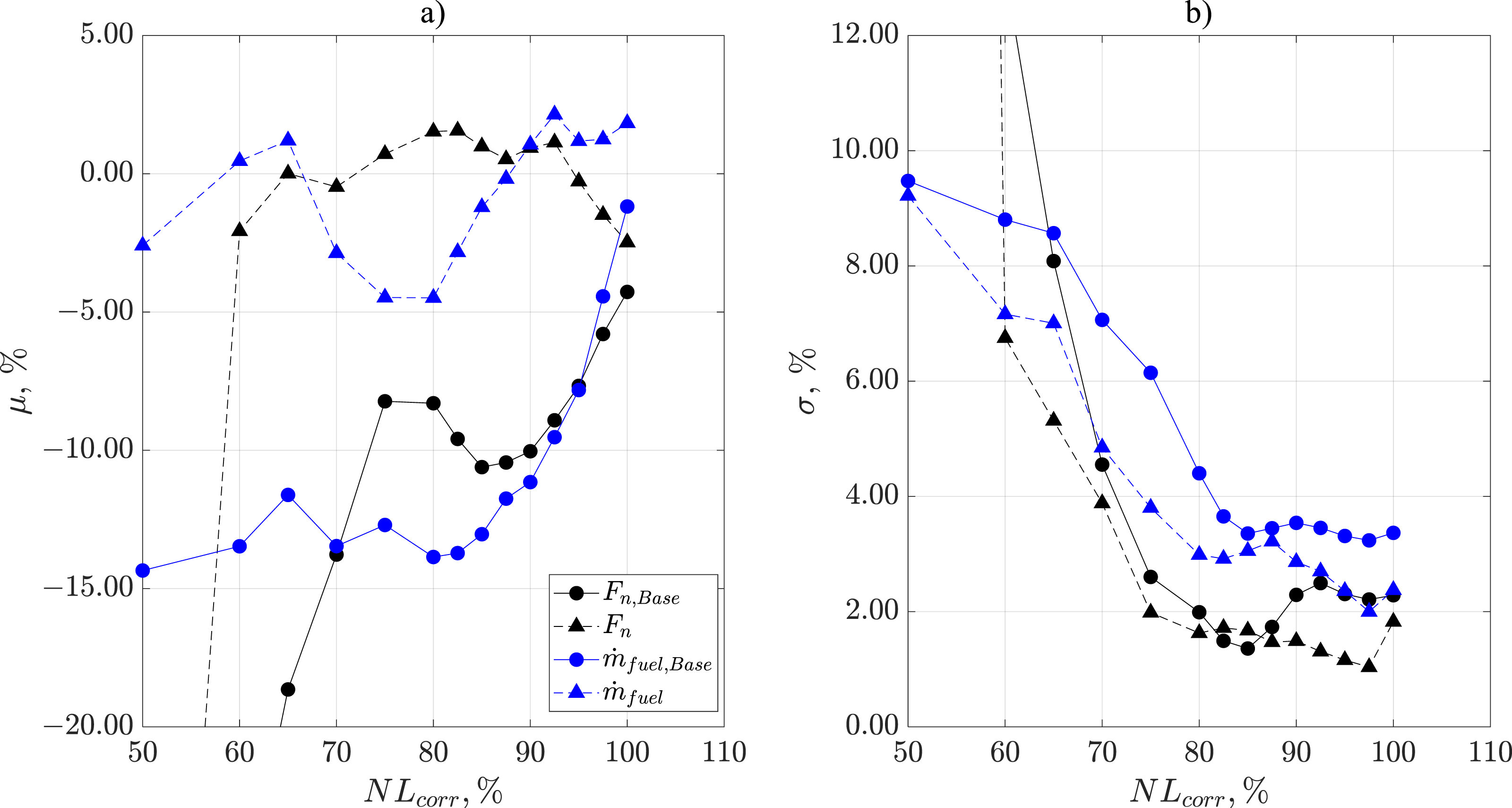
The normalized averages and standard deviations of the errors are presented in Figure 10. The normalized $F_n$ and ${\dot{m}}_{fuel}$ averages are both significantly biased towards the negative side across power-settings. In other words, on average, the CM-8C5B1-Base tends to underpredict both $F_n$ and ${\dot{m}}_{fuel}$ . Concerning the standard deviations, the errors’ scatter is similar between ${NL}_{corr}$ = 70%–100% for both $F_n$ and ${\dot{m}}_{fuel}$ , although below 70%, they increase significantly, which is more pronounced for $F_n$ .

Figure 10.

Normalized average and standard deviation error deltas (normalization is based on $\mu$ and $\sigma$ at ${NL}_{corr}$ = 100%).

Knowing the standard deviations at each power-setting allow us to derive some predictions about the potential accuracy of the envisioned matched model. Let us assume during the engine matching the standard deviations of the errors at each ${NL}_{corr}$ are maintained but their averages are reduced to zero (i.e., the best case scenario). In the case of $F_n$ , it is known that the ${\sigma }_{F_n}$ = 2.3% at ${NL}_{corr}$ = 100%. Moreover, it can be inferred the desired model accuracy demands for ± 2 ${\sigma }_{desired}$ = ± 5%. For a normal distribution, 95% of the points lie within ± 2σ; hence, ${\sigma }_{desired}$ = 2.5%. Consequently, it is expected that the desired accuracy between ${NL}_{corr}$ = 70%–100% will be met, given that ${\sigma }_{F_n}$ ≤ ${\sigma }_{desired}$ . However, this accuracy will be compromised as the power-setting is reduced, since ${\sigma }_{F_n}$ increases, at least twofold. On the other hand, the accuracy of the ${\dot{m}}_{fuel}$ presents a challenge even for high power-settings. At ${NL}_{corr}$ = 100%, the ${\sigma }_{{\dot{m}}_{fuel}}$ = 3.4%; hence, ${\sigma }_{{\dot{m}}_{fuel}}$ > ${\sigma }_{desired}$ . In other words, if the average fuel flow errors at each corrected speed were reduced to zero, the desired model accuracy cannot be attained (assuming the standard deviation cannot be improved). As presented later, both ${\sigma }_{F_n}$ and ${\sigma }_{{\dot{m}}_{fuel}}$ were improved for most of the power-settings after the model matching.

Data quality

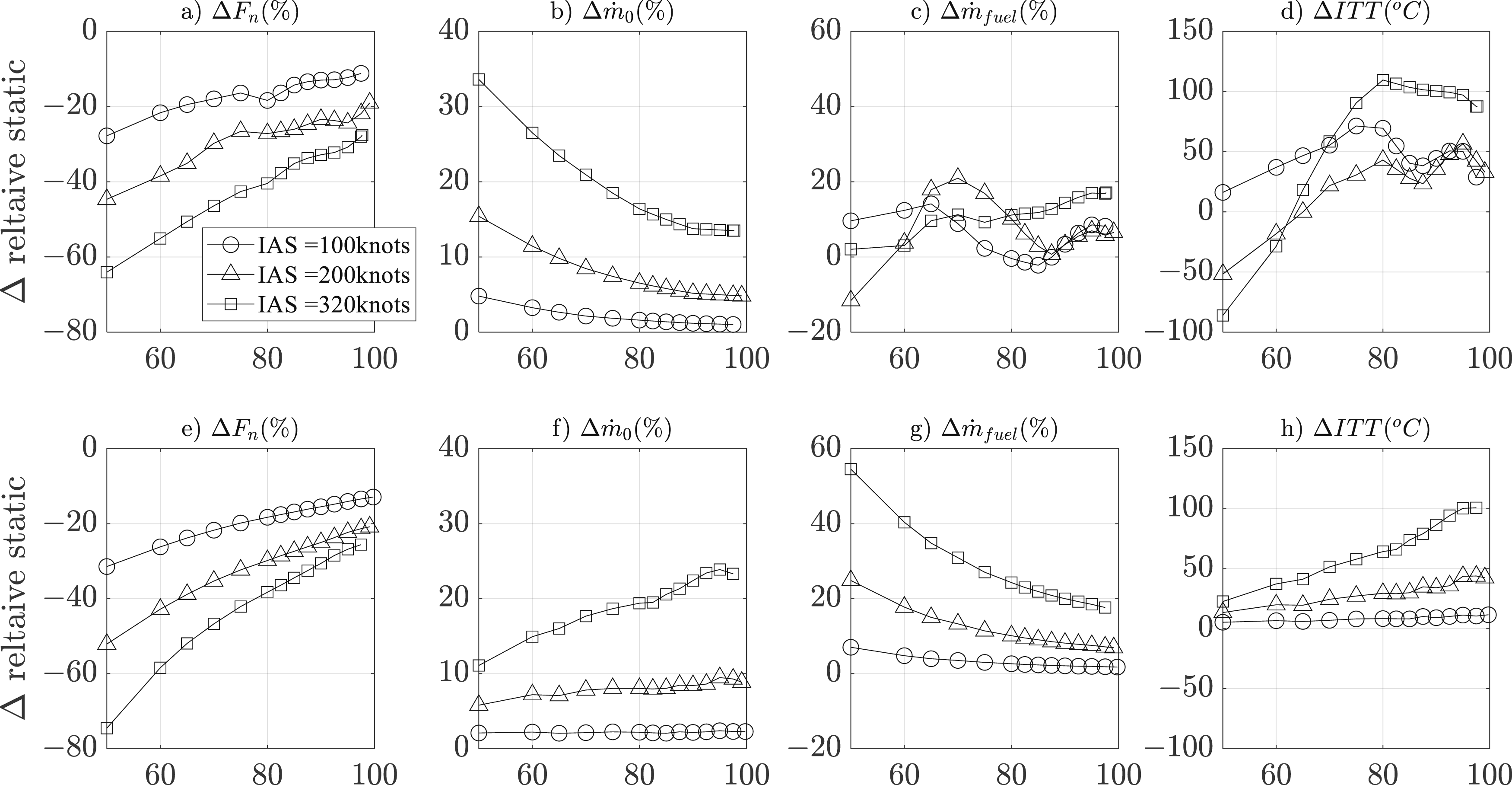
During the comparisons presented in the previous sub-section, suspicious ${\dot{m}}_{fuel}$ and $ITT$ data were detected in the VRESIM, which posed a concern about their quality and reliability. The data quality issue concerned an overlap in the ${\dot{m}}_{fuel}$ and $ITT$ curves when increasing flight velocity (or $MN$ ). At a constant ${NL}_{corr}$ , flying at higher $MN$ causes the thrust production to decrease, as the inlet flow linear momentum increases when higher flight speeds are achieved. Additionally, the total engine airflow is also expected to rise as a consequence of the bigger inlet flow momentum. The results presented in Figure 11 show the differences relative the static condition for the VRESIM (top row) and the CM-8C5B1-Base (bottom row). In Figure 11(a)–(f) the lines do not cross each other, as expected.

Figure 11.

Performance deviations relative to static conditions at sea-level. Top row a)−d): VRESIM, bottom row e)−h): CM-8C5B1-Base. The x-axes in a)−h) correspond to ${NL}_{corr}$ in %.

Another consequence of increasing $MN$ at constant ${NL}_{corr}$ is that the engine requires a higher fuel flow rate to maintain the aircraft speed, which in turn increases hot section temperatures, e.g., $ITT$ . This is true for the CM-8C5B1-Base (Figure 11(g) and (h)) but not for the VRESIM (Figure 11(c) and (d)). For the latter, an odd behavior in both ${\dot{m}}_{fuel}$ and $ITT$ signals was observed, i.e., the lines should not intersect. For example, in Figure 11(c), the lines overlap at ${NL}_{corr}$ = 90% for IAS = 100 and 200 knots. On the contrary, in Figure 11(g), for the same flight speeds and ${NL}_{corr}$ , the difference in fuel flow is + 6%, which points towards the expected direction.

The data quality observations discussed above caused concerns about the fuel flow errors between the CM-8C5B1-Base and the VRESIM, given that they are heavily influenced by the above-mentioned abnormal behavior. Therefore, a lower weighting factor ( $\lambda$ ) was used for fuel flow during the model match ( ${\lambda }_{{\dot{m}}_{fuel}}$ = 0.3 vs ${\lambda }_{F_n}$ = 0.7). The reason behind establishing these weighting factors was to achieve an appropriate balance between thrust matching and penalizing fuel flow, without overemphasizing either. A comparison of three different sets of weighting factors is presented in Figure 12. This figure shows the errors for each of the flight condition, as depicted in Table 1, using three pairs of weighting factors: ${\lambda }_1$ = (0,5,0.5), ${\lambda }_2$ = (0.9,0.1), ${\lambda }_3$ = (0.7,0.3). The rightmost column shows the results from the selected pair used in this research ( ${\lambda }_3$ ). The first pair ( ${\lambda }_1$ ) served as the reference set of errors for comparison with the other weighting factors. When using ${\lambda }_2$ , the thrust errors are significantly improved, but fuel flow presents a more pronounced scatter compared to ${\lambda }_1$ . Finally, ${\lambda }_3$ , was found to provide the right balance, with thrust showing a good match relative to the expected accuracy in this research, while fuel flow is slightly penalized, resulting in more scatter than thrust.

Figure 12.

Weighting factors sensitivity comparison.

Model match

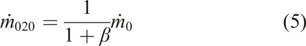
The model match involved, first, a revision of the Aerothermodynamic Design Point (ADP) assumptions. Second, a recalibration of both the fan map speed lines ( $\delta N_{120,corr}$ ) and of the adiabatic efficiency in the LPT map ( $\delta {\eta }_{LPT}$ ). The ADP assumptions remained fixed to those presented in Ref. 21 except for one parameter, the total engine airflow ( ${\dot{m}}_0$ ), which was revised based on the results presented previuously. In contrast to the other parameters assessed in this work (e.g., $F_n$ and ${\dot{m}}_{fuel}$ ), ${\dot{m}}_0$ is part of the set of assumptions that defines the ADP, and which are input to the engine cycle model for computing the nozzle areas and the maps’ scaling factors. The ${\dot{m}}_0$ was reduced by 4.07% to match that of the VRESIM (per Table 3). It is noteworthy that in Ref. 21, ${\dot{m}}_0$ was established based on both the fan face diameter and the $MN$ , i.e., 46.2 in (1.173 m) and 0.55, respectively. The latter was defined as an average of the range proposed in Ref. 41 i.e., $MN$ : 0.5-0.6. The revised ${\dot{m}}_0$ produced a fan face flow $MN$ = 0.505, which still lies within this $MN$ range. The revised ${\dot{m}}_0$ caused a reduction in the nozzles’ exhaust areas in both primary and secondary streams, ${\mathrm{\Delta }A}_{180}$ = −4.0% and ${\mathrm{\Delta }A}_{080}$ = −3.8%. Due to the proportionality of these $\mathrm{\Delta }A$ , the area ratio presented in Section 4 was not impacted ( $A_{180}/A_{080}$ = 3.9). Indeed, the magnitude and direction of these area changes are as expected. The flow areas are smaller because both primary and secondary stream flows are reduced by 4.07%; additionally, the bypass ratio remains fixed, $\beta$ = 5.0 ²¹ . The relationships between ${\dot{m}}_0$ and $\beta$ in the primary ( ${\dot{m}}_{020}$ ) and secondary flows ( ${\dot{m}}_{120}$ ) are presented in equations (5) and (6), respectively. From these equations it can be observed that, for a fixed $\beta$ , the flow through each stream solely depends on ${\dot{m}}_0$ . Additionally, equation (7) presents the relationship between flow area ( $A$ ), mass flow ( $\dot{m}$ ), Mass Flow Parameter ( $MFP$ ), total temperature ( $T_0$ ) and pressure ( $P_0$ ). For each nozzle exhaust, stations 080 and 180 in Figure 2, the $MFP$ , $T_0$ , and $P_0$ remain nearly constant between the original and revised ADP, thus, their respective $\mathrm{\Delta }A$ are driven by the corresponding $\mathrm{\Delta }\dot{m}$ .

${\dot{m}}_{020}=\frac{1}{1+\beta }{\dot{m}}_0$

(5)

${\dot{m}}_{120}=\frac{\beta }{1+\beta }{\dot{m}}_0$

(6)

$A=\frac{\dot{m}*\sqrt{T_0}}{P_0*MFP}$

(7)

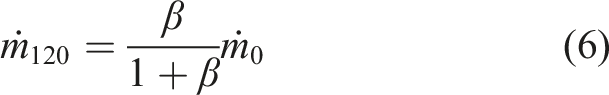
The adjustments to the cycle model ( $\delta N_{120,corr}$ and $\delta {\eta }_{LPT}$ ) are presented in Figure 13. These adjustments are a function of the power settings and the flight $MN$ . For $\delta N_{120,corr}$ (Figure 13(a)), the adjustments are larger for low $MN$ (0.182 and static) and tend to cluster in the same family. Conversely, they are smaller for high $MN$ (0.547 and 0.80), grouping in a different family. It is important to note that the shape of the curves is similar between the two $MN$ families. Based on these observations, one set of adjustments per family was created, one for $MN$ ≤ 0.182 and the other for $MN$ ≥ 0.547; when the $MN$ lies between these two, a 2D-linear interpolation was used to compute the adjustment. On the other hand, for $\delta {\eta }_{LPT}$ (Figure 13(b)), the adjustments for different $MN$ are close to each other for ${NL}_{corr}$ ≥ 85% and separate into two families below this threshold; these families correspond to the same $MN$ as for $\delta N_{120,corr}$ . In Figure 13, it is observed that both $\delta N_{120,corr}$ and $\delta {\eta }_{LPT}$ are relatively small for mid-to-high power (i.e., ${NL}_{corr}$ = 70% to 100%), however, these values become significantly large for lower power-settings, particularly for $\delta {\eta }_{LPT}$ . The derivatives $\frac{\partial F_n}{\partial {\eta }_{LPT}}$ and $\frac{\partial {\dot{m}}_{fuel}}{\partial {\eta }_{LPT}}$ , used during the matching process, become weak as the power-setting decreases; therefore, larger $\delta {\eta }_{LPT}$ are expected to minimize the errors between the cycle model and the VRESIM. The justification for these large adjustments is based on the simplified linear model described in the previous section. This linear model does not care if the actual cycle model can deal with such large adjustments in the turbomachinery maps, which are likely to cause convergence problems. Therefore, to avoid such problems, the large adjustments at low power-settings were restrained to a constant value for both $\delta N_{120,corr}$ and $\delta {\eta }_{LPT}$ ; in the case of $\delta N_{120,corr}$ , the restriction took place for ${NL}_{corr}$ ≤ 60%, whereas for $\delta {\eta }_{LPT}$ it applied for ${NL}_{corr}$ ≤ 70%.

Figure 13.

Cycle model match adjustments: (a) fan map speed adjustment and (b) LPT map efficiency adjustment.

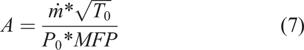
The comparison of the fan operating line and the LPT turbine efficiency for the CM-8C5B1-Base and the CM-8C5B1 are shown in Figure 14 for SLS and 35,000 ft (10,668 m)/ $MN$ = 0.80. The adjusted cycle CM-8C5B1 presents the expected changes. First, the fan operating line is increased (i.e., higher $\mathit{PR}$ at constant corrected flow) due to the $A_{180}$ reduction caused by the revised total airflow, which is only depicted in Figure 14(a) for 35,000 ft (10,668 m)/ $MN$ = 0.80 to avoid data overlap with the SLS. Second, the revised fan operating line is shifted towards the upper right, given that ${\delta N}_{120,corr}>$ 0 across power-settings (Figure 14(a)). The LPT adiabatic efficiency ( ${\eta }_{LPT}$ ) for the adjusted cycle is presented in Figure 14(b). For SLS, the proposed adjustment caused ${\eta }_{LPT}$ to change rapidly as the turbine corrected speed ( $N/\sqrt{T_0}$ ) is decreased. For 35,000 ft (10,668 m)/ $MN$ = 0.80, the change in efficiency is less steep and causes an overall flat efficiency trend than for SLS.

Figure 14.

CM-8C5B1-Base versus CM-8C5B1: (a) fan operating line; (b) LPT turbine efficiency versus corrected turbine rotational.

The normalized performance levels comparison between the CM-8C5B1 and the VRESIM is presented in Figure 15. These comparisons include two other conditions not presented in Figure 8, i.e., 10,000 ft (3048 m)/ $MN$ = 0.182 and 20,000 ft (6096 m)/ $MN$ = 0.547. The four flight conditions presented in Figure 15 correspond to those of the data match presented in Table 1. In the case of the normalized $SFC$ (Figure 15(c)), once more, the VREISM data showed some unexpected behaviour for 20,000 ft (6096 m)/ $MN$ = 0.547, i.e., the curve does not present an absolute minimum and thus is ever-decreasing.

Figure 15.

Normalized performance CM-8C5B1 versus VRESIM: (a) thrust; (b) fuel flow; (c) $SFC$ ; (d) airflow.

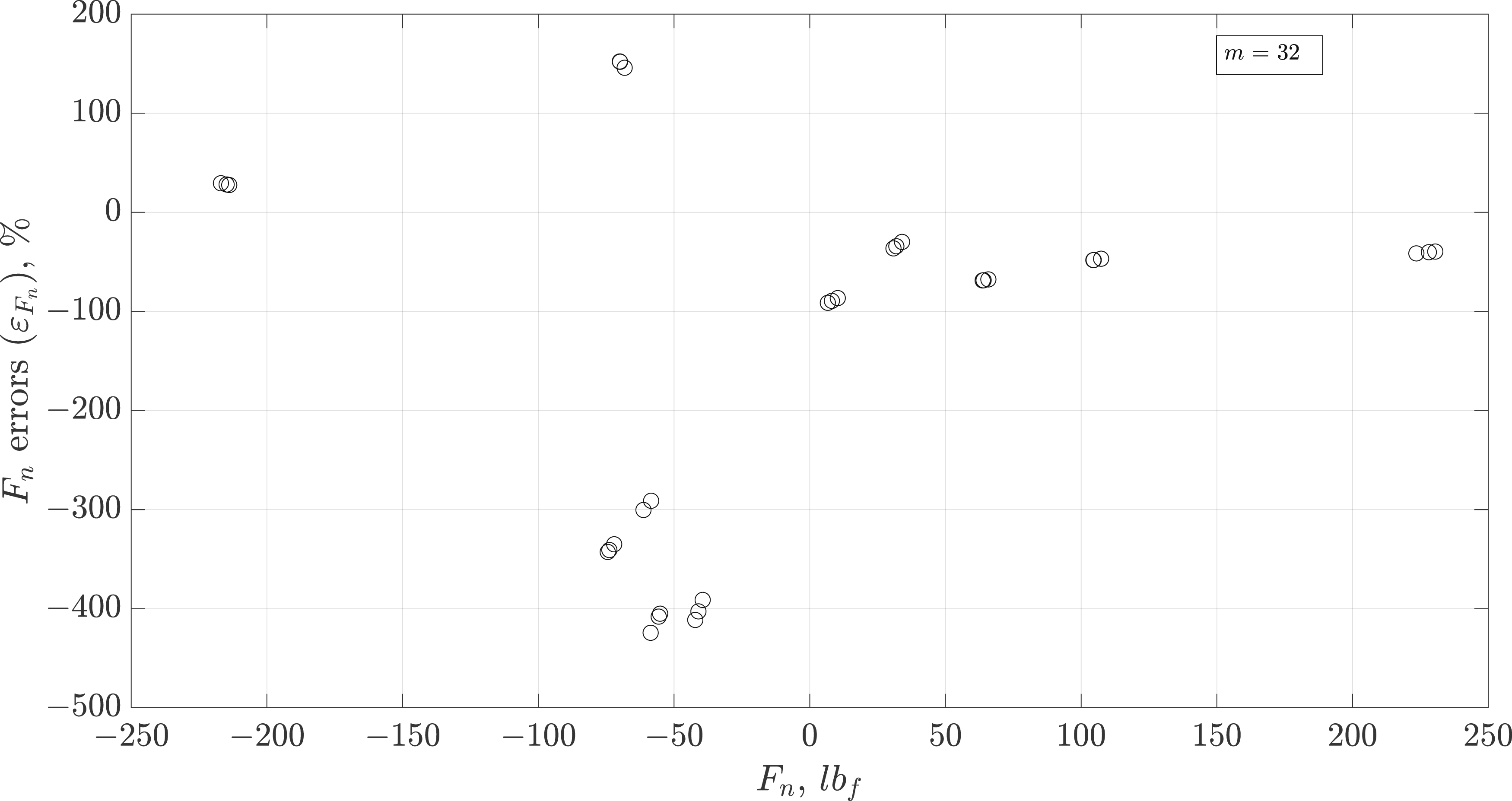
The full model validation for various flight conditions is presented in Figure 16. As in Figure 9, the histograms shown in Figure 16(c) and (d) encompass data for ${\epsilon }_{F_n}$ within ±25%. The accuracy of the matched model presented in Figure 16 is generally within the desired objective established in this research for both thrust and fuel flow. The improvement in model accuracy (CM-8C5B1-Base vs CM-8C5B1) is attributed to the reduction in individual averages and standard deviations (i.e., at constant ${NL}_{corr}$ ), as observed in Figure 17. In the CM-8C5B1 model, the individual averages tend to center around zero, whereas in the CM-8C5B1-Base model, these averages are biased toward negative values (see Figure 10). In Figure 17(b), the individual standard deviations for both $F_n$ and ${\dot{m}}_{fuel}$ are reduced overall, leading to an improvement in model accuracy. However, it is important to note that the accuracy target is not met at low power settings. The large thrust errors observed at these power settings are shown in Figure 18, which includes a sample of $m$ = 32 data points. These large errors correspond to small (both positive and negative) values of $F_n$ . The negative values are associated with flight idle, where the inlet flow’s linear momentum exceeds the gross thrust produced by both the primary and secondary nozzles. Indeed, matching small absolute quantities with the desired accuracy becomes a significant challenge. For instance, consider a point from Figure 18 where $F_n$ = +105 lbf (469.6 N); to meet the ±5% accuracy, the CM-8C5B1 model would need to predict thrust within ±5.25 lb_f (23.4 N). Achieving this level of accuracy may be overly ambitious under conditions such as idle power settings. While the desired accuracy target was not fully met at low power settings, we remain confident in the CM-8C5B1 response, as shown in Figure 15, where the model accurately reflects the expected trend of the absolute values throughout the entire power range.

Figure 16.

CM-8C5B1 versus VRESIM errors. (a) $F_n$ errors versus ${NL}_{corr}$ ; (b) ${\dot{m}}_{fuel}$ errors versus ${NL}_{corr}$ ; (c) $F_n$ errors histogram; (d) ${\dot{m}}_{fuel}$ errors histogram.

Figure 17.

(a) average ( $\mu$ ) and (b) standard deviation ( $\sigma$ ) errors (CM-8C5B1-Base and CM-8C5B1).

Figure 18.

Thrust ( $F_n$ ) errors at low power-settings.

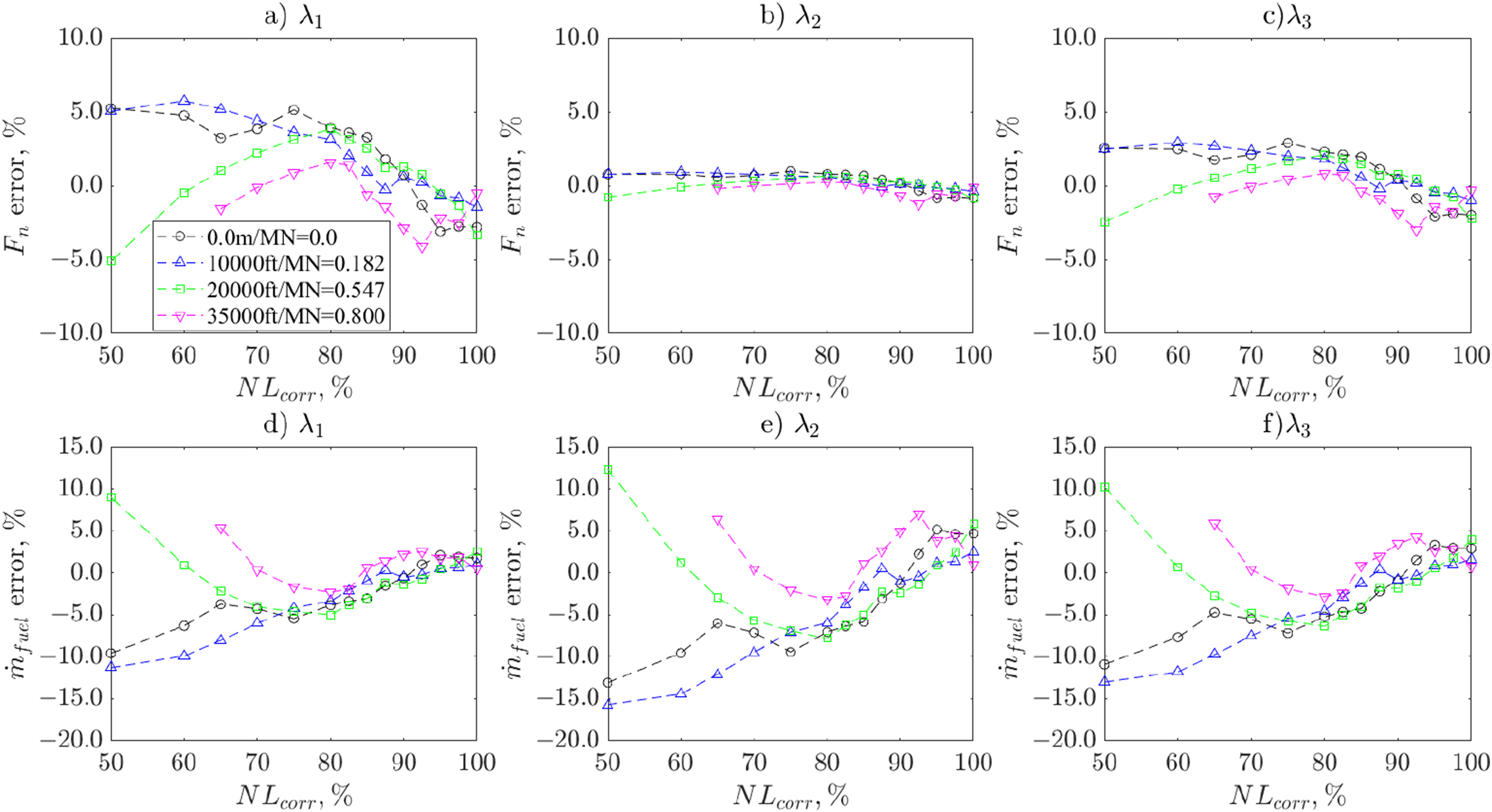
To further complement our discussion, the errors for ${\dot{m}}_0$ and $ITT$ are presented in Figure 19. As shown, the errors for ${\dot{m}}_0$ are overall within the desired accuracy. For $ITT$ , although no specific accuracy criterion was defined, it is observed from Figure 19(b) that the $ITT$ errors tend to revolve about zero for ${NL}_{corr}$ = 85%-100%. However, the scatter at constant ${NL}_{corr}$ was considered somewhat high. For example, within this range of ${NL}_{corr}$ , the standard deviation of $ITT$ $({\sigma }_{ITT}$ ) is approximately 20°C (36°F).

Figure 19.

CM-8C5B1 versus VRESIM errors. (a) ${\dot{m}}_0$ errors versus ${NL}_{corr}$ , (b) $ITT$ errors versus ${NL}_{corr}$ ; (c) ${\dot{m}}_0$ errors histogram, (d) $ITT$ errors histogram.

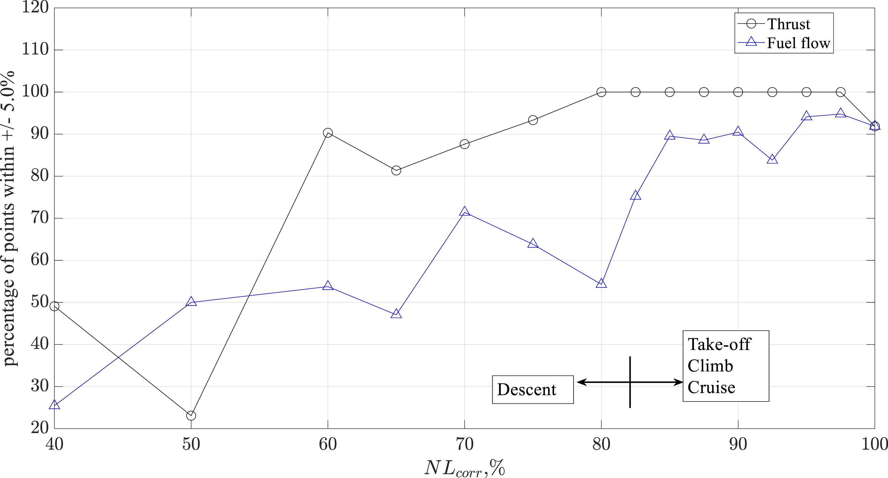
Finally, a further assessment of the model accuracy was performed based on future needs. The CM-8C5B1 is envisioned to simulate flight mission profiles in which the engine is driven at different power regimes (take-off, climb, cruise, idle). Given that the CM-8C5B1 performs consistently, independently of the flight conditions (altitude, $MN$ , temperature), the variable that most affects its accuracy is the power settings (i.e., ${NL}_{corr}$ ). Figure 20 shows the percentage of points that lie within the prescribed accuracy at each ${NL}_{corr}$ level. As it is observed, the $F_n$ accuracy was deemed adequate for ${NL}_{corr}$ = 75 to 100%, where at least 92% of the points fall within ±5.0%. This power setting range covers most parts of the mission regimes of interest: take-off, climb, and cruise in a typical CRJ-700 mission. Meanwhile, the ${\dot{m}}_{fuel}$ accuracy was deemed satisfactory for ${NL}_{corr}$ = 85% to 100%; overall, about 90% of the data points met the desired accuracy. The fuel flow accuracy declines below ${NL}_{corr}$ = 85%, primarily due to data quality concerns and the associated lower weighting factor applied during the model matching process.

Figure 20.

CM-8C5B1 accuracy across power-settings.

Complementary discussion

An important aspect of this research is that, while it focused on a specific engine model (CF34-8C5B1) based on the interests of our research group, the approach for performing data quality checks (e.g., data stability, repeatability) and the methodology for matching engine data can be applied to any other type of gas turbine engine data used in propulsion or power generation. This includes data from both analytical models (such as flight simulators) and experimental datasets. Additionally, we wish to continue advocating for the use of physics-based models, through which it is possible to make observations such as those presented in this study, specifically regarding the suspicious data originating from the flight simulator. It is important to emphasize that this capability cannot be replicated by other recently popular methods, which can only yield reasonable results once they have been trained. However, in order to be properly trained, such methods require reliable input data. Therefore, we believe that, when modeling the performance of gas turbines, the use of physics-based models is essential and should always be employed in parallel with other novel techniques under investigation.

Finally, some aspects for improvement in future research are briefly discussed. First, addressing the data quality issues observed in fuel flow and $ITT$ data obtained from the VRESIM is essential. However, this presents a challenge, as reliable alternative data sources, such as experimental data, are not readily available. Second, a more robust criterion for model accuracy at low power settings should be defined, potentially establishing an absolute level of accuracy rather than relying on percentages. Lastly, a significant avenue for future research lies in exploring alternative optimization methods. While the simplified performance model representation has proven effective in providing a simple, yet robust, solution to the matching model formulation, further studies should consider other optimization techniques (e.g., non-gradient-based methods). Of particular interest would be to assess whether such methods are more robust (i.e., avoid convergence issues), provide better match accuracy, and reduce computational costs.

Conclusions

This work established an accurate cycle model to represent the CF34-8C5B1 engine. The model accuracy was focused on the thrust and the fuel flow rate, which are of paramount importance to establish the $SFC$ . The baseline model (CM-8C5B1-Base), despite its overall low accuracy, provides reasonable predictions, especially at high power settings, considering that it has not been trained (or calibrated). These reasonable predictions are due to the fitness of the ADP assumptions, and the fidelity of the thermodynamic physics-based model used in this research. Moreover, the use of a physics-based model allows us to detect suspicious signals from the VRESIM engine model and take appropriate actions to mitigate their impact in the model match. It is very likely that such detection and mitigation cannot be thoroughly achieved with other sophisticated methods that do not rely on physics. The final matched model (CM-8C5B1) was deemed to meet the desired accuracy for the net thrust and fuel flow, particularly for establishing predictions across the power settings of interest in a CRJ-700 flight mission. Additionally, it also provided a good prediction for the total engine flow across the same power settings. For the $ITT$ , as with fuel flow, the accuracy is compromised due to the abnormal signal obtained from the VRESIM real-time engine model. An acceptable average $ITT$ match was generated for mid-to-high power settings, however, the scatter of the errors is rather high ( ${\sigma }_{ITT}$ = 20°C). To address the issues related to fuel flow and $ITT$ accuracies, alternative sources of information, such as experimental engine data, should be consulted for potential future research.