Sage Journals: Discover world-class research

Abstract

We develop a computational fluid dynamics (CFD) framework to design a feedback circulation control system to compensate for fluctuations in the fixed-wing aircraft caused by wind gusts. Circulation control actions are realized using dynamic boundary conditions in the CFD simulations. The dynamic flow responses with the circulation control are obtained by solving the unsteady Reynolds-averaged Navier-Stokes equations. The dynamic lift responses at several oscillation frequencies of wind gusts and the plenum chamber pressure, which controls the circulation, are also obtained. A system identification algorithm from control theory establishes the transfer functions corresponding to the frequency responses. Based on the transfer functions and the aerodynamic characteristics of circulation control, a feedback circulation control algorithm is designed. The performance of the feedback control system is verified by the CFD simulation coupled with the controller as time-varying boundary conditions. At each time step, the controller determines the parameters in the boundary condition according to the instantaneous lift calculated in the previous time step. The simulation results show that the circulation control effectively compensates for the lift perturbations caused by vertical directional wind gusts. The proposed unsteady CFD simulation frameworks provide high-fidelity evaluations of feedback control systems, and it will save costly efforts to set up unsteady wind-tunnel experiments.

Keywords

Circulation control gust alleviation unsteady aerodynamics closed-loop flow control CFD

Introduction

Circulation control is one of the active flow control techniques. It uses actuators to introduce energy into the surrounding flow of a wing to increase lift or reduce drag by changing the circulation. The circulation control wing with a tangential jet sheet on its circular trailing edge has been investigated extensively since the 1970s.^1–16 It is initially used as a high-lift device to dramatically increase the lift coefficient for short take-off and landing. The original circulation control wing used steady blowing for designed operational points. Over the last two decades, there has been growing interest in using the circulation as a control effector.^11,17–23 Compared to conventional aerodynamic surfaces, the circulation control wing has fewer moving parts but a much higher lift coefficient up to 8-9.²⁴

When the conventional control surface deflects, it displaces air, and the air around the control surface accelerates. The acceleration causes additional non-circulation lift and increases the hinge moment.²⁵ As the hinge moment increases as the flight velocity increase, the bandwidth of conventional control surfaces is further restricted because of the decreasing rotational speed of electro or hydrostatic actuators.²⁶ Circulation control does not have these limitations. Circulation control changes the lift coefficient by injecting a tangential jet sheet that moves the rear stagnation point downward, increasing circulation around the aerofoil. Unlike the existence of the hinge moment on the conventional control surface, circular control is expected to instantly reposition the aft stagnation point without resistance. The dynamic bandwidth of circulation control is potentially higher than the conventional mechanical flap. The rear stagnation point moves as soon as the nozzle pressure changes. Recent research has found applications in gust alleviation thanks to its high effectiveness and fast response in changing the lift of an aerofoil.^27–29 Among the applications, the flow control actuators are actively adjusted according to the flow disturbance to maintain a stable lift.²⁷

The circulation control for gust alleviation brings challenges to computational fluid dynamics (CFD) simulations. The conventional control surfaces such as ailerons, elevators or flaps, have well-defined low order mathematical models.³⁰ These models are used with the rigid-body dynamics of aircraft to design controllers to stabilize the aircraft dynamics.^26,30 While most aerodynamic simulations of circulation control consider steady-state and the main concerns are the lift augmentation for quasi-steady blowing conditions.^3,10,31

Investigations on the dynamic performance of circulation control are still rare. The Kussner functions provide analytical dynamic models of the aerofoil for conventional thin aerofoils encountering unsteady wind.^32,33 To the best of the authors’ knowledge, there is no validated dynamic mathematical model for circulation control actuators. Some researchers treat circulation control as a first-order or second-order black box model,^27,34 or simply assume that circulation control is a proportional component in the system.³⁵ This is valid only when designing a controller providing its robustness is sufficient to tolerate modelling uncertainties and the system is in the linear region.

The majority of existing research on closed-loop circulation controls and active flow control techniques uses experimental methods.^36–40 In wind tunnel tests, flapping vanes generate gusts,⁴¹ and it is challenging to produce representative wind gusts due to mechanical constraints. Similar difficulties exist in the in-flight tests to find such a wind field. Unsteady CFD simulations, e.g., Unsteady Reynolds-averaged Navier-Stokes (URANS) solver provide reasonably accurate time-dependence results.⁴² The progress of high-performance computers enables large scale unsteady CFD simulations.⁴³ It has been feasible to simulate the flow with control algorithms to investigate the closed-loop performance.²⁷

The time-marching progress in unsteady CFD solvers is equivalent to the sampling of a closed-loop system. The flow properties of all cells in the CFD simulations are obtained at each time step. Every state and output including lift, drag, moment, and velocity components are accessible. It provides a significant advantage for control synthesis and validation compared to low-order models or wind tunnel experiments.

We are to provide a new method for circulation control design and validation. We use an existing circulation control aerofoil⁴⁴ with a circular trailing edge and a tangential nozzle. In the following sections: firstly, the CFD simulations with dynamic boundary conditions are validated; secondly, frequency responses are obtained using unsteady CFD simulation; thirdly, a circulation controller is designed using the frequency responses; fourthly, the performance of the controller is validated in the closed-loop CFD simulations; finally the conclusions are presented.

Circulation control system & CFD validation

The simulation model

We adopt the General Aviation Circulation Control aerofoil⁴⁴ shown in Figure 1. The aerofoil is modified from the GAW-1 aerofoil, a low-speed 17% thick aerofoil, where its sharp trailing edge deforms into a circular Coanda surface. A backwards-facing nozzle located on the upper side of the circular surface. On the upstream of the jet exit, a chamber supplies high-pressure air to the convergent nozzle. The remaining aerofoil shape is the same as the GAW-1 aerofoil except for the modifications to the trailing edge.

Figure 1.

Modified General Aviation Circulation Control aerofoil with a circular Coanda surface, where the dashed line depicts the original GAW-1 aerofoil.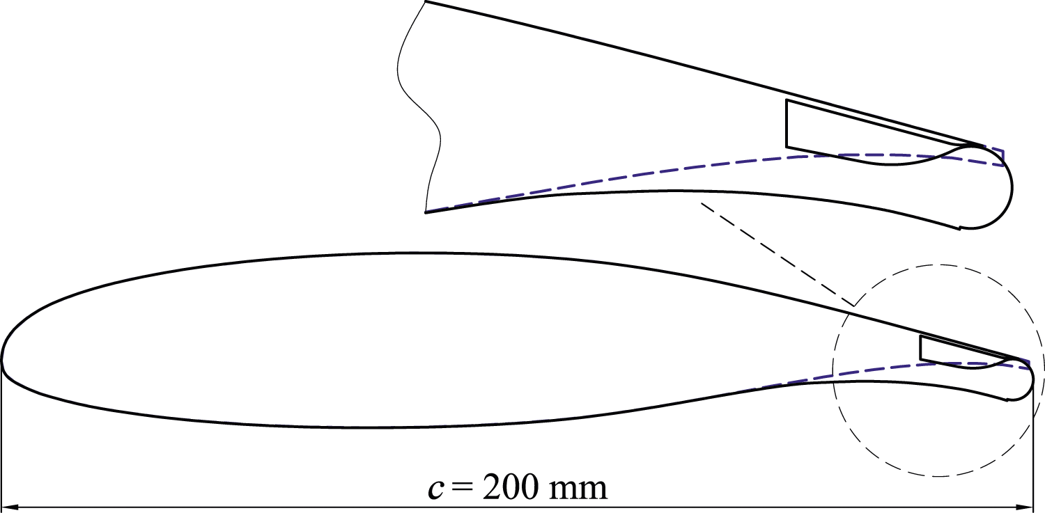

ANSYS ICEM is used to create the computational mesh shown in Figure 2. The mesh contains 149,001 cells in total. There are 510 points on the aerofoil surface and 210 points on the circular trailing edge. The thickness of the first layer next to the aerofoil is 10 μm given a wall y + value approximately equal to 1. The stagnation pressure in the plenum chamber of the nozzle determines the rear stagnation point and therefore alters lift. High-density meshes are placed around the trailing edge to accurately capture the jet’s separation.

Figure 2.

The mesh of the geometry.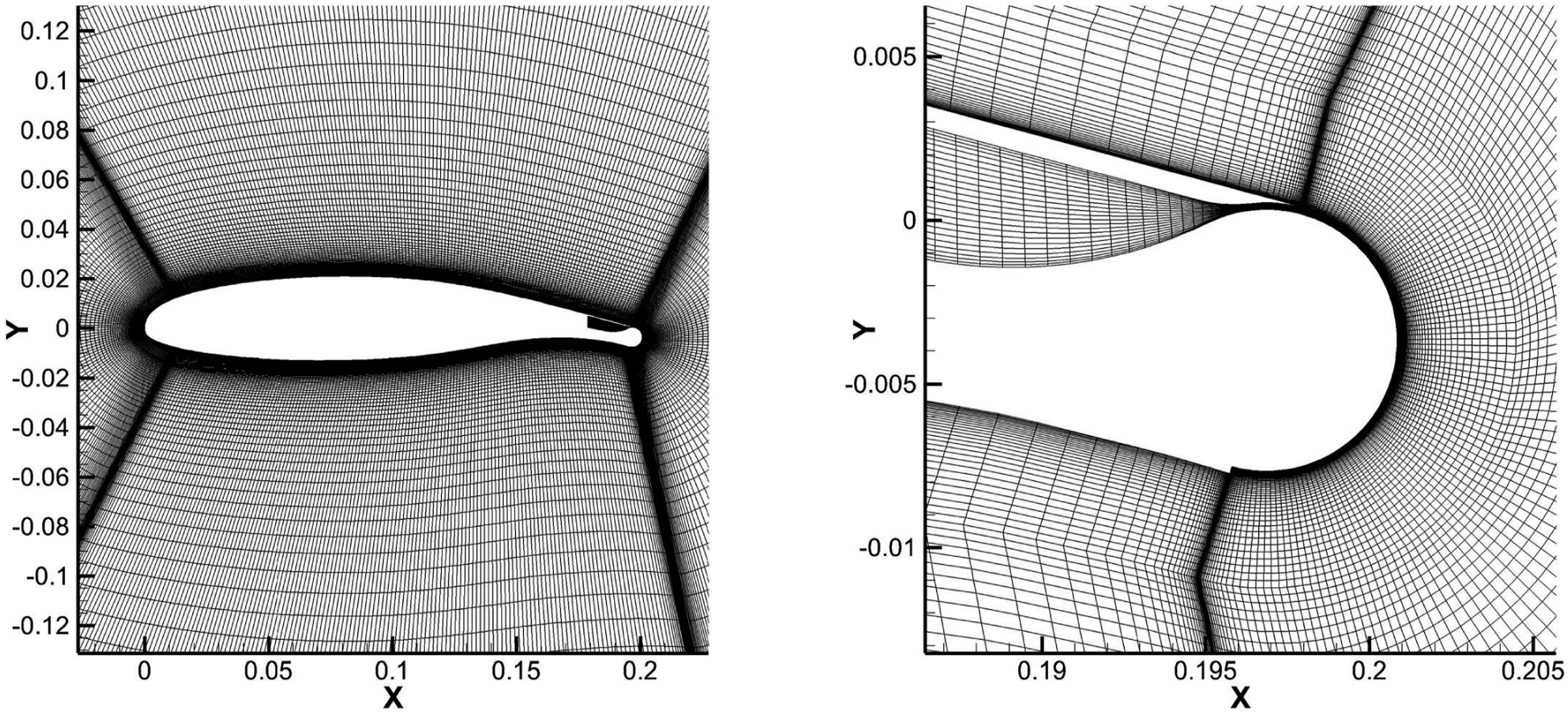

Figure 3 shows an example of the flow field around the trailing edge when the circulation control is activated. The nozzle exit is on top of the circular surface. A balance between centrifugal and radial forces causes the jet stream to attach to a circular surface. The jet stream then separates from the trailing edge in downstream due to the adverse pressure gradient. The circulation control aerofoil with blowing jet provides the functionality of an aerodynamic control surface, e.g., flaps. The jet controls the rear stagnation point and thereby controls the lift, corresponding to the deflection of a conventional flap. Jones et al.⁴⁴ have tested the design in the Basic Aerodynamics Research Tunnel in Langley Research Center and presented lift increments and surface pressure distributions for different angles of attack and nozzle pressure ratios.

Figure 3.

Boundary conditions of the nozzle (mm) and the velocity field at C_μ = 0.015.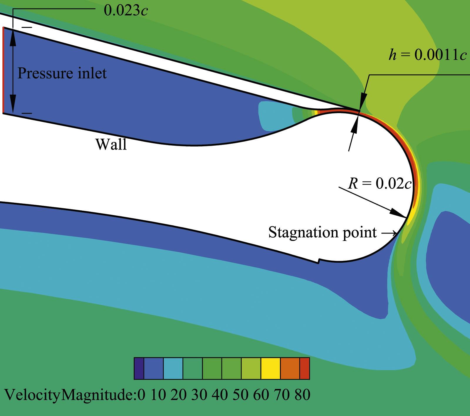

The lift augmentation due to circulation control depends on the rear stagnation point, where the upper and the lower streamlines meet. As the rear stagnation point moves downward, the streamlines around the aerofoil have higher curvatures and the lift coefficient increases. The exit velocity of the Coanda jet, which depends on the pressure of the plenum chamber, changes the location of the stagnation point. The chamber pressure and the lift change are the input and output of the control system. In practice, airdata sensors will be used to estimate the lift, whereas in this study, the lift is obtained by integrating the pressure distribution around the aerofoil calculated from the previous time step of the CFD solver.

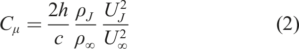
The momentum coefficient, C_μ, quantifying the blowing intensity is given by

C_{μ} = g (U_{J}) = \frac{2 h w}{c b} \frac{ρ_{J}}{ρ_{\infty}} \frac{U_{J}^{2}}{U_{\infty}^{2}}

(1)

where C_μ is considered as a function of U_J, i.e., g(U_J), h and w are the nozzle height and width, respectively, c is the chord length, b is the slot width or refers to the span of the wing, which is assumed to be equal to w, ρ_∞ and ρ_J are the densities of the free stream and the blowing jet, respectively, and U_∞ and U_J are the velocities of the free stream and the blowing jet, respectively.

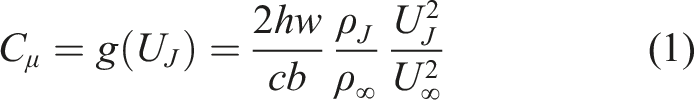
For a two dimensional simulation, w and b are removed, equation (1) is changed to the following form:

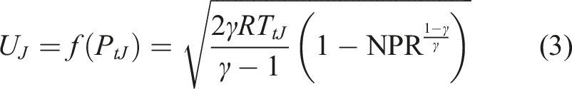
C_{μ} = \frac{2 h}{c} \frac{ρ_{J}}{ρ_{\infty}} \frac{U_{J}^{2}}{U_{\infty}^{2}}

(2)

The air from plenum chamber to the nozzle exit is an isentropic process.³ The mean jet exit velocity is determined by

U_{J} = f (P_{t J}) = \sqrt{\frac{2 γ R T_{t J}}{γ - 1} (1 - {NPR}^{\frac{1 - γ}{γ}})}

(3)

where U_J is considered as a function of P_tJ, i.e., f(P_tJ), γ is the heat capacity ratio, R is the gas constant, T is the static temperature, NPR is the nozzle pressure ratio equal to P_tJ/P_∞, P_tJ is the plenum stagnation pressure, and P_∞ is the exit static pressure.

As shown in Figure 3, the camber pressure, P_tJ, acts on the pressure inlet face. Compared to experiments, the boundary condition corresponds to the air supply system, e.g., air bleeding from the engine. Pneumatic proportional valves would adjust the control input, P_tJ. In CFD, it is realised by dynamically changing the boundary condition.

Steady validation

Few research uses the RANS method to study control problems, where the accuracy of time is vital. Currently, no validation case or database is available for such applications. This study uses multiple methods to assess the accuracy and reliability of the RANS approach in both steady and unsteady cases. Firstly the steady validation compares the CFD results with the wind tunnel results and verifies the accuracy of aerodynamic forces. Then the unsteady cases prove the accuracy of lift at different times. The validation cases increase the reliability of the closed-loop results.

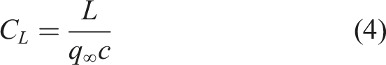
In steady-state conditions, the aerofoil lift coefficient, C_L, changes corresponding to P_tJ or C_μ have been simulated using steady CFD solvers and validated with experimental data by Jones et al.⁴⁴

The aerofoil lift coefficient is defined as:

C_{L} = \frac{L}{q_{\infty} c}

(4)

where L is the sectional lift force per unit span, q_∞ is the freestream dynamic pressure, c is the chord. Here C_L refers to the instantaneous lift acquired directly by the solver. Whereas for the dynamic boundary inputs, the C_Lss specifically refers to the lift acquired with a steady state, constant boundary condition and a constant freestream condition.

All CFD simulations are solved using the semi-implicit method for pressure linked equations (SIMPLE) and the Spalart-Allmaras (S-A) turbulence model with transient compressible solvers.⁴⁵ The spatial discretization method uses second-order finite volumes, and the temporal discretization uses second-order implicit methods for better time accuracy. The computational domain is initialized with the ideal-gas law in 288K at the sea-level International Standard Atmosphere (ISA) conditions. Figure 4 shows C_L in various C_μ inputs performed at a free stream velocity of 34 m/s, zero angles of attack (AoA). The CFD results generally agree with Englar’s experimental data.³

Figure 4.

Unsteady SA model C_L versus C_μ compared with experimental data at M = 0.1, AOA = 0°.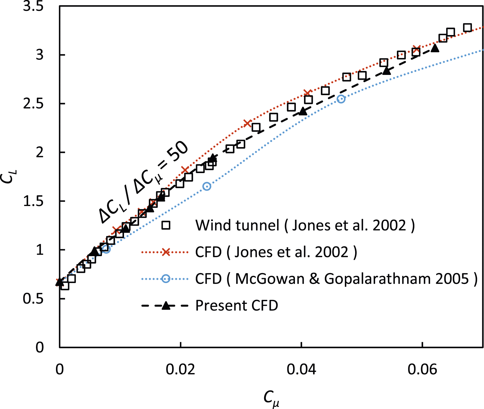

Figure 5 presents the pressure coefficient distribution over the aerofoil surface for C_μ = 0.06. The CFD data agrees well with the experiment on both the suction and pressure surfaces, including the peak suction value around the Coanda surface. It is identical to the CFD results conducted by Jones et al. who also used the S-A model.⁴⁴

Figure 5.

The wing surface distribution of pressure coefficient at C_μ = 0.06, compared with experimental data.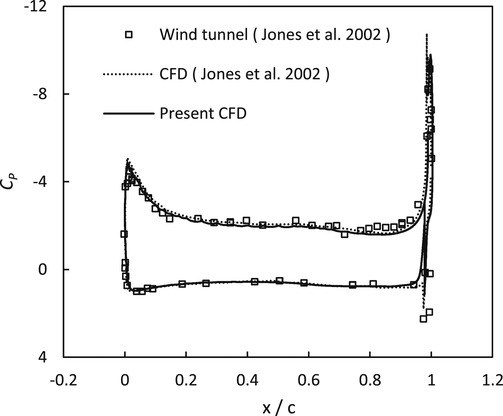

Figure 6 shows the variation of C_L with AoA for four different momentum coefficients. The present CFD is in very good agreement with the experiment, the maximum deviation appears at C_μ = 0.025, AoA = 6°, which is 0.14 lower than the wind tunnel C_L and it is acceptable. All CFD results are identical for C_μ = 0, indicating good agreement for the unblown cases. Note both of the reference CFD simulations used the S-A model. However, the CFD conducted by McGowan predicts 15% lower C_L for C_μ = 0.025 which is worse than the present CFD.

Figure 6.

C_L versus AOA in different blowing momentum coefficient at M = 0.1. Compared with experimental data.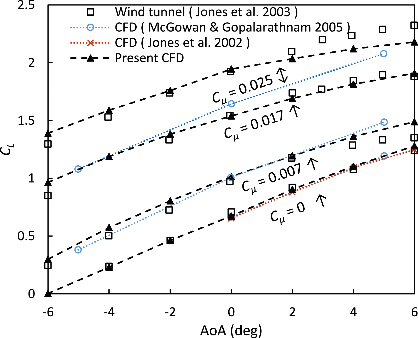

Unsteady validation

For the purpose of analysing dynamic performance, one of the gust models that has been widely used is the sharp edge gust.^46–49 Assuming an aircraft that is initially flying in a quasi-steady state in calm air, encounters a uniform vertical gust with a velocity of w_g, the interface between the calm air region and the gust region is a step change in velocity. Although an ideal sharp edge gust is not realizable in actual flight or in a wind tunnel, it can be studied by analytical methods or CFD simulations to understand the time history of incremental lift after it encounters a gust. Analytical solutions for this lift response to a sharp edge gust have been derived by Küssner,^32,33 and are used here to validate the unsteady CFD simulations. Küssner developed an exponential equation for a flat plate experiencing a unit step gust in an incompressible flow given by

Ψ (s) = 1 - 0.5 e^{- 0.13 s} - 0.5 e^{- s}

(5)

where Ψ(s) is the lift variation with non-dimensional distance travelled, s = (2Ut)/c, over the time period t. Note that the coefficients may have been modified in other references 50–52. We adopt the coefficients approximated by Sears et al.⁵³ The function was extended from a theory of non-uniform motion of a thin aerofoil in potential flow initially given in³³.

Although the Küssner function is derived for a thin flat plate, a thin symmetrical aerofoil should also give similar results.⁵⁴ A NACA0’]012 aerofoil was selected for the unsteady validation with a unit chord. Figure 7 shows the structured mesh generated using the Pointwise software, which has 807,000 cells with a circular-shaped domain dimensioned so that the far field boundary is approximately 10c from the aerofoil. There are 808 points around the aerofoil and 1001 points in the wall normal direction. The thickness of each mesh layer is gradually increased from 1 × 10⁻⁵m at the aerofoil surface, to 0.01 m in the free stream region. Beyond this, the edge length is kept uniform to ensure a relatively fine mesh in the freestream flow to reduce the numerical dissipation of the gust front. As a result, the free stream mesh is so dense and evenly distributed, that the mesh is not distinguishable in Figure 7 (left). The figure in the right is magnified one of the areas of interest. The final mesh has a wall y⁺ value less than 0.7.

Figure 7.

The computational mesh for unsteady validation of NACA0012 aerofoil, left: the computational domain with a uniform density from the aerofoil to the far field, right: the mesh distribution near the wall.⁵⁵

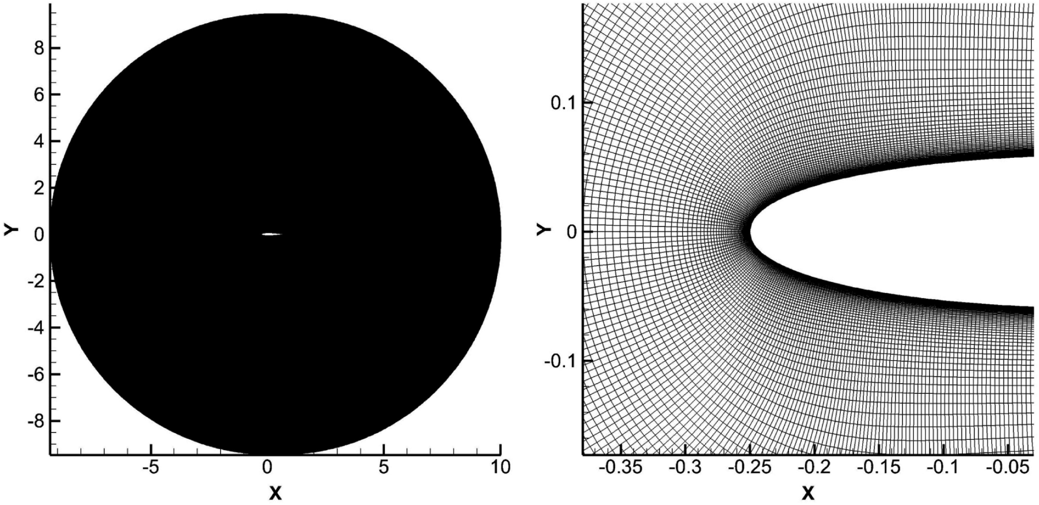
Although the previous GACC aerofoil was meshed using ICEM software, the mesh for the NACA0012 aerofoil was generated by Hyperbolic Extrusion using Pointwise software. In this approach, a marching front could be extruded from the wing surface to the far field. Despite the non-uniform distribution of points on the aerofoil surface, the Hyperbolic Extrusion method produces a high quality orthogonal mesh, and a smooth transition from a high to low density region to capture the propagating front, and avoids high aspect ratio cells near the far field, relative to the previous mesh strategy using ICEM (since the block topology used in ICEM is more suited for complex geometries). For both cases, similar parameters (including first layer thickness, growth rates and algorithm, and point distribution over the aerofoil surface) were used for the near wall region in order to achieve consistency between the two mesh approaches.A sharp edge gust is realized by applying an initial vertical velocity component to every cell in a specific field ahead of the aerofoil,^42,56,57 or by imposing an unsteady gust profile on the inflow boundary.⁵⁴ 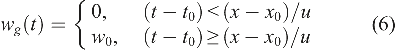The first method may cause convergence issues due to the discontinuity at the interface and is not available in most solvers. The second method is easily realizable but the gust front may be smeared due to numerical dissipation as the gust front travels from the inflow boundary to the leading edge of the aerofoil. In this study, the latter approach was used, with a high mesh density upstream of the aerofoil to reduce numerical dissipation and a user-defined function (UDF) that specifies a vertical gust front at the inflow boundary. Since this boundary has a circular shape, the gust front passes each element on the boundary at a different time, determined by the UDF. Thus, assuming x is the cell centre on the x-axis, the vertical velocity component of each face on the boundary is controlled using the function;

w_{g} (t) = {\begin{cases} 0, & (t - t_{0}) < (x - x_{0}) / u \\ w_{0}, & (t - t_{0}) \geq (x - x_{0}) / u \end{cases}

(6)

where x₀ is the initial position of the gust front which is on the far left end of the computational domain, t₀ is the time when the gust starts moving, w₀ is the vertical component of the gust velocity, u is the free stream velocity. This function describes when the gust front passes each face on the far field. Figure 8 displays an instantaneous vertical velocity distribution that clearly shows the gust front located at x = −5.5 m, as it travels from left to right. On the left side, a uniform vertical gust velocity w_g = 1 m/s is applied, whilst on the right side, the vertical velocity is zero. The direction of w_g is the same as the Y axis. Note the marching of the gust front is not enabled by any function, it automatically travels due to the freestream velocity.

Figure 8.

The vertical velocity field (m/s) showing the gust front marching from the left side of the domain.⁵⁵

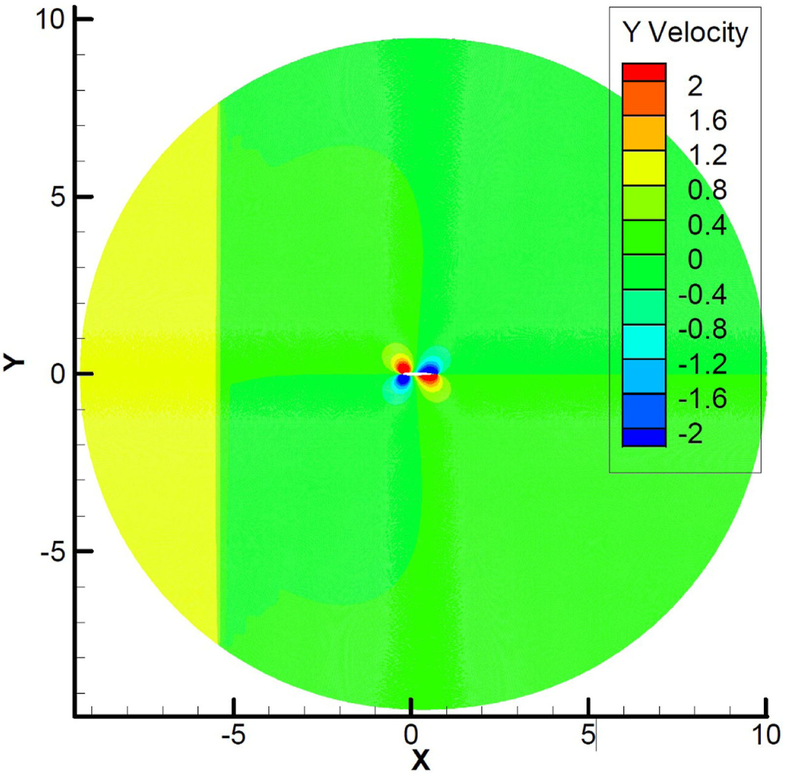
Simulations were performed for two streamwise velocities, U_∞ = 34 m/s (M_∞ = 0.1) and U_∞ = 68 m/s (M_∞ = 0.2), giving a chord Reynolds number, Re = 2.31 × 10⁶ and 4.62 × 10⁶ respectively. At t = 0, the initial position of the gust front is x = −10m. The penetration speed of the gust is the same as the free stream velocity, U_∞.

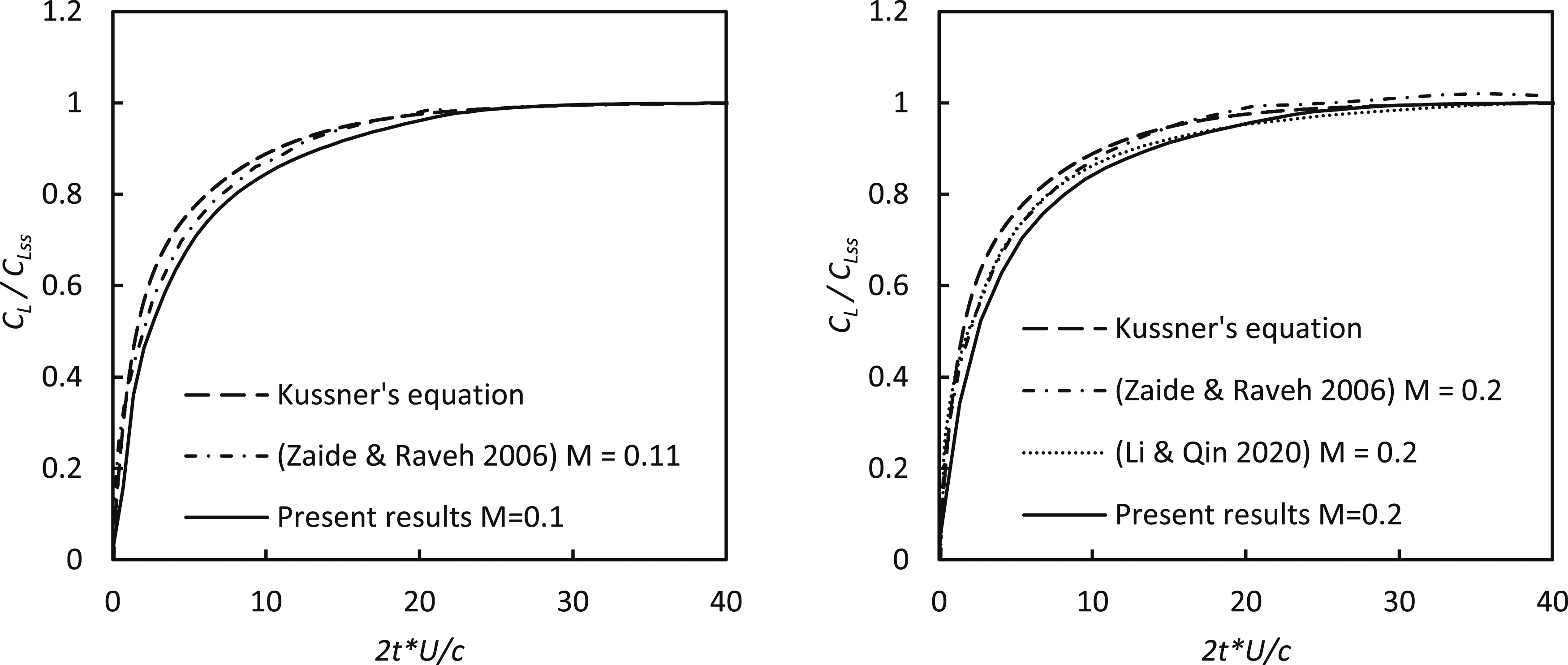
Unsteady simulations were initialised from a fully converged simulation with steady boundary conditions (U_∞ = 34 m/s or U_∞ = 68 m/s, AoA = 0°, T = 288K), prior to the UDF being used to create the gust front. As the gust front passes the aerofoil, a time history of C_L is recorded and compared with analytical results. Figure 9 gives the unsteady validation results for both M_∞ = 0.1 and M_∞ = 0.2 cases. Simulated results are in very good agreement with analytical solutions as well as simulated results from other researchers. There is a small lag compared with the analytical curve due to numerical dissipation. Considering two adjacent cells in the flow domain, since the velocity components are defined at the centroid, the discretization scheme will create a gradient over the distance between the two centroids, so a perfectly sharp edge is not achievable except for some custom codes.⁴² Consequently, it is difficult to determine the exact time when the gust front arrives at the leading edge, and it is assumed to correspond to the time when C_L increases to 5% above the steady state value, leading to a small inaccuracy in the interaction time and the lag that was observed compared with analytical results.

Figure 9.

Unsteady validation results of the NACA0012 aerofoil encountered a sharp edge gust, left: M_∞ = 0.1, right: M_∞ = 0.2.⁵⁵

Frequency response of circulation control system

We investigate the response, C_L, to the dynamic inputs, P_tJ, in a range of frequencies. The frequency response provides the data to establish an input-output model of the circulation control aerofoil, and the model is later used to design a feedback controller. After the controller is designed, the effectiveness of the controller is verified in CFD simulations using the URANS equations.

Typically, the dynamic characteristics of mechanical control surfaces are obtained in wind tunnel tests. As we focus on the unsteady aerofoil behaviour during vertical gusts, understanding the dynamic characteristics of the circulation control is essential to developing a control system. CFD simulations provide the lift response, where a periodic boundary condition varies the chamber inlet pressure. The time-step settings in the transient solver ensure to provide a time-accurate solution. We perform time-step independence verification for 10 Hz sinusoidal plenum chamber stagnation pressures in the 0-20 kPa gauge pressure range, provided 10 iterations per time step which gives converged solution in each time step.

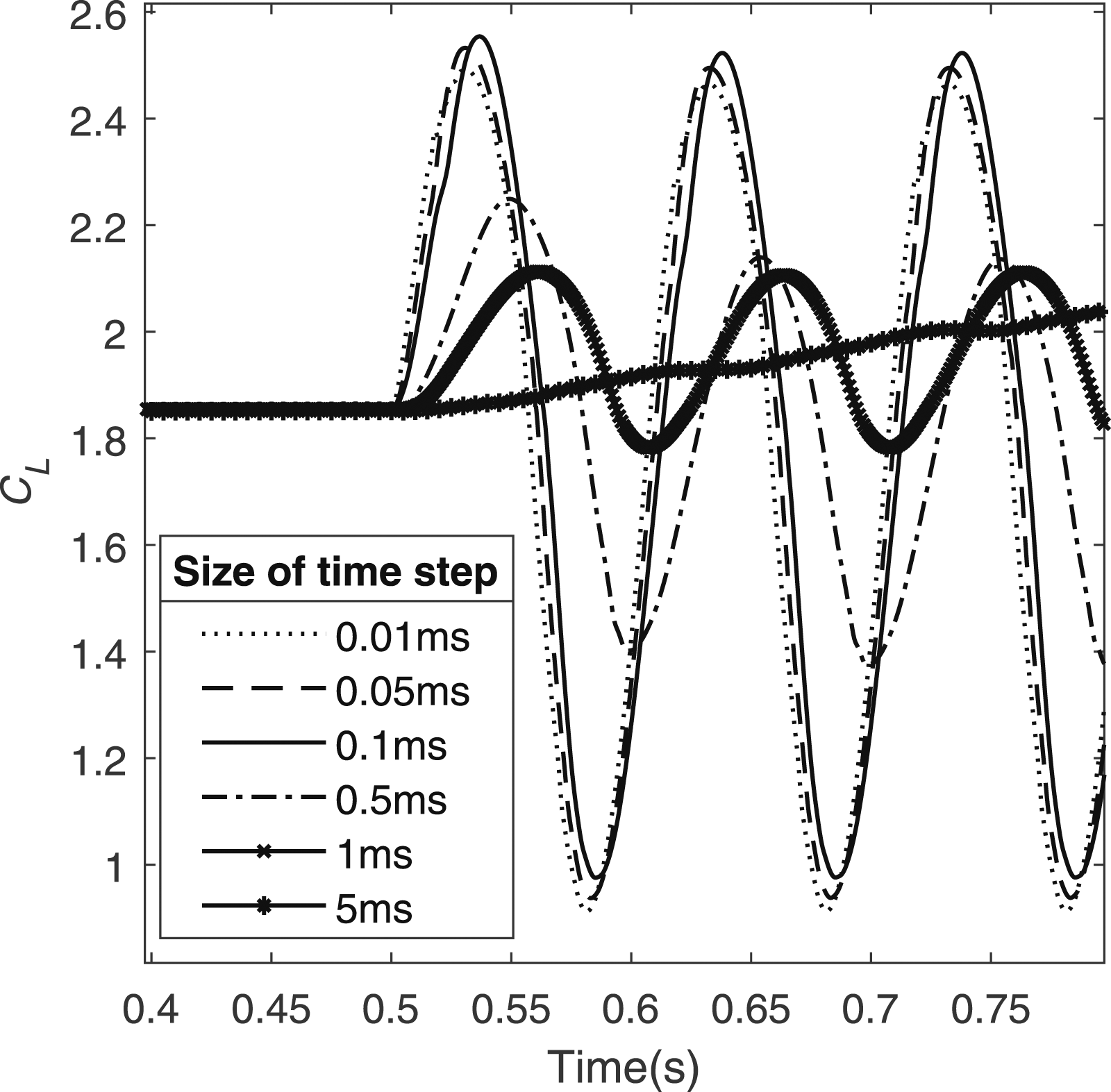
Figure 10 shows the C_L response for time steps from 5 ms to 0.01 ms with the periodic NPR starting after a steady simulation for the first 0.5s of the simulations. The lift responses for the time-step less than 0.1 ms are independent of the time step with some tolerances. The time-step, 0.1 ms, is used for all further calculations. The simulation for 12s requires about 22 h of elapsed computing time on the High-Performance Computer with 8 CPU (Central Processing Unit) cores. The response sampling frequency, 10 kHz, is much higher than the maximum input frequency, 50 Hz.

Figure 10.

Lift coefficient response in different time steps.⁵⁵

The dynamic lift response includes the actuator and the fluid response. For a conventional aileron actuated by hydraulic or electrical power, the actuation time contributes significantly to the overall time lag, whilst the flow response time is relatively small.⁵⁸ On the other hand, the pneumatic valve switching time used in circulation control is faster than the flow response time. The flow response is the time length for the rear stagnation location to settle. A typical high-speed pneumatic valve switches 1200 times per second.⁵⁹ The dynamic characteristics of circulation control mainly depend on the responses of surrounding fluid.^32,58

We perform CFD simulations for different input frequencies of the plenum stagnation pressure and obtain the magnitudes of the lift. Because of the unit differences, we choose to compare the relative magnitude of C_L to the steady-state lift coefficient, $C_{L_{s s}}$ . It provides an intuitive comparison of how the magnitude of C_L changes with the different frequency inputs. $C_{L_{s s}}$ is obtained by simulation with steady, continuous blowing. Given a particular input C_μ or P_tJ, the lift result $C_{L_{s s}}$ is determined. However, for an unsteady input, the output C_L can not be determined by the transient input value. It varies to the input frequencies due to the hysteresis of the fluid and the response of the surrounding flow pattern. At a high frequency (e.g. 10 Hz to 100 Hz), the lift no longer follows the input signal, and the amplitude of the output C_L decays. There is also a time lag between the input signal and the output signal. Figure 11 is a schematic of the desired C_L and the actual C_L. If the lift responds immediately to any frequency of C_μ, the lift should equal to the corresponding steady state value C_Lss at any time, as shown by the ‘Target C_Lss’ curve. The degradation of output can be quantified by the magnitude decay and the phase lag. The former is the ratio between the magnitude of C_Lss and the actual (measured) C_L, expressed in logarithmic scale by the convention in signal processing. The latter is the time lag between the two signals, expressed by the phase of the sinusoidal signal, assuming the frequency is ω. A large time lag deteriorates the controller’s performance.

Figure 11.

Response of lift to a sinusoidal input.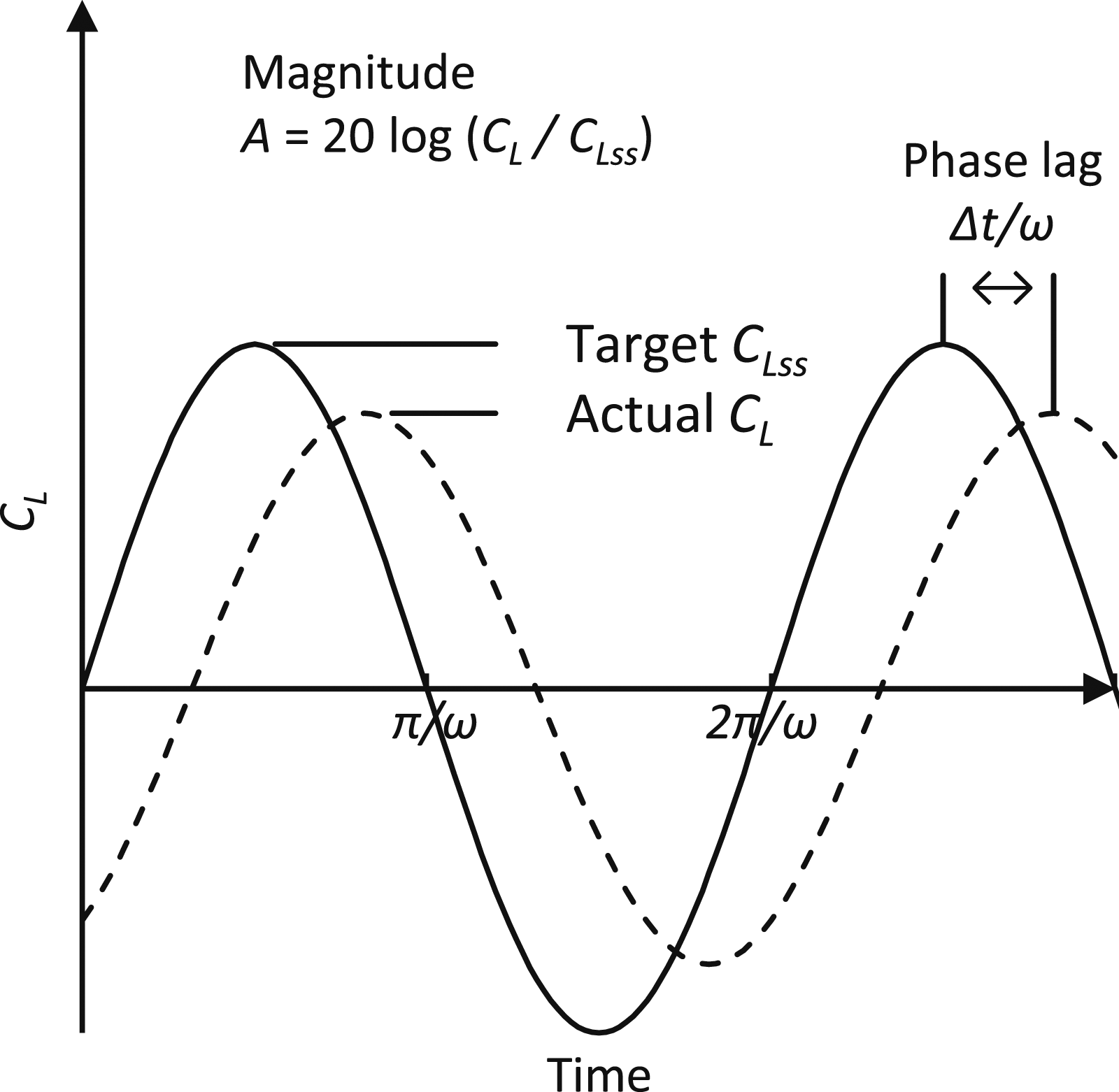

The following equation calculates the steady-state lift coefficient:

C_{L_{s s}} = h (C_{μ}) = h {g [f (P_{t J})]}

(7)

where h(C_μ) is the steady-state lift response to different nozzle pressure given by Figure 4. The relation between C_μ and P_tJ have both steady and unsteady terms. The ‘f()’ refers to the steady state relation, where a specified P_tJ gives a certain C_μ. It also has an unsteady effect with high-frequency periodical blowing, if P_tJ is dynamically changing in a high frequency, C_μ (also C_L) can not follow the variation of the input. The ‘g()’ function depicts the unsteady behaviour.

C_μ is calculated with jet velocity U_J which is affected by the low pressure region immediately behind the exit, this low pressure region is caused by the high curvature flow pattern and can not be determined before the simulation. Hence it is not possible to implement the dynamic changes of C_μ in the CFD simulations because U_J can not directly specified. On the other hand, the P_tJ change can be realized as a boundary condition of the nozzle wall. Hence, we treat P_tJ as the control input signal.

Figure 12 shows the Bode diagram of the dynamic CFD simulation results, where the frequency ranges from 0.5 to 50 Hz, the input amplitudes of ± 1 kPa or ±10 kPa, and the freestream Mach numbers, 0.1 or 0.2. For M = 0.1, the sinusoidal pressure with ±10 kPa variation has faster response and less decay in magnitude than the ±1 kPa curve. In addition, the M = 0.2 curve has less decay than the M = 0.1. As the lift response is from the surrounding fluid due to changing aerofoil boundary, intuitively, a high freestream velocity and/or high-pressure input results in a large magnitude response with a small phase lag. The overall bode plot shows that circulation control can be considered a linear first-order system for a fixed freestream velocity and input pressure magnitude.

Figure 12.

Comparison of Magnitude and Phase response with different nozzle pressure range and velocity.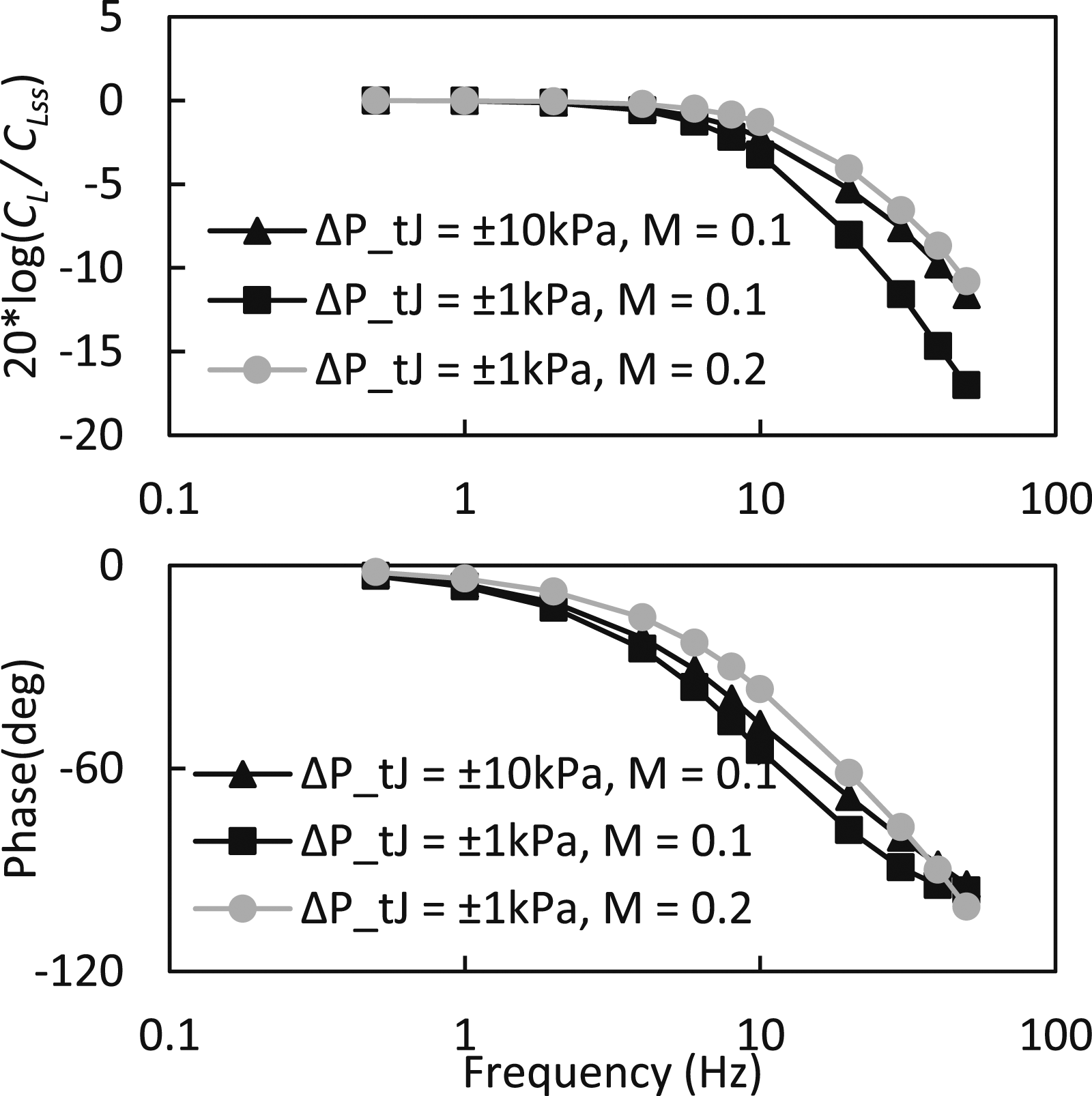

To design a feedback control algorithm, it is also crucial to identify the lift response to wind gusts. The CFD performs unsteady simulations with a constant P_tJ = 10 kPa. Time-varying axial gusts in the X direction are implemented in the CFD simulations. A dynamic freestream condition is applied on the far field. The Mach number varies between 0.09 and 0.11 periodically, with a frequency range from 0.5 Hz to 10 Hz. Time-varying vertical gusts are also implemented from the far field with a velocity range from 0 to 6.8 m/s and a frequency range from 0.5 to 10 Hz. The periodic velocity is created by a sinusoidal wave. Finally, the instantaneous C_L results are divided by the steady-state C_Lss with a constant boundary condition (M = 0.1), to compare the magnitude decay and the phase shift in different frequencies.

Figure 13 shows the Bode diagram for axial and vertical wind gusts. The magnitude for axial gust does not change significantly with higher frequencies compared to vertical gust, which is the case in a similar experimental study by Kerstens.²⁹ The lift responses to the axial and the vertical wind gusts, have the natural frequency at around 4 Hz and 6 Hz, respectively. This ‘natural frequency’ is purely the characteristic of the surrounding flow, it is not related to the structural frequency, only affected by the geometry of the aerofoil.

Figure 13.

Lift response to axial gust, P_tJ = 10 kPa, M = 0.1, ΔU_g = ±3.4 m/s, ΔV_g = 6.8 m/s.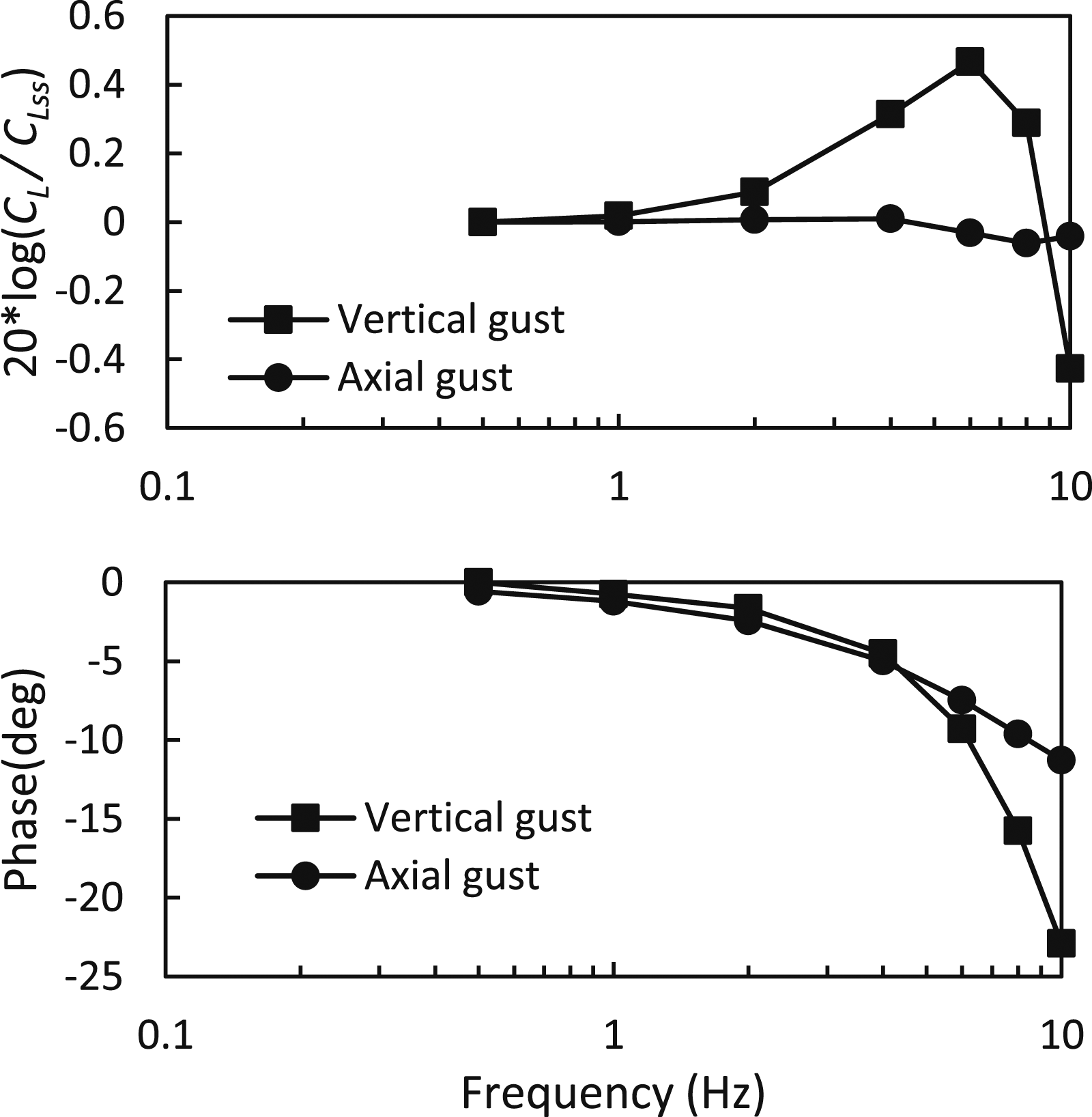

The aerofoil pressure distributions with sinusoidal P_tJ inputs resolved by CFD are listed in Figure 14. The C_p curves are snapshots at the moment when P_tJ reaches the peak (P_tJ = 11 kPa or 20 kPa) and valley (P_tJ = 9 kPa or 0 kPa) values. The pressure distributions under 0.5 Hz, 10 Hz, 50 Hz are shown, with two different input fluctuations, ±1 kPa and ±10 kPa respectively. As the sinusoidal frequency increases, the C_p curves are less responsive under a higher frequency, and the C_p curves with peak and valley P_tJ values are closer, the trend agrees with the magnitude plot in Figure 12. It indicates that the surrounding fluid can not follow the input instantly. For P_tJ = 0 kPa/20 kPa at 50 Hz, the two C_p curves are closer at the leading edge compared to the trailing edge. This is because the fluid near the leading edge reacts slower due to the longer distance to the nozzle exit.

Figure 14.

The aerofoil pressure distribution under different frequencies, M_∞ = 0.1.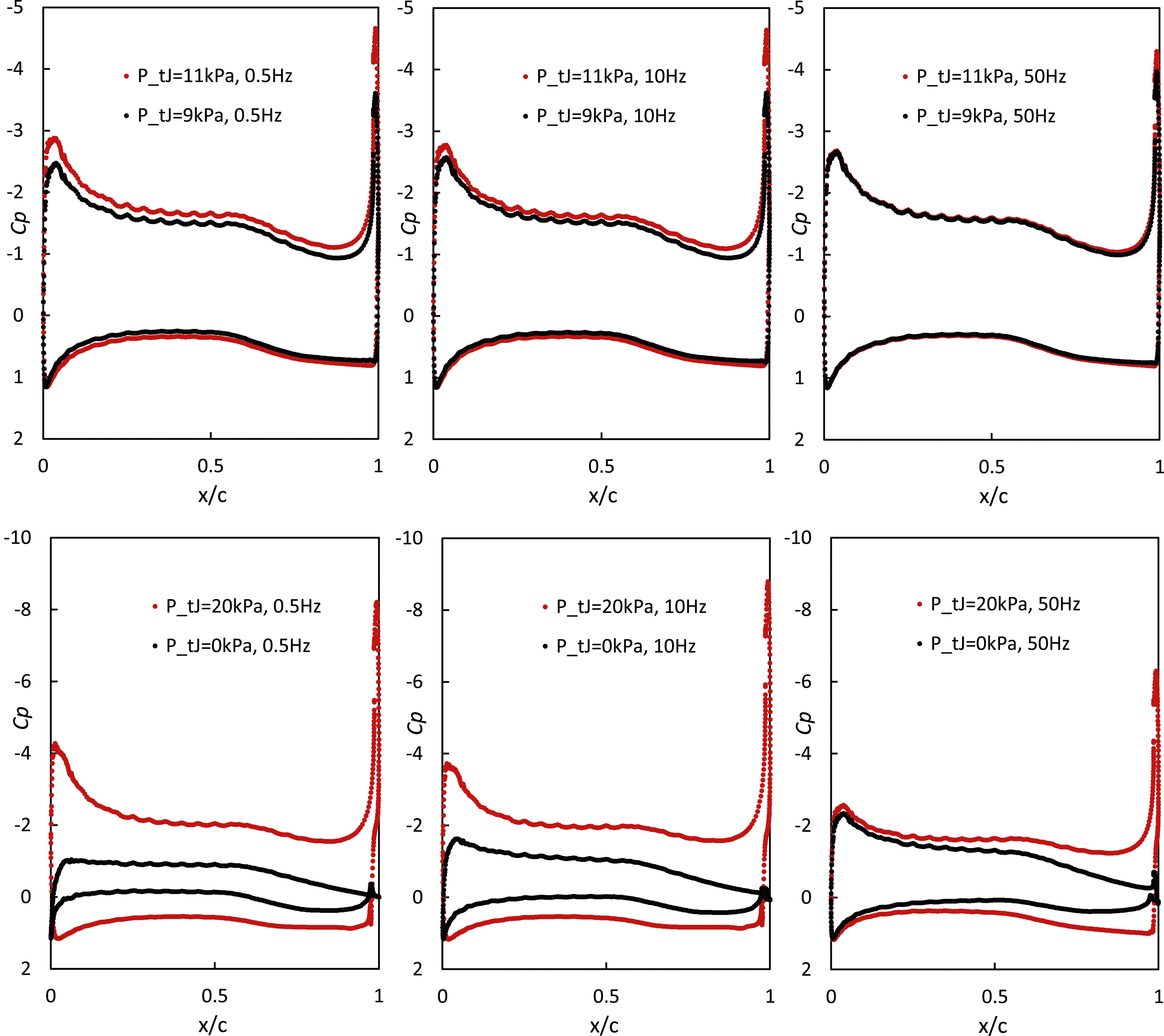

The corresponding flow field of the data frames shown in Figure 14 are plotted in Figures 15 and 16. The colour map shows the velocity magnitude normalised by freestream velocity U_∞ = 34 m/s (M_∞ = 0.1). The jet sheet wraps around the circular surface and accelerates the flow above the nozzle, leading to a rear suction peak in the C_p curves. The jet also creates a large separated wake near the circular Coanda surface. The rear stagnation point (separation point) is marked in each figure, and the separation angle θ refers to the circular angle relative to the nozzle exit. When P_tJ varies between 9 kPa to 11 kPa, the stagnation point changes between 98° and 111°, and the range reduces with higher frequency due to the flow hysteresis. The peak velocity at the nozzle exit is 148 m/s, then it gradually slows down and the jet sheet thickens downstream. The local velocity of the jet is close to U_∞ after it detached from the tailing edge. In comparison, when P_tJ varies between 0 kPa to 20 kPa, as shown in Figure 16. The stagnation point moves to θ = 180° at maximum P_tJ and is fully attached to the semi-circular surface. Similarly, as the frequency increases, the range of θ reduces to 66° − 142° at 50 Hz. The maximum U_J is 193.5 m/s at the nozzle exit. Although a pressure-based solver is used in the simulation, the Ansys Fluent solver has extended the application of pressure-based methods, the energy equations can be solved in the iteration process after the momentum equations are solved and the continuity equation is satisfied. As long as the solution is converged in each time step, the pressure-based solver can still solve the density field for a compressible flow. The density variation at the nozzle exit is gradual, and there are no shock waves, so it is acceptable to solve the energy equation separately after the momentum equations.

Figure 15.

The snapshot of the transient flow field under different frequencies, P_tJ varies between 9 kPa to 11 kPa, M_∞ = 0.1.

Figure 16.

The snapshot of the transient flow field under different frequencies, P_tJ varies between 0 kPa to 20 kPa, M_∞ = 0.1.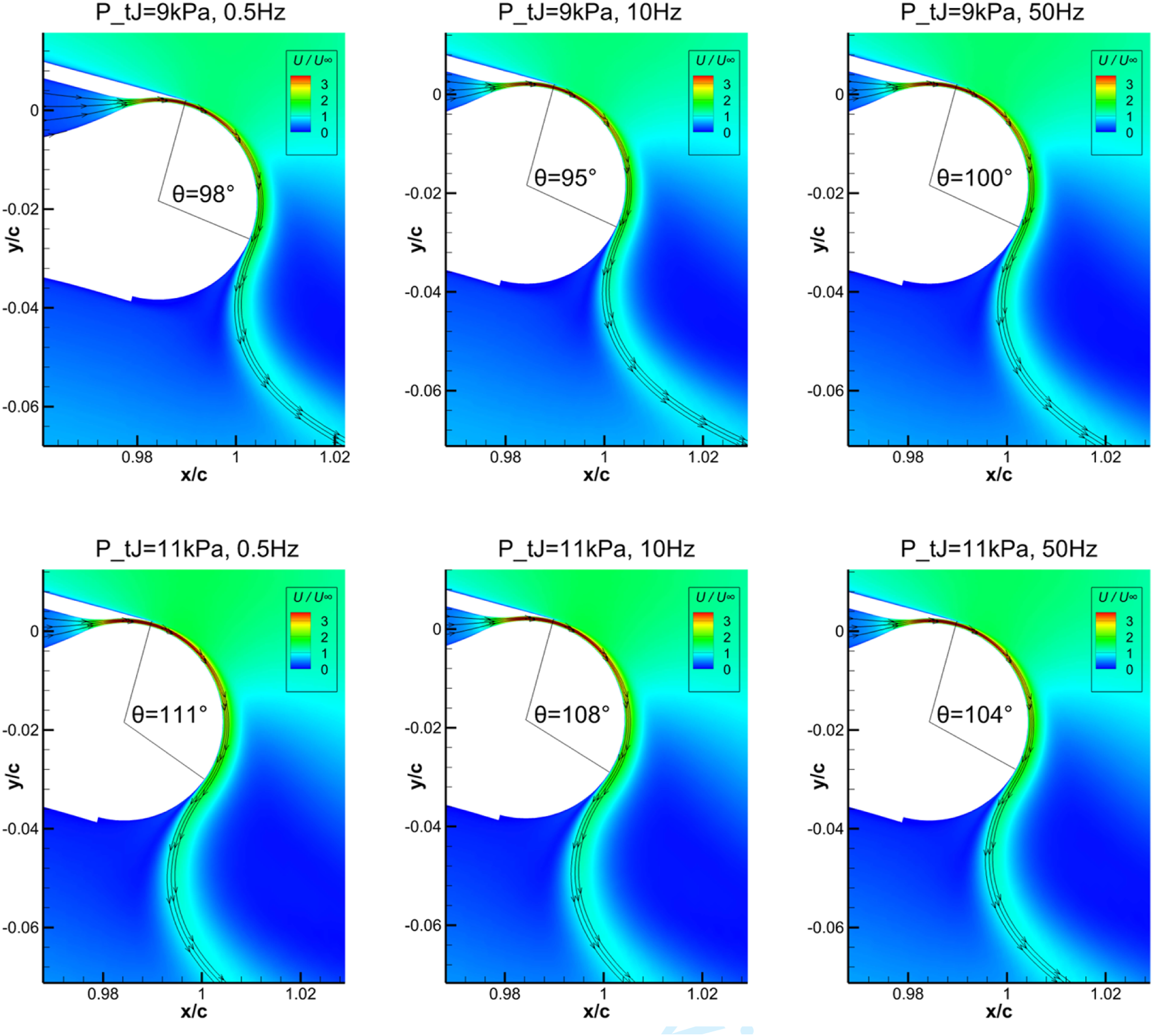

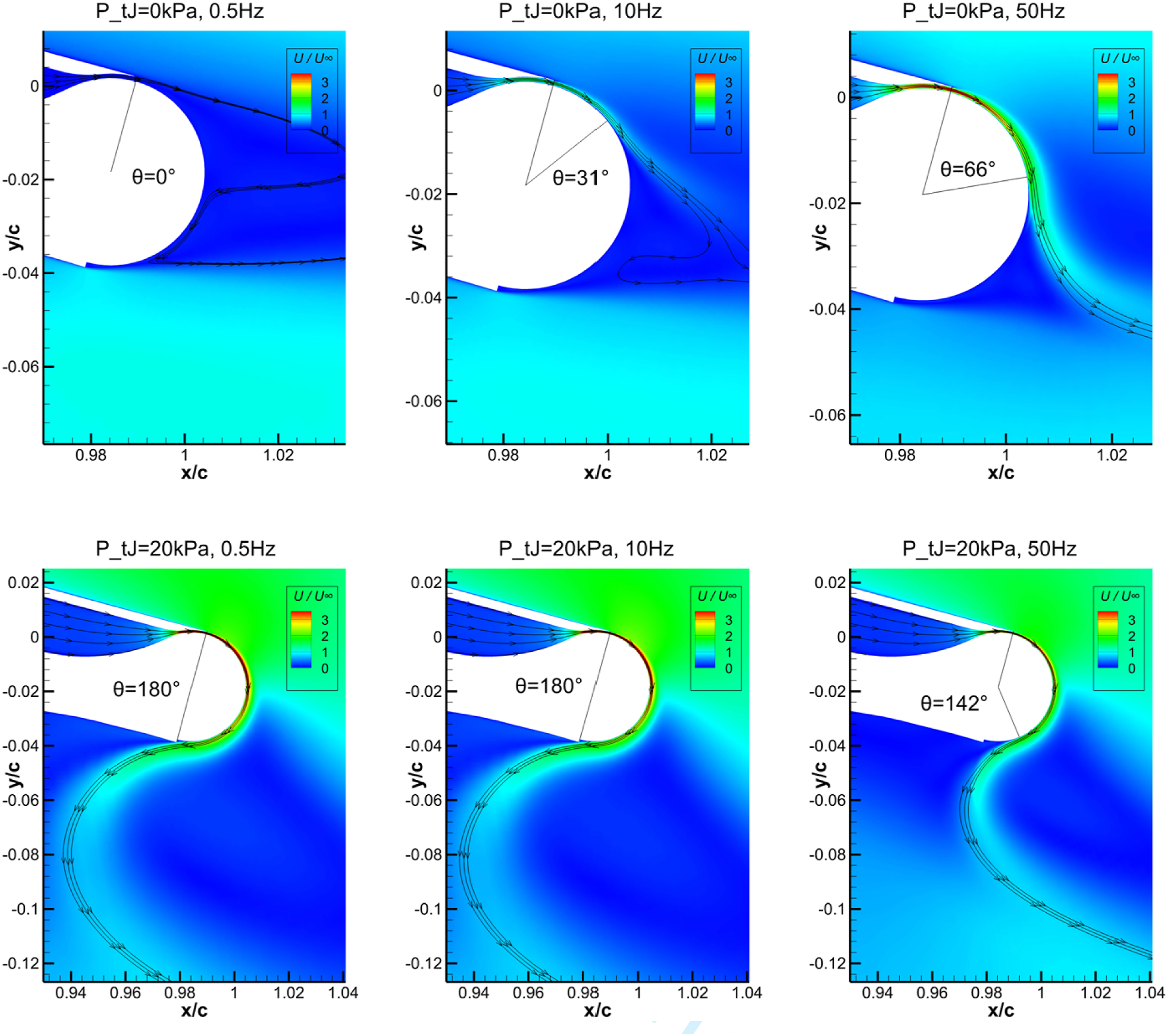
In both Figures 15 and 16, the stagnation point is in unsteady movement within the range between 0 − 180°, there is no significant vortex shedding or unexpected separation. The shape of the jet is predictable and repeatable with various P_tJ inputs between 0.5 Hz and 50 Hz. This system is close to a Linear time-invariant system (LTI system), which means, within the range of the simulated working conditions, the control theory with transfer functions can be used to analyse the system. This will be discussed in the next section.

Circulation control algorithm design & CFD verification

Figure 17 shows the block diagram of the feedback circulation control system. The architecture in Figure 17(a) is used for tuning the controller, where the transfer function of the aerodynamics plant model, G(s), and the wind gust model, G_d(s), are to be identified, $C_{L_{s s}}$ is the reference command, and K(s) is the circulation control algorithm to be designed. Here K(s) can be any control algorithm, including the classical Single-input single-output (SISO) controller in the frequency domain, or Multi-input multi-output (MIMO) controller in the time domain, and the machine-learning based algorithms. The simple PID controller is used to test the closed-loop architecture, future research will also focus on more sophisticated algorithms for K(s). For PID, an initial tunning is necessary to ensure the system is stable. G(s) is only used for PID tuning and it is a low-order transfer function model of the circulation control actuation system in the frequency domain, it has a relatively low accuracy compared to the CFD or wind tunnel tests, and does not represent the nonlinearity flow details. However, transfer function model is much easier to calculate the stablity in various input frequencies. A trial-and-error method is used to identify G(s) to fit the frequency behaviour shown in Figure 12, where the input is P_tJ, the output is C_L within a frequency range between 0.5 Hz to 50 Hz. Different orders of transfer functions have been tried and a best fit function was found. The final K(s) and G(s) will be introduced later in this section.

Figure 17.

The schematic of the system: (a) for controller tuning, (b) for CFD in the loop testing.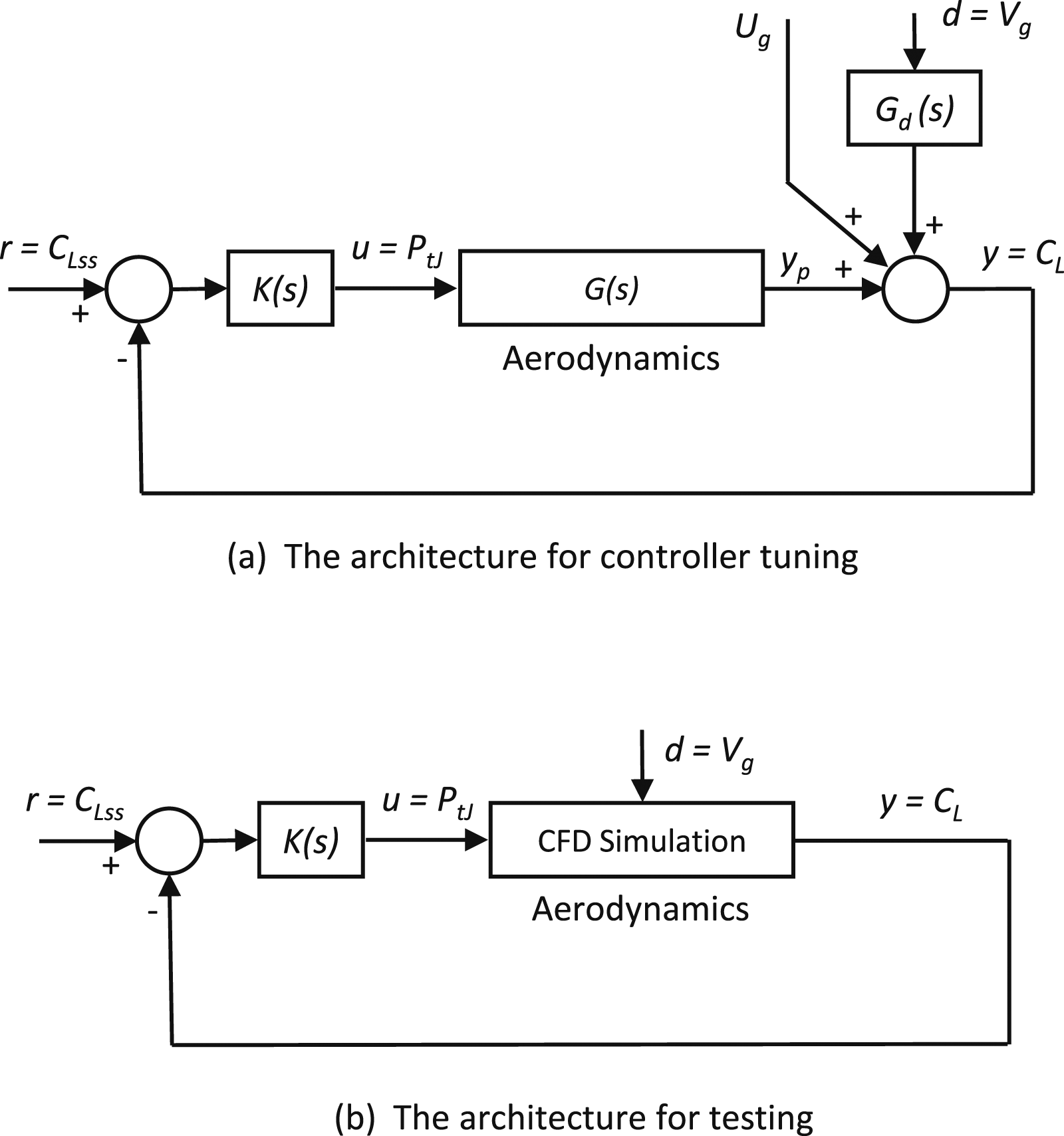

The vertical wind gust has a dominant effect on lift perturbations than the axial wind gust as confirmed in Figure 13. We only consider the vertical wind gust in the control design. The maximum loading due to vertical wind gusts is also one of the primary considerations for wing structure design. Once the controller, K(s), is designed, we verify the controller performance in the CFD simulations. Figure 17(b) shows the CFD solver in the control loop for the verification process, where the gust input, d = V_g, becomes a variable for the far field boundary of the CFD simulations.

The Closed-loop CFD shown in Figure 17(b) works in the following process: Firstly, the control law is programmed in C, and integrated into the UDF (User Defined Function) in Fluent. During the solving process, the program was called at the end of each time step. The controller can obtain the pressure and force information from the API (Application Programming Interface) functions in the solver, which can be treated as virtual ‘sensors’. It reads the instantaneous C_L, duration of the physical time, and the C_L in the previous time step, as input parameters, then calculate the P_tJ with K(s). Finally the new P_tJ is applied to the inlet boundary in the plenum for the next time step. At the same time, the instantaneous gust d = V_g is also calculated in the program, which is a pre-defined function of time.

To design the circulation control algorithm, one of the standard system identification methods uses the frequency responses shown in Figure 12. Consider the case of M = 0.1 and P_tJ = 10 kPa in Figure 12 to design the circulation feedback controller. We use the system identification toolbox in Matlab, where the identification method chooses the best algorithm among several optimization algorithms.⁶⁰ The system identification finds a second-order transfer function as follows:

G_{(s)} = \frac{- 5.174 \times 10^{5} s + 3.907 \times 10^{8}}{s^{2} + 5.26 \times 10^{6} s + 3.947 \times 10^{8}}

(8)

As shown in Figure 18, it fits the frequency response almost perfectly.

Figure 18.

System identification for the lift response at M = 0.1, P_tJ = 10 kPa.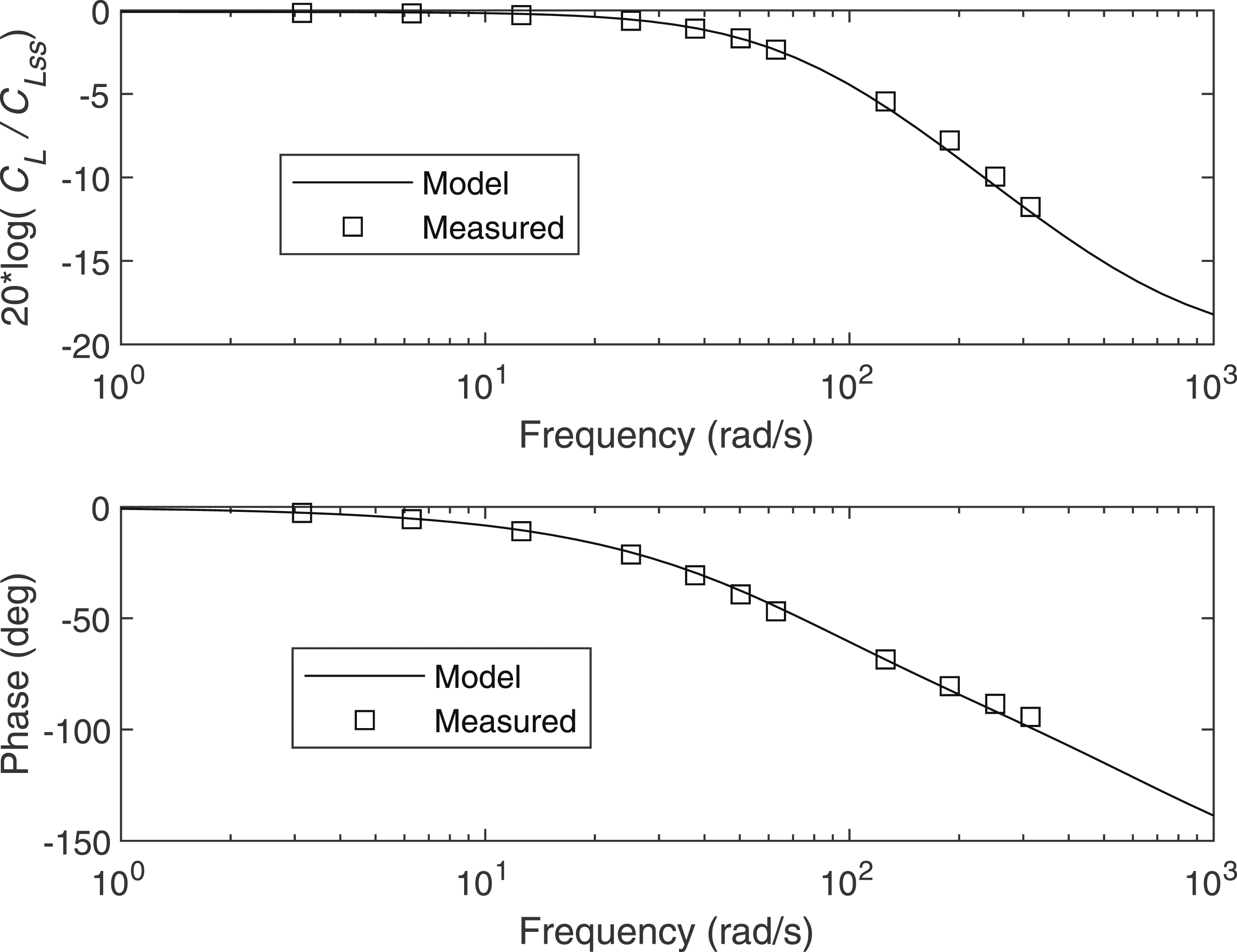

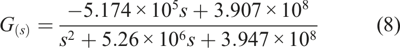
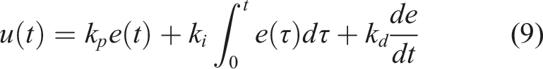
Among many feedback control algorithm, the Proportional-Integral-Derivative (PID) control are the most widely used algorithm proven by its simplicity and effectiveness.⁶¹ Based on the system identified, (8), which is a stable second-order system, the PID is also an appropriate choice. The PID controller structure is given by

u (t) = k_{p} e (t) + k_{i} \int_{0}^{t} e (τ) d τ + k_{d} \frac{d e}{d t}

(9)

where k_p, k_i and k_d are the gains to be determined, and e(t) is the error equal to

r - y = C_{L_{s s}} - C_{L}

. The gains was tuned to achieve a settling time of approximately 0.04 s for a step input of

r = C_{L_{s s}}

, giving k_p = 1.78, k_i = 0.0032, k_d = 0.0061.

To test the gust suppression performance of the PID controller, the same sinusoidal vertical gust profile that has been implemented for Figure 13 is used as the output disturbances. The maximum variation of C_L with and without controller is compared, providing (controlled C_L)/(uncontrolled C_L) in different frequencies. Figure 19 shows that the unsteady lift is dramatically reduced by 81.3% for low frequency gusts at 0.5 Hz. For other frequencies, the controller also effectively suppresses the gusts.

Figure 19.

Gust suppression performance of the tuned PID controller with identified plant model, simulated without CFD.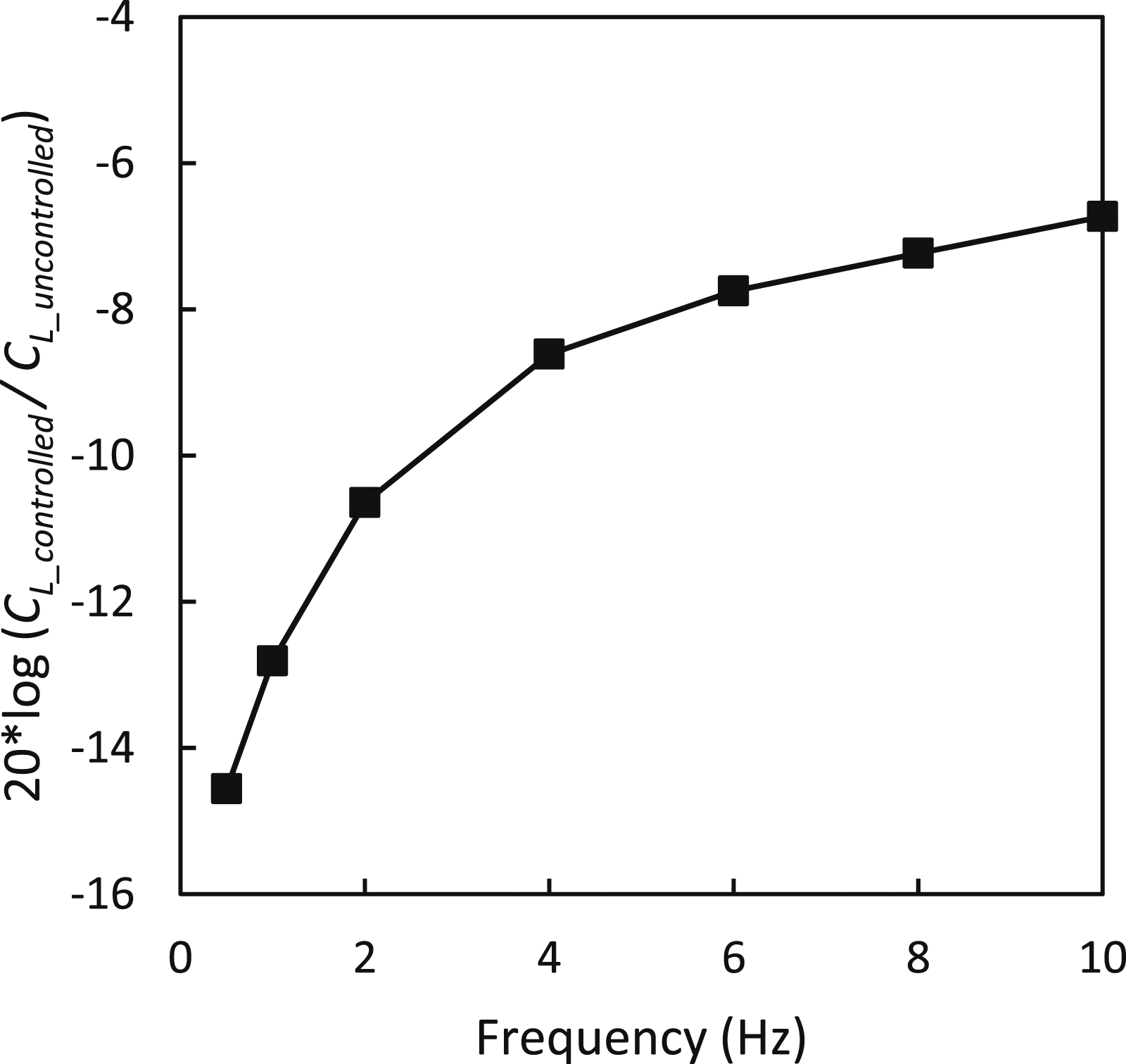

To verify the performance of the PID controller we couple the controller to the Fluent URANS solver. The solver provides real-time gust alleviation control for the GACC aerofoil. We implement the PID controller in the Fluent URANS using the UDF script. The UDF script in the unsteady CFD simulation allows the PID controls the lift by adjusting the nozzle pressure ratio in response to wind gust loadings.

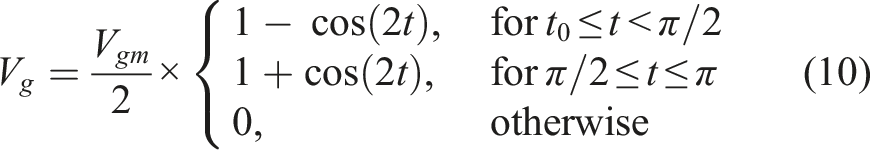
A 1-cosine vertical gust profile used in the CFD simulations is given by⁶²

V_{g} = \frac{V_{g m}}{2} \times {\begin{cases} 1 - \cos (2 t), & for t_{0} \leq t < π / 2 \\ 1 + \cos (2 t), & for π / 2 \leq t \leq π \\ 0, & otherwise \end{cases}

(10)

where the maximum vertical gust velocity, V_gm, is equal to 7% of the freestream velocity, t₀ is the gust initiated time equal to 3s, and t is the time in seconds. The profile is shown in the top figure in Figure 20.

Figure 20.

The time-history variation of the variables under 1-cosine vertical gust at M = 0.1, simulated with CFD.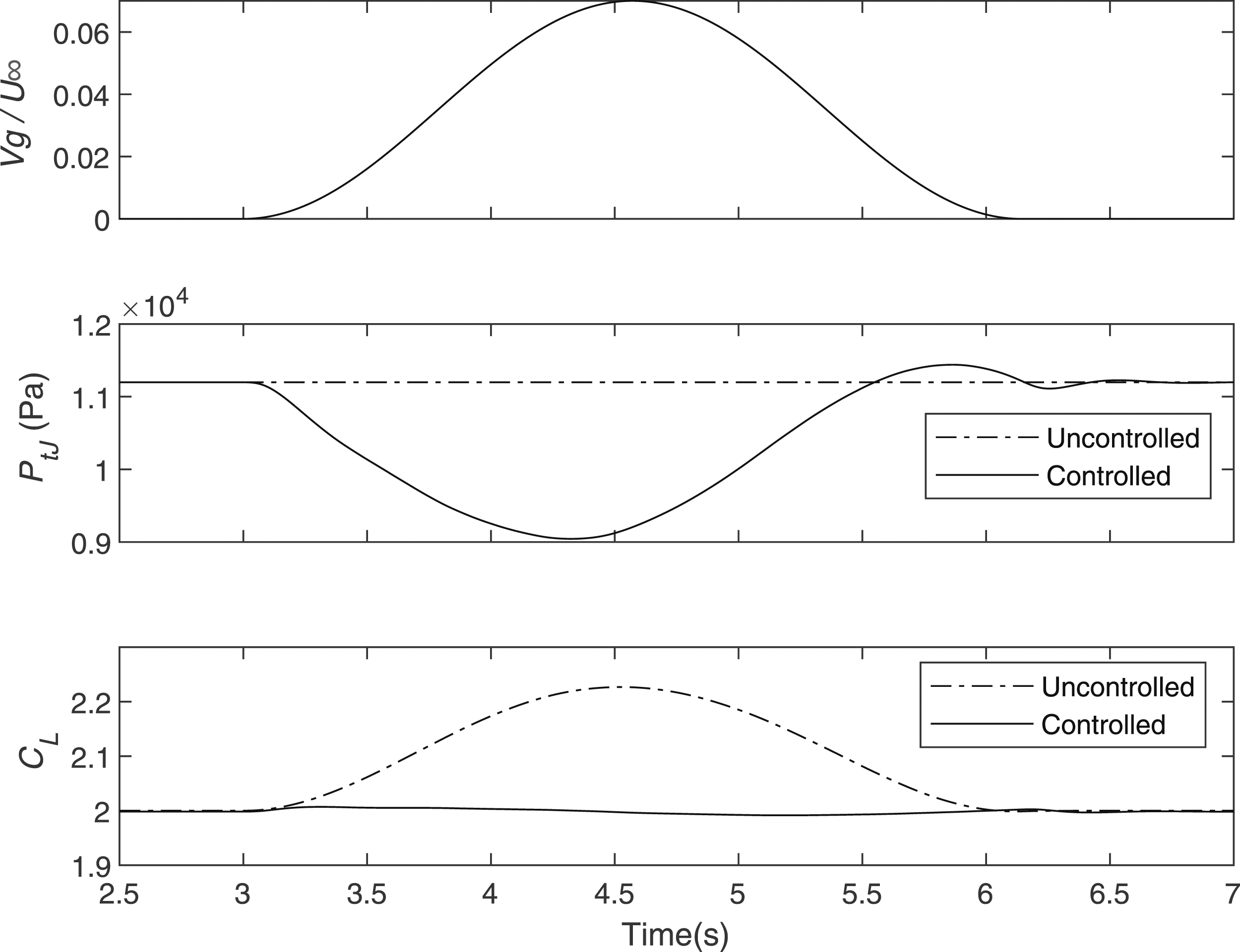

The CFD simulation coupled with the control algorithm is equivalent to a wind tunnel experiment conducted by Kerstens et al.²⁹ We acquire the wind gust measurements from the CFD simulation variables at each time step. The measured values are fed to the PID controller through the UDF, which calculates the nozzle pressure value. The nozzle pressure value controls the circulation in the CFD simulation for the next time step calculations. This framework to evaluate the circulation control performance is cost-effective and flexible compared to a wind tunnel experiment.

Figure 20 shows the CFD simulation results of the circulation control system in the time domain. For the uncontrolled case with a constant plenum chamber pressure equal to 11.1 kPa, the lift increases caused by the vertical gust after t = 3s. On the other hand, when the circulation controller is active, the chamber pressure reacts and successfully maintains a constant lift in response to a gust of wind. The chamber pressure decreases rapidly, and the effective lift coefficient remains the same value as before the wind gust, while the lift for the uncontrolled case increases by 0.2 from the constant value. There is no significant overshoot or oscillation. When the circulation control is used on an aircraft, it would significantly reduce the vertical gust loading applied on the wing.

The CFD simulation coupled with the closed-loop controller has the following advantages,

In each time step, the flow field is fully resolved by RANS equations, the simulated flow is very close to physical experiments, compared to the conventional control design method based on linearised low order empirical models. As the circulation control involves non-linear complex behaviours such as boundary-layer separation, near wall jet flows and entrainment, conventional modelling methods such as transfer functions are not appropriate. They are unable to model the stalling, flow hysteresis, lift fluctuations due to vertex shedding. However, the coupled CFD simulation and control algorithm can simulate these non-linearities within a high-fidelity flow field.

In comparison, Notger and Rudibert presented a similar method in 2010²⁷ to control the flow separation on a mechanical flap in a steady-state flow condition. Their approach used a reduced order mathematical model to represent the flow control device in the system. While in this research the simulation was potentially more accurate and solved the URANS equations for the control loop so that the transient flow field during the disturbance could be obtained. Another similar research conducted by Li et al.,⁴² only considered a stationary aerofoil in a pre-defined gust profile without any feedback controller. At the time of writing, the present research seems to be the first time that a close-loop gust alleviation simulation based on circulation control has been conducted.

There are a few examples where the present ‘closed loop CFD’ is more suitable than the conventional simulation methods for controller design:

Firstly, this method is beneficial for some advanced control algorithms such as the adaptive slope-seeking⁶³ method. The algorithm creates high-frequency waves to the actuator which further augments the lift. The linearised model can not capture such a coupling effect.

For some advanced machine-learning-based algorithms,⁶⁴ they require parameters tunning and testing with massive data sets. The linear model can not be used for training model since it does not have enough accuracy. The wind tunnel experiments and flight tests have limited DoF, or limited flight envelope and not economical when the model needs massive training and tunning process.

The present closed loop CFD method is also ideal for analysing the sharp-edge gust encountering problems. When an aircraft flies into a gust with a sharp edge, the flow direction and velocity change abruptly, this happens in ‘wind shear’ conditions. It results sudden change in the angle of attack, which may lead to a dynamic stall. The transient CFD solver can capture the development of the stalling effect.

Finally, in the stall-recovery or spin-recovery manoeuvre, where different control inputs have dramatically different results. The wing and control surfaces are in off-design condition so there is no empirical model for testing control algorithms. The present method has no restrictions for such simulations.

In summary, Table 1 compared different test methods for a problem that coupled with aerodynamic and control algorithms. The framework provided in this paper filled the gap between linearised model simulation, wind tunnel test and flight test.

Table 1.

Comparison of different test methods.

Test method	Motion	Nonlinear aerodynamic effects	Control algorithm	Cost
Simulation with liner model	6 DoF	Linearised aerodynamic model	Testing and tunning	Low
Closed loop CFD	6 DoF	High order aerodynamic model	Testing and tunning	Low
Wind tunnel	≦ 3 DoF	Realistic flow	Difficult to implement	High
Flight test	6 DoF	Within the flight envelope	Only testing	High

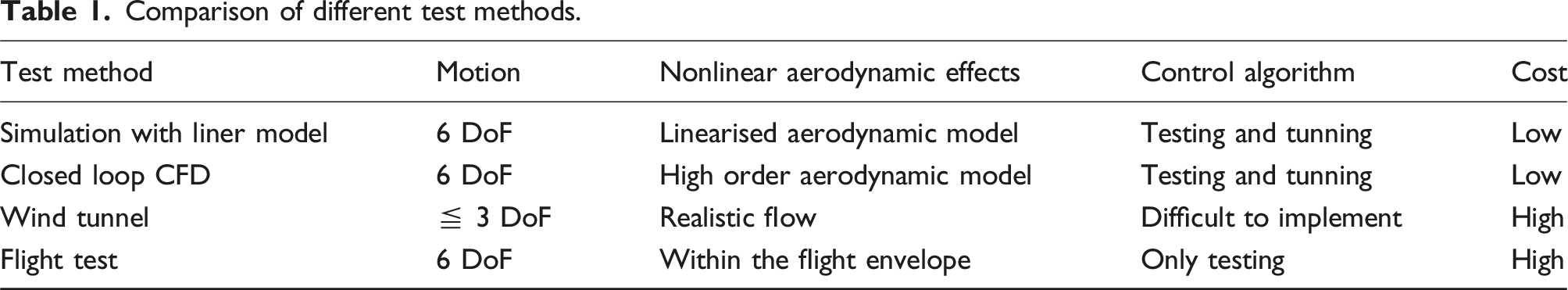
The Motion column indicates the degree of freedom (DoF) that each method can achieve. The simulation methods can achieve 6 DoF that covers all the aircraft motions with velocity or rotational gust disturbance from different axes. Wind tunnel experiments are usually restricted by the test section and therefore have limited DoF. The flight test is realistic but very risky to perform in off-design conditions or outside its flight envelope.

The Nonlinear aerodynamic effects include dynamic stall, hysteresis effect, and flow separation. They are usually associated with off-design conditions and unconventional configurations, such as the circulation control wing, the linearised model is not sufficient to cover such effects. Whereas the flight test method can not capture the flow field around the aircraft, and has restricted working conditions (e.g. small angle of attack).

For the control algorithm research, the present closed loop CFD can tune and test any complex algorithms, which is more flexible compared to other methods. Also has a lower cost compared to wind tunnel and flight test.

Conclusions

We provide a novel simulation framework that combines unsteady CFD simulation and a control algorithm. The control algorithm is integrated in the solver and automatically modifies the boundary condition in each time step, according to the instantaneous results solved in the previous time step. The framework is used to simulate gust alleviation with circulation control.

The dynamic characteristics have been investigated with a sinusoidal plenum chamber pressure using transient CFD simulations. The CFD simulations obtain the lift frequency responses to the chamber pressure and the wind gusts. The system identification algorithm provides the transfer functions, and the PID controller uses the transfer function to tune the control gains. The effectiveness of the PID controller to compensate the vertical wind gusts is validated using the CFD simulation coupled with the controller. The proposed CFD simulation method successfully demonstrates the effectiveness of closed-loop circulation control in unsteady flows. The framework has the potential to be used for various nonlinear control applications involving unsteady fluids, where accurate models are difficult to achieve due to the complex nature of turbulent flows.

Footnotes

Acknowledgments

The authors gratefully acknowledge the funding received towards the first author’s PhD from the China Scholarship Council. This work was undertaken on ARC3, part of the High Performance Computing facilities at the University of Leeds, UK.

Declaration of conflicting interests

The author(s) declared no potential conflicts of interest with respect to the research, authorship, and/or publication of this article.

Funding

The author(s) disclosed receipt of the following financial support for the research, authorship, and/or publication of this article: This work was supported by the China Scholarship Council.

ORCID iD

Shaoze Li

References

Englar

. Development of the a-6/circulation control wing flight demonstrator configuration. Technical report. DTIC Document, 1979.

Englar

Hemmerly

Moore

, et al. Design of the circulation control wing stol demonstrator aircraft. J Aircraft 1981; 18(1): 51–58. DOI: 10.2514/3.57463.

Englar

Jones

Allan

, et al. 2-d circulation control airfoil benchmark experiments intended for cfd code validation. In 47th AIAA Aerospace sciences meeting including the new horizons forum and aerospace exposition, p. 902. 5-8 January 2009. Orlando, Florida. DOI: 10.2514/6.2009-902.

Kind

. A calculation method for circulation control by tangential blowing around a bluff trailing edge. Aeronaut Q 1968; 19(3): 205–223. DOI: 10.1017/S0001925900004613.

Wood

Nielsen

. Circulation control airfoils-past, present, future. In 23rd Aerospace Sciences Meeting, p. 204. 14-17 January 1985. Reno, NV, U.S.A. DOI: 10.2514/6.1985-204.

Novak

Cornelius

Roads

. Experimental investigations of the circular wall jet on a circulation control airfoil. In 25th AIAA Aerospace Sciences Meeting, p. 155. 24-26 March 1987. Reno, NV, U.S.A. DOI: 10.2514/6.1987-155.

Ghee

Leishman

. Unsteady circulation control aerodynamics of a circular cylinder with periodic jet blowing. AIAA J 1992; 30(2): 289–299. DOI: 10.2514/3.10916.

Cutbill

. A study of the turbulent flow of a high speed Coanda jet. PhD Thesis. Durham University, 1998.

Paterson

Baker

Kunz

, et al. Rans and detached-eddy simulation of the nccr airfoil. In 2004 Users Group Conference (DOD_UGC’04)2004. IEEE, pp. 112–122. 07-11 June 2004. Williamsburg, VA, USA. DOI: 10.1109/DOD_UGC.2004.38.

10.

Jones

Joslin

. Proceedings of the 2004 nasa/onr circulation control workshop. Technical report 2005.

11.

Buonanno

Cook

. Flight dynamic simulation of a flapless flight control uav. In 25th International Congress of the Aeronautical Sciences. 3-8 September 2006, Hamburg, Germany.

12.

Gross

Fasel

. Cfd for investigating active flow control. In 4th Flow Control Conference, p. 4310. 23-26 June 2008, Seattle, Washington. DOI: 10.2514/6.2008-4310.

13.

Nishino

Hahn

Shariff

. Large-eddy simulations of a turbulent Coanda jet on a circulation control airfoil. Physics of fluids 2010; 22(12): 125105. DOI: 10.1063/1.3526757.

14.

Nishino

Shariff

. Numerical study of wind-tunnel sidewall effects on circulation control airfoil flows. AIAA J 2010; 48(9): 2123–2132. DOI: 10.2514/1.J050328.

15.

Rumsey

Nishino

. Numerical study comparing rans and les approaches on a circulation control airfoil. Int J Heat Fluid Flow 2011; 32(5): 847–864. DOI: 10.1016/j.ijheatfluidflow.2011.06.011.

16.

Rosen

Kanistras

Saka

, et al. Design and development of a control scheme for the uc2av: Unmanned circulation control aerial vehicle. In 55th AIAA Aerospace Sciences Meeting, p. 1528. 9-13 January 2017 Grapevine, Texas. DOI: 10.2514/6.2017-1528.

17.

McGowan

Gopalarathnam

Jones

. Analytical and computational study of adaptive circulation control airfoils. In 22nd Applied Aerodynamics Conference and Exhibit, p. 4721. 16-19 August 2004. Providence, Rhode, Island. DOI: 10.2514/6.2004-4721.

18.

Buonanno

. Aerodynamic circulation control for flapless flight control of an unmanned air vehicle, 2009.

19.

Savvaris

Buonanno

Jamil

, et al. Design and development of the demon uav fluidic flight control system. In AIAA Infotech@ Aerospace (I@ A) Conference, p. 4820. 19-22 August, 2013. Boston, MA. DOI: 10.2514/6.2013-4820.

20.

Cagle

A wind tunnel model to explore unsteady circulation control for general aviation applications. In 22nd AIAA Aerodynamic Measurement Technology and Ground Testing Conference, p. 3240. 24-26 June 2002, St. Louis, Missouri. DOI: 10.2514/6.2002-3240.

21.

Swanson

Rumsey

Anders

. Progress towards computational method for circulation control airfoils. In 43rd AIAA Aerospace Sciences Meeting and Exhibit, p. 89. 10-13 January 2005. Reno, NV. DOI: 10.2514/6.2005-89.

22.

Rogers

Donnelly

. Characteristics of a dual-slotted circulation control wing of low aspect ratio intended for naval hydrodynamic applications. In 42nd AIAA Aerospace Sciences Meeting and Exhibit, p. 1244. 5-8 January 2004. Reno

Nevada.

DOI: 10.2514/6.2004-1244.

23.

Paschal

Neuhart

Beeler

, et al. Circulation control model experimental database for cfd validation. In 50th AIAA Aerospace Sciences Meeting including the New Horizons Forum and Aerospace Exposition, p. 705. 9-12 January 2012. Nashville, Tennessee. DOI: 10.2514/6.2012-705.

24.

Golden

Marshall

. Design and performance of circulation control flap systems. In 48th AIAA Aerospace Sciences Meeting Including the New Horizons Forum and Aerospace Exposition, p. 1053. 4-7 January 2010. Orlando, Florida. DOI: 10.2514/6.2010-1053.

25.

Taha

Rezaei

. On the dynamics of unsteady lift and circulation and the circulatory-non-circulatory classification. In AIAA Scitech 2019 Forum, p. 1853. 7-11 January 2019. San Diego, California. DOI: 10.2514/6.2019-1853.

26.

Hahn

König

. Advanced technologies testing aircraft system flight test and simulation results of the advanced gust management system lars. In Guidance, Navigation and Control Conference, p. 4343. 10-12 August 1992. Hilton Head Island, SC, U.S.A. DOI: 10.2514/6.1992-4343.

27.

Heinz

King

Höll

, et al. Numerical investigation of robust closed-loop flow control of a high-lift configuration. In 5th Flow Control Conference, p. 4967. 28 June 2010 - 01 July 2010, Chicago, Illinois. DOI: 10.2514/6.2010-4967.

28.

Xiaoping

Zhou

, et al. Application of active flow control technique for gust load alleviation. Chin J Aeronaut 2011; 24(4): 410–416. DOI: 10.1016/S1000-9361(11)60048-4.

29.

Kerstens

Pfeiffer

Williams

, et al. Closed-loop control of lift for longitudinal gust suppression at low Reynolds numbers. AIAA J 2011; 49(8): 1721–1728. DOI: 10.2514/1.J050954.

30.

Nelson

. Flight stability and automatic control. New York: WCB/McGraw Hill, 1998, vol 2.

31.

Jones

Lin

Allan

, et al. Overview of cfd validation experiments for circulation control applications at nasa. In 2008 International powered lift Conference, 22-24 Jul 2008, London, United Kingdom.

32.

Küssner

. Zusammenfassender bericht über den instationären auftrieb von flügeln. Luftfahrtforschung 1936; 13(12): 410–424.

33.

Jones

. The unsteady lift of a wing of finite aspect ratio. Technical report, 1940.

34.

Stalnov

. Closed-loop active flow control for uavs. Advanced UAV Aerodynamics, Flight Stability and Control: Novel Concepts, Theory and Applications 2017: 447–464. DOI: 10.1002/9781118928691.ch13.

35.

Michailidis

Agha

Kanistras

, et al. A controller design framework for a nextgen circulation control based uav. In 2017 IEEE Conference on Control Technology and Applications (CCTA). IEEE, pp. 1542–1549. 27-30 August 2017. Maui, HI USA. DOI: 10.1109/CCTA.2017.8062676.

36.

Allan

Juang

Raney

, et al. Closed-loop separation control using oscillatory flow excitation. Technical report; 2000.

37.

Glauser

Higuchi

Ausseur

, et al. Feedback control of separated flows. In 2nd AIAA Flow Control Conference, p. 2521. 28 June 2004 - 01 July 2004. Portland, Oregon. DOI: 10.2514/6.2004-2521.

38.

King

Becker

Garwon

, et al. Robust and adaptive closed-loop control of separated shear flows. In 2nd AIAA Flow Control Conference, p. 2519. 28 June 2004 - 01 July 2004. Portland, Oregon. DOI: 10.2514/6.2004-2519.

39.

Becker

Garwon

Gutknecht

, et al. Robust control of separated shear flows in simulation and experiment. J Process Control 2005; 15(6): 691–700. DOI: 10.1016/j.jprocont.2004.12.001.

40.

Petz

Nitsche

Becker

, et al. Lift, drag and moment control on a high-lift configuration by means of active flow control. In CEAS/KATnet Conference on Key Aerodynamic Technologies. 20 - 22 June 2005, Deutsche Gesellschaft fr Luft-und. Raumfahrt, European Union Bremen, Germany.

41.

Barzgaran

Quenzer

Zongolowicz

, et al. Low-cost wind tunnel studies of gust alleviation control techniques. International Forum on Aeroelasticity and Structural Dynamics.

42.

Qin

. Airfoil gust load alleviation by circulation control. Aero Sci Technol 2020; 98: 105622. DOI: 10.1016/j.ast.2019.105622.

43.

Keller

Rudnik

. Numerical investigation of engine effects on a transport aircraft with circulation control. J Aircraft 2015; 52(2): 421–438. DOI: 10.2514/1.C032724.

44.

Jones

Viken

Washburn

, et al. An active flow circulation controlled flap concept for general aviation aircraft applications. AIAA paper 2002; 3157(1): 43. DOI: 10.2514/6.2002-3157.

45.

Spalart

Allmaras

. A one-equation turbulence model for aerodynamic flows. In 30th aerospace sciences meeting and exhibit, p. 439. 6-9 January 1992. Reno, NV, U.S.A. DOI: 10.2514/6.1992-439.

46.

Raveh

. Cfd-based models of aerodynamic gust response. J Aircraft 2007; 44(3): 888–897. DOI: 10.2514/1.25498.

47.

Medina

Mancini

, et al. Revisiting conventional flaps at high deflection rate. AIAA J 2017; 55(8): 2676–2685. DOI: 10.2514/1.J055754.

48.

Zaide

Raveh

. Numerical simulation and reduced-order modeling of airfoil gust response. AIAA J 2006; 44(8): 1826–1834. DOI: 10.2514/1.16995.

49.

Karakaş

. Gust alleviation techniques and design methods of active aeroelastic wing. PhD Thesis. Istanbul Technical University, 2020.

50.

Leishman

. Unsteady lift of a flapped airfoil by indicial concepts. J Aircraft 1994; 31(2): 288–297. DOI: 10.2514/3.46486.

51.

Wright

Cooper

. Introduction to aircraft aeroelasticity and loads. John Wiley & Sons, 2008, vol 20. DOI: 10.2514/4.479359.

52.

von Karman

Sears

. Airfoil theory for non-uniform motion. J Aeronaut Sci 1938; 5(10): 379–390. DOI: 10.2514/8.674.

53.

William R Sears . On the reaction of an elastic wing to vertical gusts. J Aeronaut Sci 1941; 8(2): 64–67.

54.

Ghoreyshi

Greisz

Jirasek

, et al. Simulation and modeling of rigid aircraft aerodynamic responses to arbitrary gust distributions. Aerospace 2018; 5(2): 43. DOI: 10.3390/aerospace5020043.

55.

Shires

. Dynamic response of circulation control for step and sinusoidal inputs. J Aircraft 2023; 60(6): 1761–1772. DOI: 10.2514/1.C037042.

56.

Förster

Breitsamter

. Aeroelastic prediction of discrete gust loads using nonlinear and time-linearized cfd-methods. Journal of Aeroelasticity and Structural Dynamics 2015; 3(3): 17.

57.

Bartels

. Development, verification and Use of gust modeling in the NASA computational fluid dynamics code FUN3D. In: National Aeronautics and Space Administration. Langley Research Center, 2012.

58.

Phillips

Wygnanski

. Use of sweeping jets during transient deployment of a control surface. AIAA J 2013; 51(4): 819–828. DOI: 10.2514/1.J051683.

59.

SMC . SX10 high-speed 2 Port valve. SMC Pneumatics LTD, 2014.

60.

Ljung

. System identification toolbox. The Matlab user’s guide, 2022.

61.

Åström

Hägglund

. The future of pid control. Control Eng Pract 2001; 9(11): 1163–1175. DOI: 10.1016/S0967-0661(01)00062-4.

62.

Cook

. Flight dynamics principles: a linear systems approach to aircraft stability and control. Butterworth-Heinemann, 2012, pp. 462–463.

63.

Henning

Becker

Feuerbach

, et al. Extensions of adaptive slope-seeking for active flow control. Proc IME J Syst Control Eng 2008; 222(5): 309–322. DOI: 10.1243/09596518JSCE490.

64.

Rabault

Kuchta

Jensen

, et al. Artificial neural networks trained through deep reinforcement learning discover control strategies for active flow control. J Fluid Mech 2019; 865: 281–302. DOI: 10.1017/jfm.2019.62.

Closed-loop computational fluid dynamics simulations with time-varying boundary conditions for circulation control

Abstract

Keywords

Introduction

Circulation control system & CFD validation

The simulation model

Steady validation

Unsteady validation

Frequency response of circulation control system

Circulation control algorithm design & CFD verification

Conclusions

Footnotes

Acknowledgments

Declaration of conflicting interests

Funding

ORCID iD

References