
Abstract
Unsteady, viscous compressible flow is numerically simulated within first two stages of a low pressure turbine of a gas turbine engine under different clocking of its stator blades rows. Zonal DES turbulence modeling has been used for flow simulations. Time-dependent wake flow trajectory is modeled and visualized within the blades passages. All characteristics of the passage wake flow, including its V-shape motion, re-orientation, elongation, expansion, and stretching, are properly simulated. Unsteady flow field results together with those of general aerodynamic performance of the optimum and worst clocking cases are presented and compared with each other. Analyses of the flow simulation results showed that the optimum clocking of the blades rows occurs while the upstream wake flow impinges on the downstream stator blade leading edge region. Final results demonstrated that under the optimum clocking of the second stator, the inlet total pressure of the second rotor blades row and its output power increase by 0.1% and 0.336%, respectively. Consequently, efficiency of the second stage increases by 0.35%. In addition, total output power of the whole two stages increases by 0.237%.
Introduction
Wake flow originated from upstream blade rows in a compressible flow multistage turbomachine and their interaction with probable existing shock waves can enforce more complexity to the flow structure.
1
Figure 1 schematically illustrates such a complicated flow. As mentioned by Meneveau and Katz
2
and Rhie et al.,
3
local unsteady internal fluid stresses resulting from movement of the wakes can be typically similar to turbulent stresses and even of higher magnitudes. General view of flow structure within a compressible flow turbomachine stage.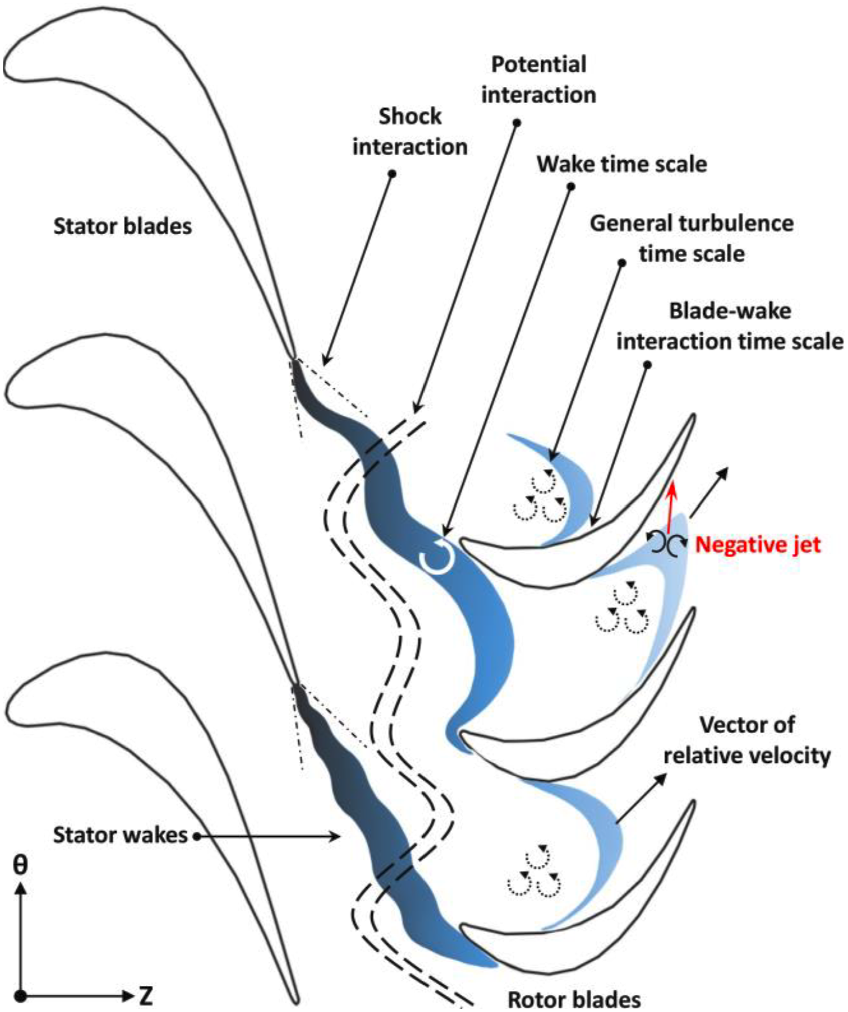
Clocking of blades rows can influence performance of any multistage axial turbomachine, significantly. Optimum circumferential alignment of blades rows (i.e., stator-stator and rotor-rotor) can be useful in increasing whole turbomachine efficiency by controlling upstream stator-rotor wake flow interactions with adjacent downstream stator blades. Precise and detail results can be obtained through proper unsteady numerical simulation; even though, this process is complex and time consuming.
Advent of clocking concept may be referred to experimental investigations of Ladwig. 4 He concluded that the turbine efficiency can be optimized by controlling the upstream wake flow trajectory, especially its impact point on the subsequent blades surfaces. Through experimental studies and unsteady 3-D numerical simulations for clocking analysis of a 2-stage axial turbine, Sharma et al. concluded that aerodynamic performance of a turbine can be improved by adjusting relative position of the fixed blades row. 5
Quasi 3-D unsteady analyses of a 1.5 stage compressor, executed by Dorney et al., have shown that stator clocking can result in efficiency gain of 0.6–0.7%. 6 They concluded that this advantage is mainly due to the modification of the wake flow trajectory through the optimum clocking, which result in reduction in the existing losses. Cizmas and Dorney through their investigations on a 3-stage axial turbine concluded that clocking of the second stage blades is more efficient than that of the third stage. 7
Results of experimental analyses on a 2-stage axial turbine, carried out by Huber et al., have shown 0.8% increase in its total efficiency under the optimum clocking of the first stator blades row. 8 Griffin et al. have performed 2-D viscous unsteady numerical simulations to study stator clocking effects on the aerodynamic performance of the turbine which was tested by Huber at mid-span. 9 Their numerical analysis correctly predicted the optimum clocking positions corresponded to the maximum efficiency. But the magnitude of the predicted efficiency was less than that experimentally observed, due to 2-D nature of the analysis.
Arnone et al. have performed full and quasi 3-D numerical simulations to investigate clocking effects in a 3-stage low pressure turbine (LPT) by solving the unsteady Navier–Stokes equations. 10 They showed that rotational speed of shaft, during take-off and cruise conditions, has no effect on the optimum clocking position.
3-D unsteady viscous flow computations have been performed by Reinmöller et al. for clocking studies of a 1.5-stage axial turbine. 11 Total pressure loss of the second stator, considered as a criterion for the performance studies, was chosen to find the optimum clocking position of the second stator blades. In addition, they have presented clocking results on the potential field of the second stator in terms of the turbulence intensity and absolute velocity behind the second stator. Through 3-D unsteady flow simulations of a 1.5-stage axial turbine, Arnone et al. concluded that the efficiency would be the maximum when the wake flow impinges on the second stator leading edge region. 12 On the other hand, the minimum efficiency obtains while the wake flow enters the middle space of the blades passage.
Frozen rotor technique for steady and sliding mesh approach for unsteady simulations have been performed by Bohn et al. to study stator clocking effects in a 2-stage axial turbine over six circumferential positions of the blades, using
Bohn et al. numerically showed that through optimum clocking, the efficiency of a 2-stage turbine can be increased by 0.52%. 15 Behr et al. experimentally studied stator clocking effects on the unsteady interaction of stator and upstream secondary flows in a 1.5-stage HPT. 16 They found that stator clocking can be non-uniformly effective in controlling spanwise distribution of pressure loss within the second stator due to highly complex flow structures.
Through researches on rotor-stator blades rows interactions in a twin-shaft turbine, Gaetani concluded that the maximum efficiency can be achieved when the upstream wake impinges on the next stator blade leading edge. 17 He also concluded that at low Reynolds numbers, upstream wakes causes transition to occur while they interact with the blade suction side boundary layer. Although, this transitional flow causes the losses to increase, it makes the boundary layer to encounter with streamwise adverse pressure gradient, and as a result, prompts the flow separation point to move downstream.
An in-house 3-D URANS flow solver for multistage turbomachines has been implemented by Zhu et al. for clocking studies on a 1.5-stage axial turbine.
18
They concluded that minimum outlet total pressure at mid-span of the second stator blades occurs when the upstream wake passes through the middle space of the second stator blades passage. The same experimental result had been concluded by König et al. in a 1.5-stage LPT.
19
Ghenaiet and Touil have investigated clocking in a 2-stage axial turbine using CFX software and
Using potential flow formulation, Swirydczuk concluded that under an optimum clocking position, a special form of upstream wake vortices is shed within the blades passage which increases dynamic pressure and consequently outlet total pressure at blade throat. 22 Other wake tracking analyses can be referred to some researchers like Hodson, 23 Jouini et al., 24 Gombert et al., 25 and Arndt. 26 These researchers reported that the blade-wake interactions can be controlled by clocking mechanism to influence the aerodynamic performance of axial turbines, including turbine efficiency, profile loss, boundary layer transition, and development of the secondary flows.
Additionally, clocking mechanism can be accounted effective in controlling acoustic and heat transfer problems in the axial turbines. All these advantages are the motivations for researchers to study “clocking” effect on other facets. Ghoreyshi and Schobeiri numerically investigated effect of various clocking positions of fuel injectors relative to each other and nozzle guide vanes on the vanes cooling effectiveness. 27 Their results showed that in an optimum clocking position, vanes surface temperature is reduced while the maximum output power is preserved.
In the present research work, flow field within the first two stages of a 4-stage axial turbine of a gas turbine engine is numerically simulated under different clocking of the stator blades. Unsteady, viscous, and compressible flow is solved and results of the optimum clocking position are compared with the worst case. Time-averaged results of aerodynamic performance and instantaneous flow filed due to interaction of the upstream wake with the subsequent blades rows are presented and discussed, qualitatively and quantitatively. There is lack of comprehensive phenomenology of the wake flow structure under various clocking positions in the literature. This shortage serves as a motivation for the present research work to distinguish kinematic of the wake flow along with its transient effects on the fixed and rotating blades loadings. In addition, the method of computation is based on utilizing the Zonal DES, since it produces more uniform and reliable results in comparison to the conventional URANS specially while dealing with separated regions. 28
Model and computational domain
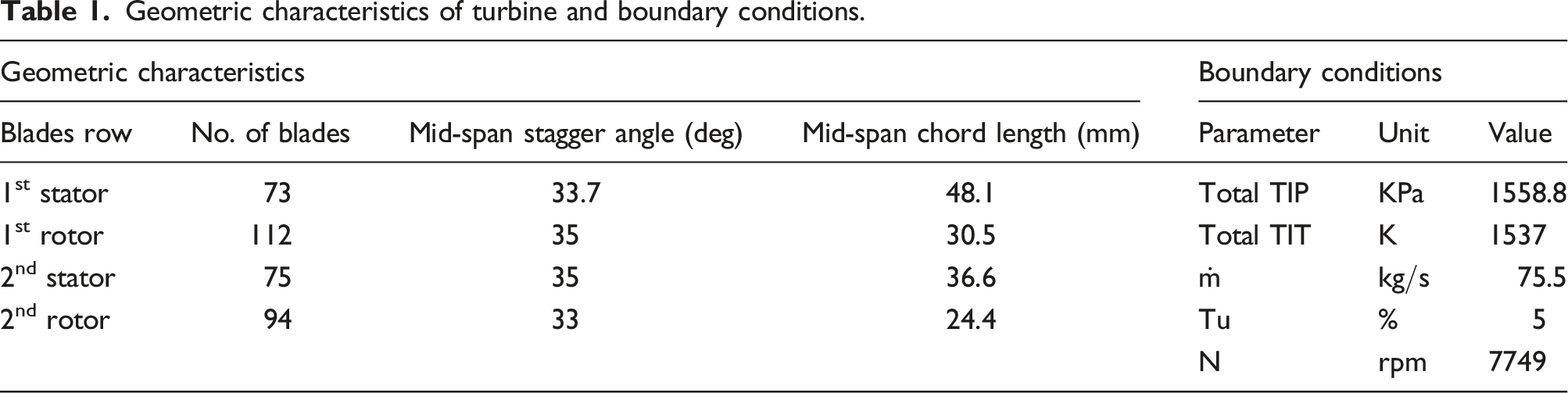
Figure 2 shows 3-D geometry of the model of investigation and blades profiles at mid-span. The model consists of first two stages of a 4-stage LPT of a gas turbine engine. Table 1 summarizes geometric specifications of the blades rows at their mid-spans. Boundary conditions are also introduced in this table. Geometry of first two stages of a low pressure axial turbine. Geometric characteristics of turbine and boundary conditions.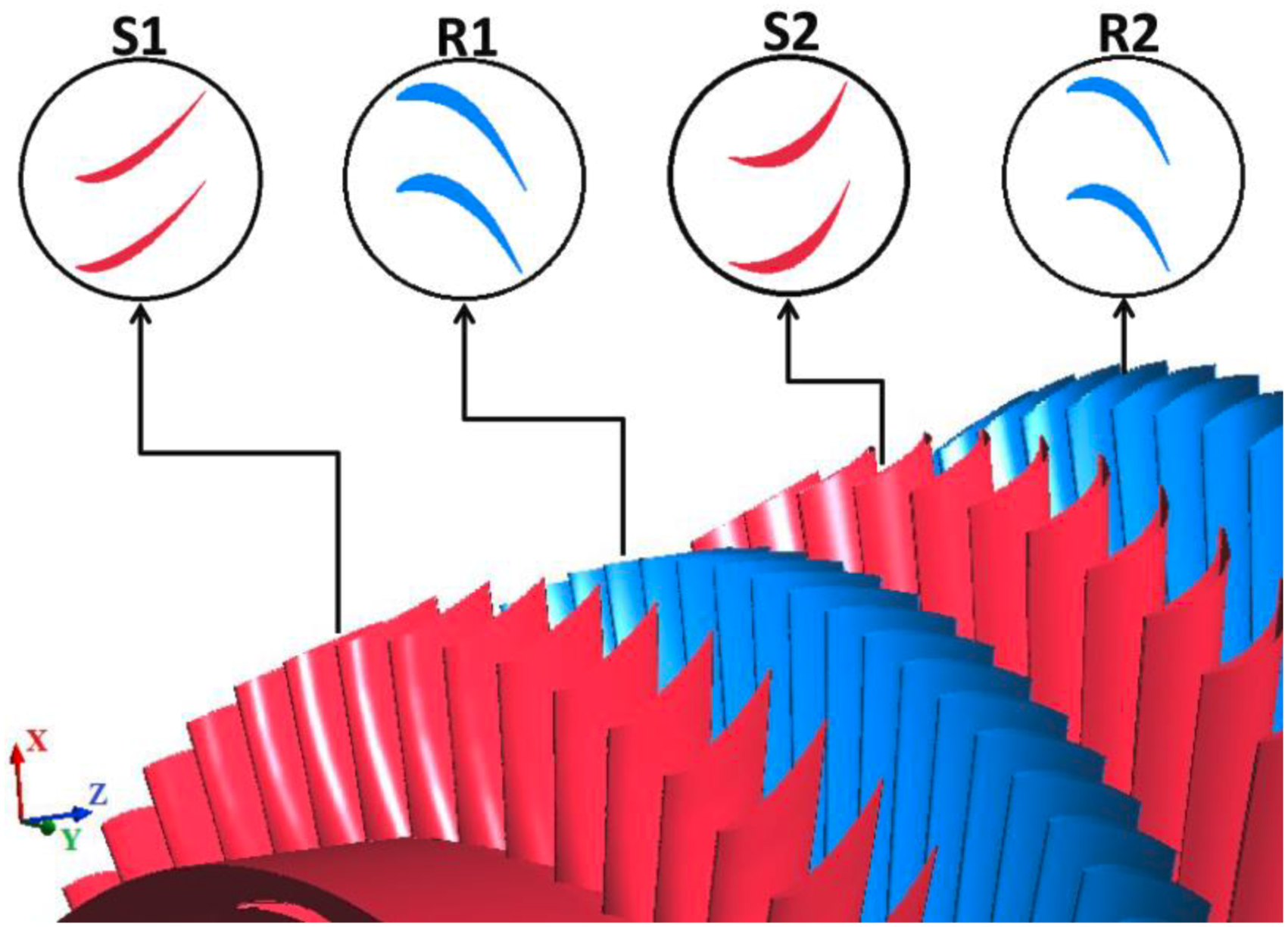
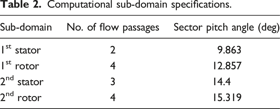
Computational domain is shown in Figure 3. The total pressure and mass flow rate are imposed on the inlet and outlet boundaries, respectively. Solid walls are considered as adiabatic and periodicity condition is used for the circumferential boundaries. Table 2 presents sector information for each region of the computational domain. Computational domain. Computational sub-domain specifications.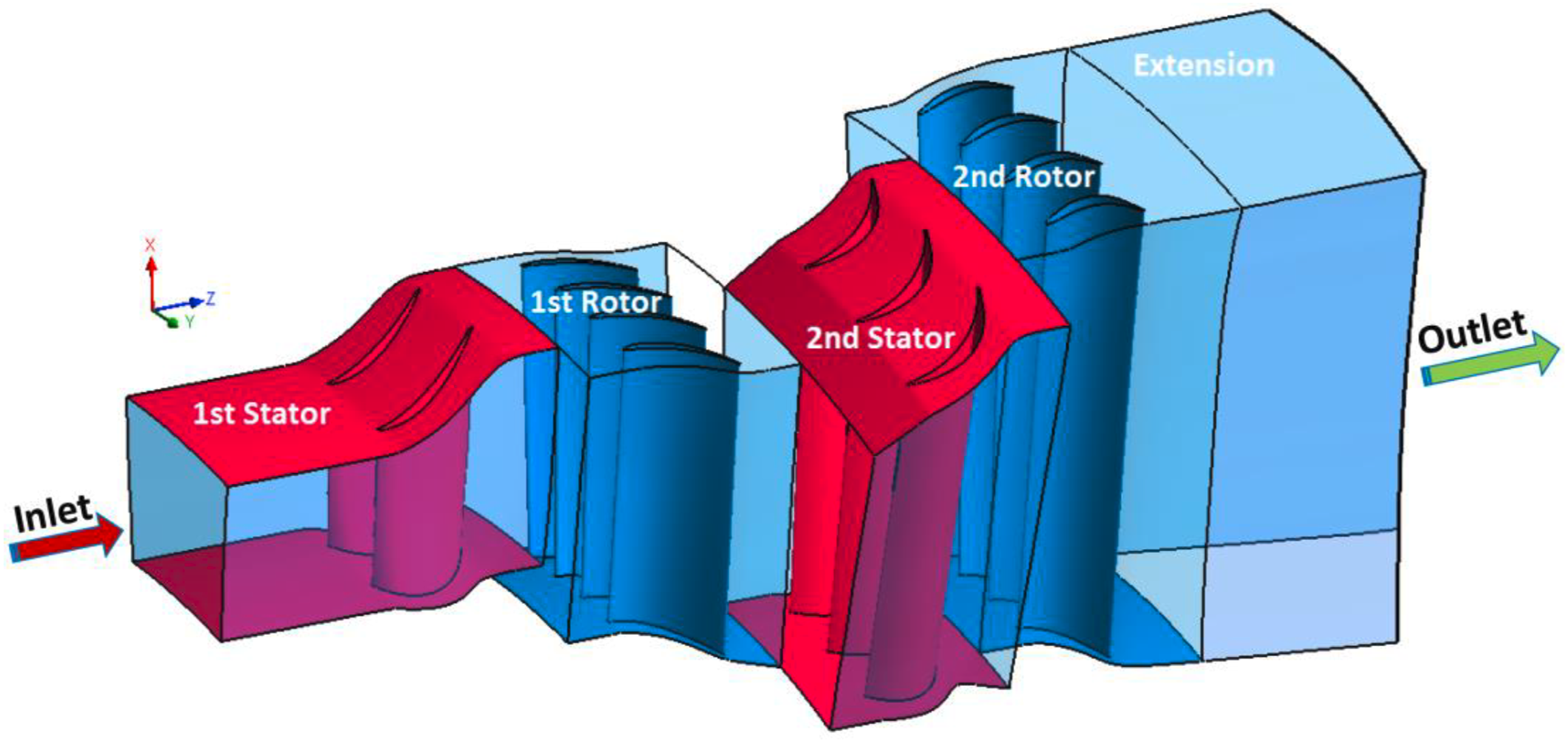
As shown in Figure 4, five clocking positions are applied on the second stator blades row with 0.98° intervals along the circumference. These positions are designated by CLP1 to CLP5. The initial case is also shown by CLP0. Second stator clocking configuration.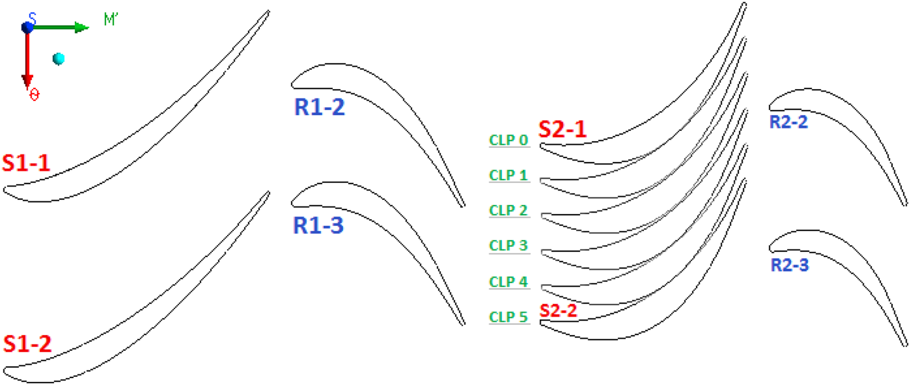
Numerical simulation procedure
Structured mesh system has been applied for the computational domain using the well-known TurboGrid software. Initially, steady simulations based on
Interface between moving and fixed surfaces
While dealing with unsteady simulations, using transient rotor-stator interface technique would be proper for transferring data between different computational domains. In this strategy, while advancing to the next time step, the cell and wall zones will be automatically moved according to the specified translational or rotational velocities. So the new interface-zone intersection will be recalculated and updated. This leads to modeling transitional relative motion between moving and fixed components on each side of the interface with the highest accuracy. Although the results obtained from this technique are very close to the reality, its requirement to large storage spaces and strong hardware usually confines its application.
Governing basic equations
The governing main equations are introduced as follows: - Continuity equation - Momentum equations
Momentum equations for rotating sub-domains of the main solution field are the Navier–Stokes equations in the rotating frame. Since fully coupled solution procedure of velocity and pressure fields is applied through the calculations, these equations are used in the rotating frame based on the absolute velocity. The vector form of the momentum equation is presented by equation (2).
In the above equation, the second and third terms on the right hand side represents centrifugal and Coriolis forces, respectively. The above equation can be re-written in terms of the relative velocities as equation (3). - Energy equation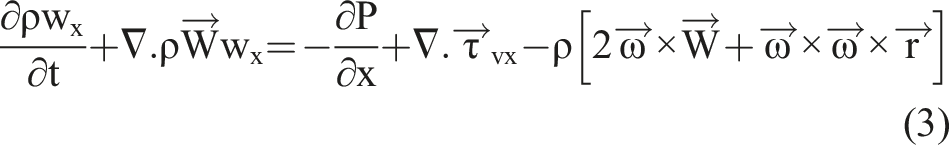
The energy conservation of a fluid particle is ensured by equating the rate of change of the fluid particle energy to the sum of the net rate of the work done on the fluid particle, the net rate of heat addition to the fluid, and the rate of increase of energy due to the other sources. For compressible flows, energy equation can be derived based on the specific total enthalpy (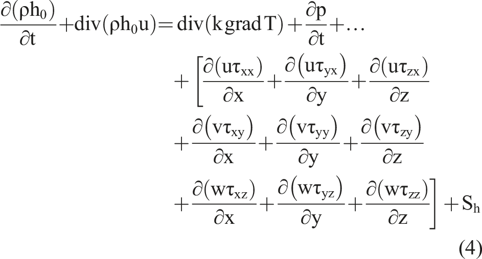
Turbulence modeling
Flow interactions between rotating and stationary blades are known as the dominant source of unsteadiness and periodic flows in a gas turbine engine. Following research works of Johansson et al.,
32
Bosch and Rodi,
33
and Tatsumi et al.,
34
the equations are presented in a form that mainly reflects this potentially periodic flow nature.
1
By averaging the Navier–Stokes equations, the URANS equations can be obtained as follows: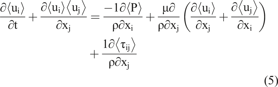
The role of a turbulence model is to approximate the Reynolds stress terms, which is defined as the following relation.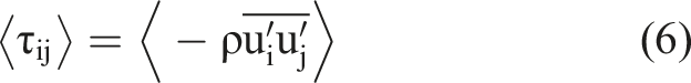
Generally, the well-known Boussinesq approximation is used to evaluate this parameter as follows: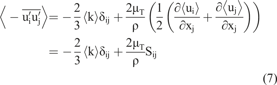
In which
LES equations
In the large eddy simulation (LES) method, spatially filtered variables (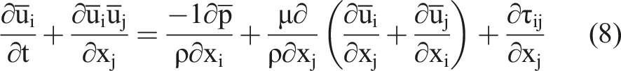
Also, 
The first term on the right hand side of the above equation is the usual Reynolds stress. The last two components, called the Leonard (
Hybrid method of RANS-LES (DES)
Applying LES technique for boundary layer problems with high Reynolds numbers is prohibitively time consuming and expensive. Therefore, using this method is usually not recommended for simulation of many practical problems. 36 On the other hand, turbulent structures can be resolved in massively separated regions, where large turbulent scales are of the same dimensions as the geometrical structures (like airfoil flaps, buildings, and blunt trailing edge turbine blades). Detached Eddy Simulation (DES) is an attempt to combine elements of URANS and LES formulations to achieve a hybrid formulation, where URANS is used inside the attached and mildly separated boundary layers and LES is applied in massively separated regions.
In the present research work, the DES technique based on the SST formulation is utilized for the solution of the flow field. The SST model supports the formulation of Zonal DES formulation, 37 which is less sensitive to the grid resolution restrictions than the standard DES formulation, as proposed by Strelets 38 (refer to the ANSYS CFX technical report 39 for more details).
Strelets formulation for SST-DES
The idea behind the Strelets DES model
38
is to switch from SST-URANS model to the LES model in regions where the turbulent length (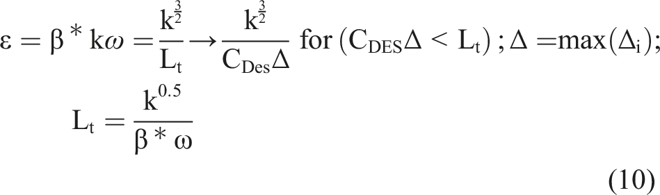
Practical reason for choosing maximum edge length (as a safest estimate) in the DES formulation is that the model must be returned to the RANS formulation in the attached boundary layers. The modified DES by Strelets can be formulated as a multiplier to destruction term in the k-equation, as follows: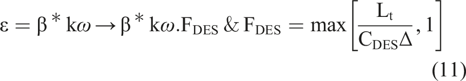
The numerical formulation is also switched between an upwind biased and a central difference scheme in the RANS and DES regions, respectively.
Zonal SST-DES formulation in CFX
The main undesirable problem in DES formulation (in both the Spalart–Allmaras and the standard SST-DES models) is a type of flow separation which is lunched in the regions where the local surface grid spacing is less than the boundary layer thickness (i.e., 
One can refer to the ANSYS CFX technical report 39 for more details.
Mesh generation
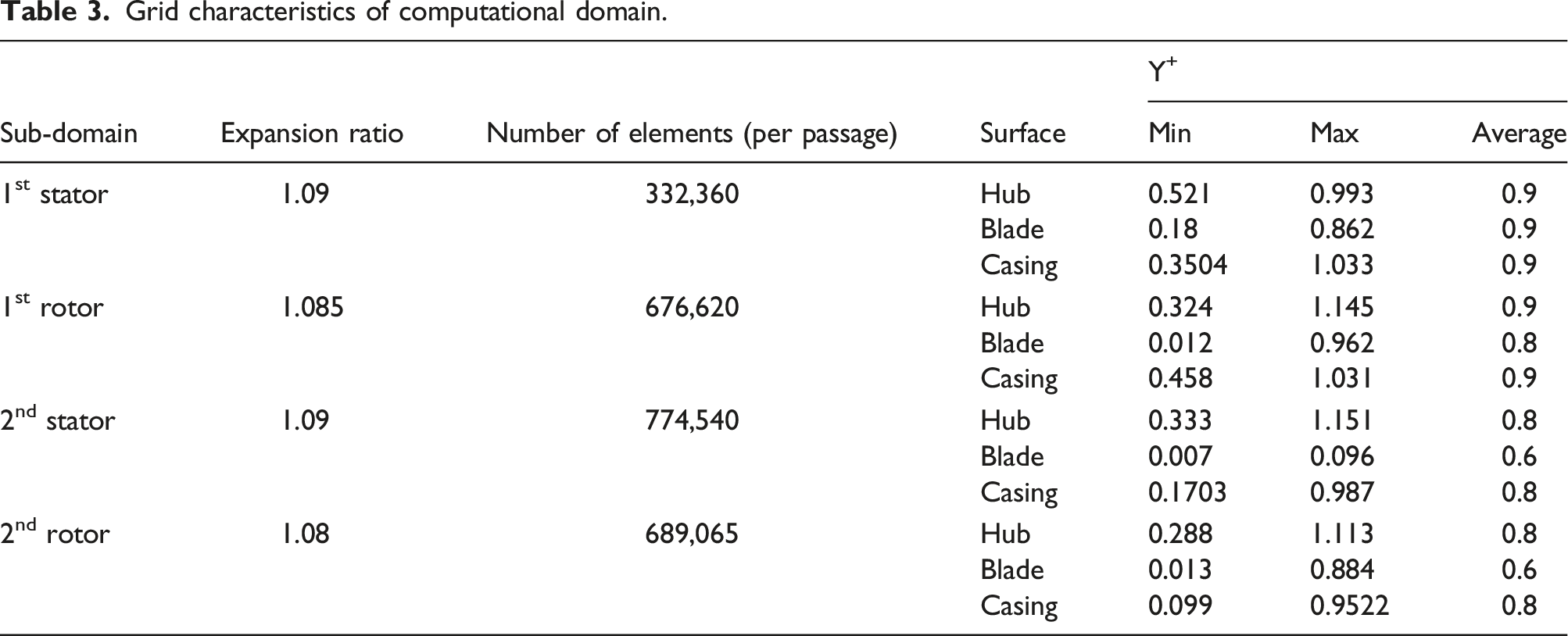
Grid characteristics of computational domain.
Mesh structure on the blades surfaces, inlet boundary, and hub is shown in Figure 5 for each sub-domain. Fine meshes are distributed for the regions of high sensitivity, such as the blades leading and trailing edges regions. Grids distributions on blades surfaces along with detail view of sensitive regions.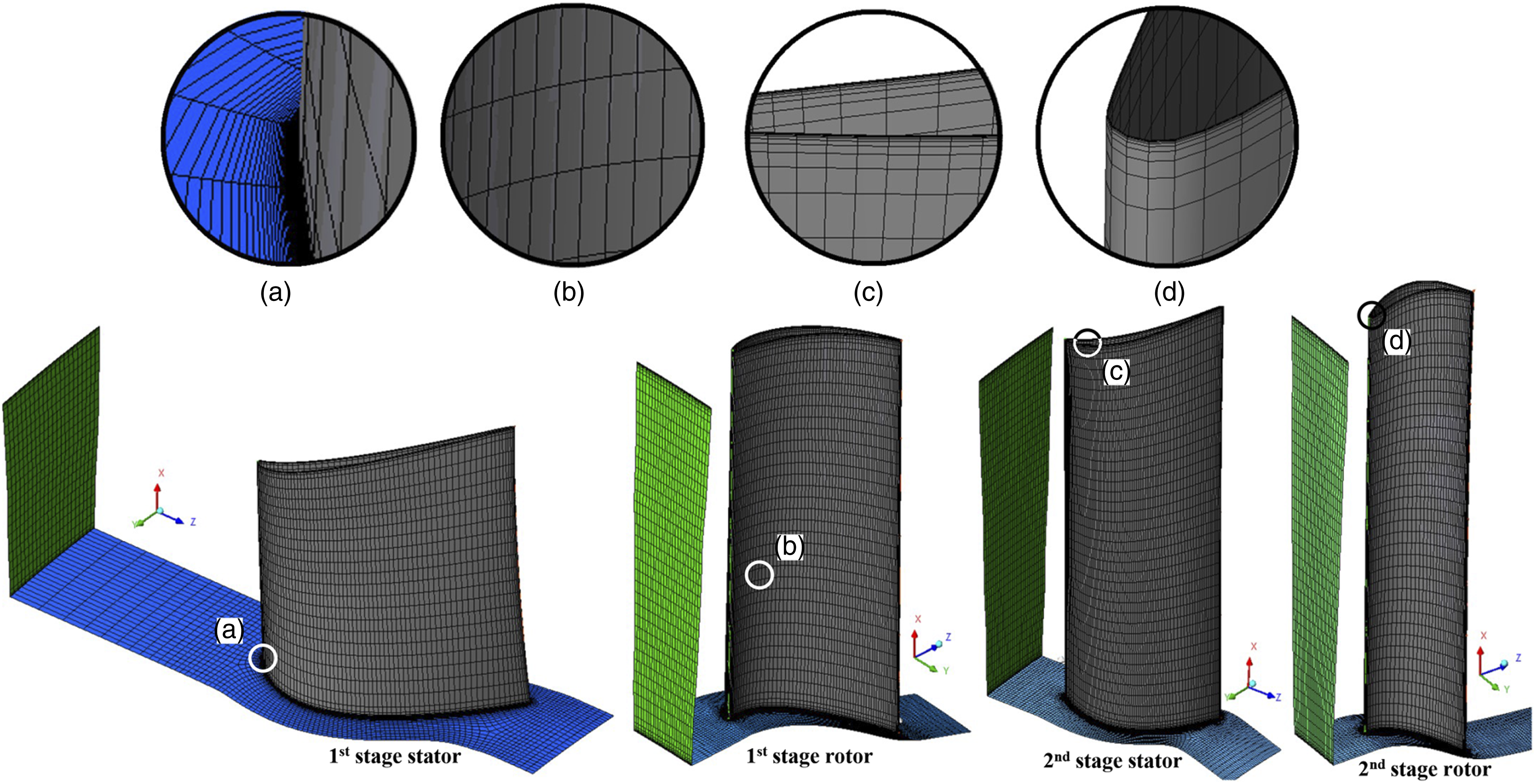
The total number of elements is equal to about 8.5 million. This number of elements has been selected as a result of examining the independency of results to the number of grids. Figure 6 is related to mesh independency studies, which shows the variations of the total-to-total efficiency against the number of elements. Variations of total-to-total efficiency with number of meshes.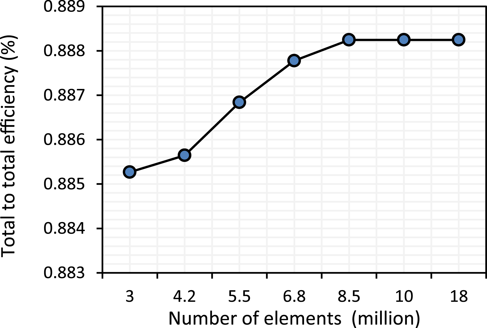
Y+ contours for the stator and rotor blades of the second stage are shown in Figure 7. Due to implementation of Y+ plus contour on second stage components.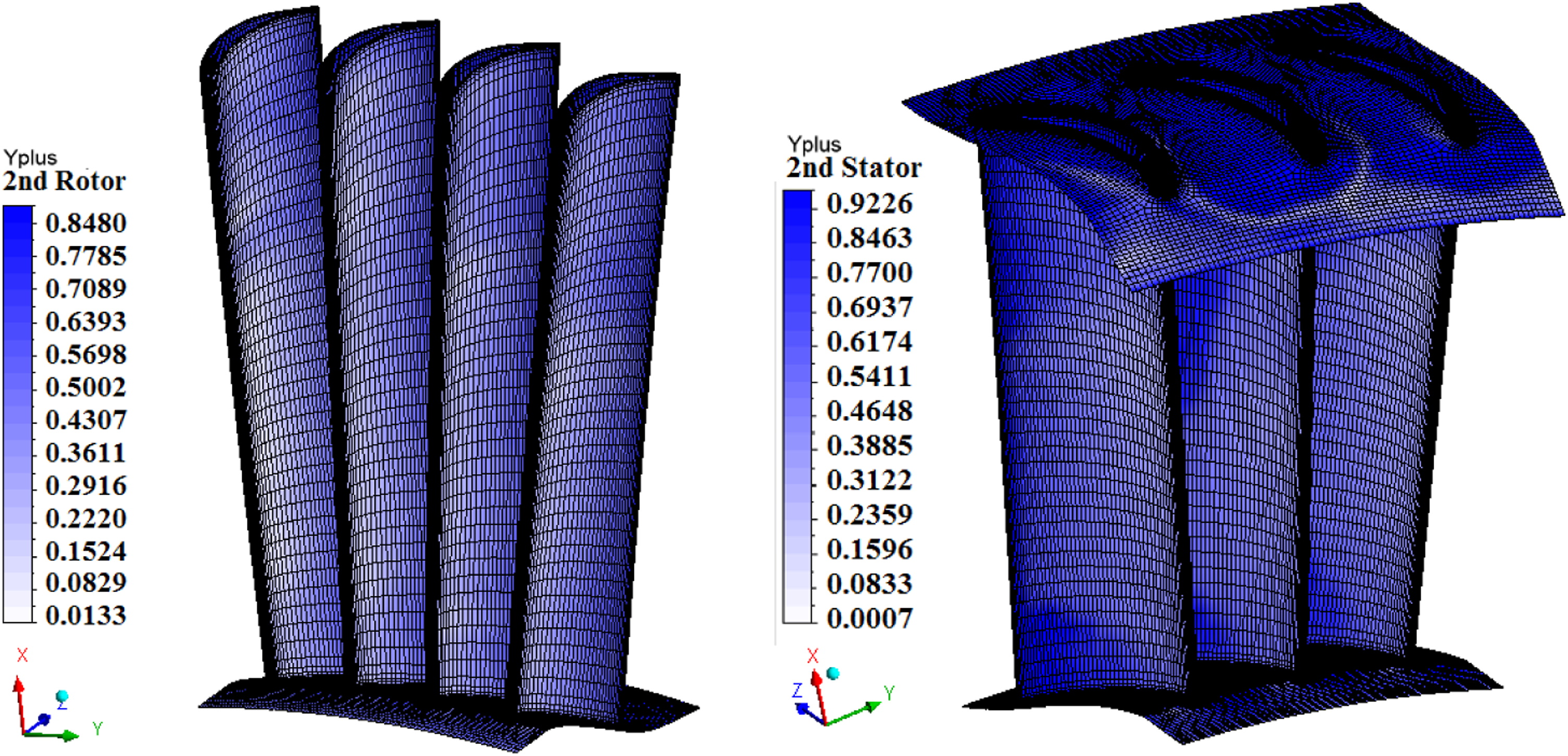
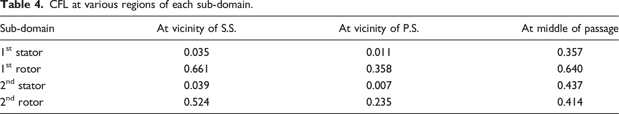
CFL at various regions of each sub-domain.
Results
It is obvious that the flow within the turbine is inherently unsteady. However, steady simulations can provide a general view of the governed flow field properties, at the initial level of the analyses. Steady simulations enabled the present authors to obtain the worst and the optimum clocking positions, among the five clocking positions already introduced in Figure 4. Considering the turbine efficiency as the main target through the optimization process, the worst and optimum cases were recognized as CLP1 and CLP4, respectively (see Figure 4). Then, unsteady analyses have been carried out to study the clocking effects of the second stator blades on the flow structure and the general performance of the turbine for these two cases. Based on Bohn conclusion, steady analyses would be sufficient to attain the worst and optimum clocking positions.13,15
Wake deformation within blades passage
To demonstrate the wake deformation, results of instantaneous entropy and turbulent kinetic energy distributions on an imaginary mid-span plane of the second rotor blades row are presented in Figure 8. Five normalized time steps (t/τ = 0 to 1 with 0.25 s intervals) are considered for presentation of the results. τ is the wake passing time through the second rotor blades passage. Instantaneous contours of entropy (parts: “a” to “e”) and turbulent kinetic energy (parts: “f” to “j”) on second rotor blades mid-span plane.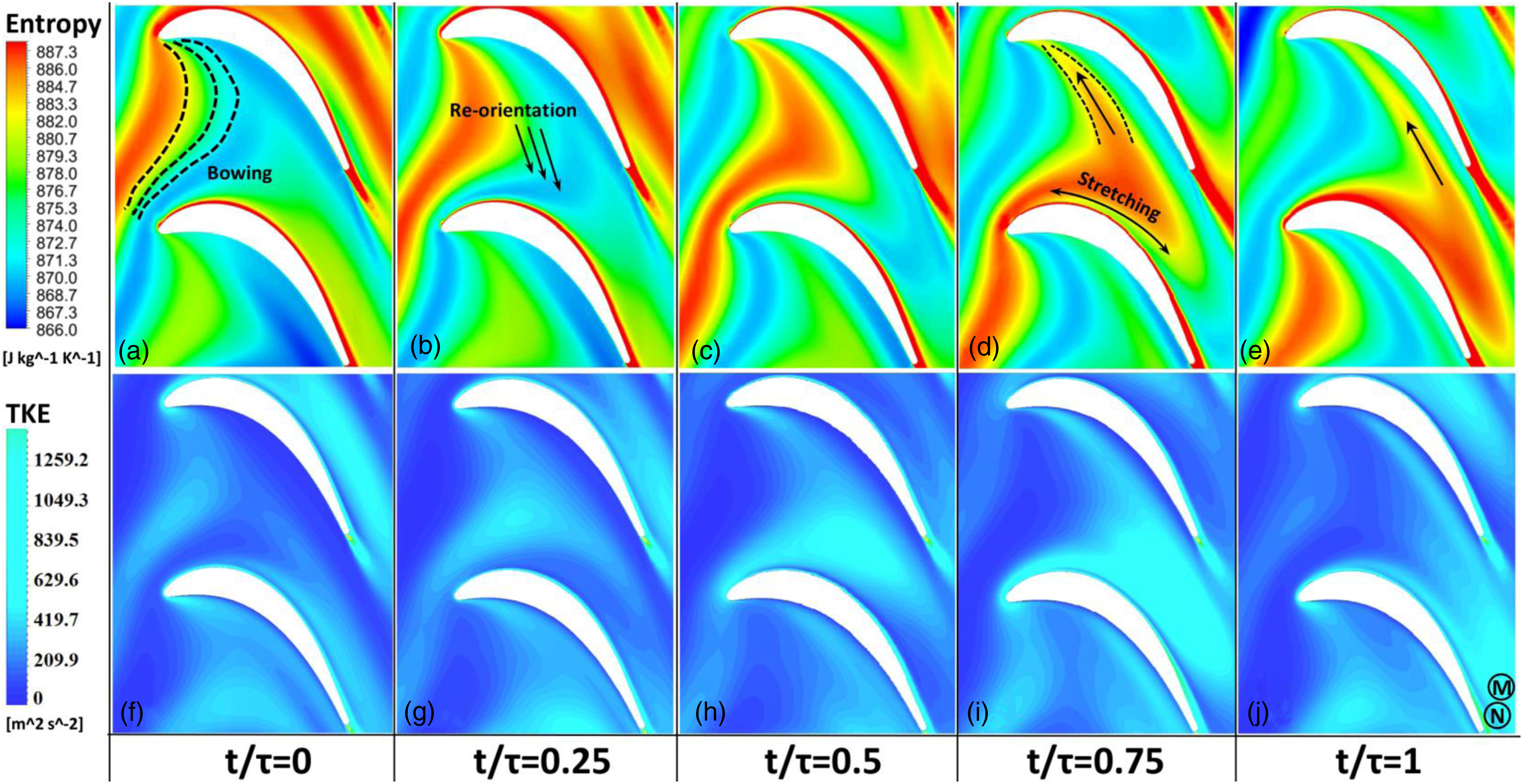
Based on Smith’s investigations, the moving wake segment through the blades passage includes specific movements of V-shape motion, re-orientation, elongation, and expansion/stretching. 41 V-shape motion (or bowing) of the wake occurs near the blade leading edge, where the local velocities in the middle of the passage are higher than those near the blades solid surfaces. This type of movement is shown in Figure 8(a)–(c). The velocities near the suction side are higher than those near the pressure side which results in re-orientation of the wake segment due to rapid convection of the wake near the suction side.
Stretching occurs when the first part of the wake reaches the blades leading edge region. While moving downstream, this process accelerates on the blade suction side. Based on the results presented in Figure 8(c)–8(e), the wake width has increased on the blade suction side as a result of stretching. Differences in local convection velocities along the passage result in wake elongation wake. This process makes a narrow tail of the wake flow towards the blade pressure side (shown by arrow sign in Figure 8(d) and 8(e)).
Contours of entropy and turbulence intensity at the second rotor blades mid-span are shown in Figures 9 and 10, respectively. To get manifest rotating areas, operator of curl is applied on the velocity vectors in a three-dimensional space. The result would obviously be the vorticity vectors. Projection of this vorticity field on the mid-span surface (as a 2-D plane) would produce lines which are superimposed in Figure 9. There can be seen a clear concentrated lines of this type at the wake leading edge region; indicating existence of highly rotational flow. Entropy contour at 2nd rotor mid-span. Turbulence intensity contour at 2nd rotor mid-span.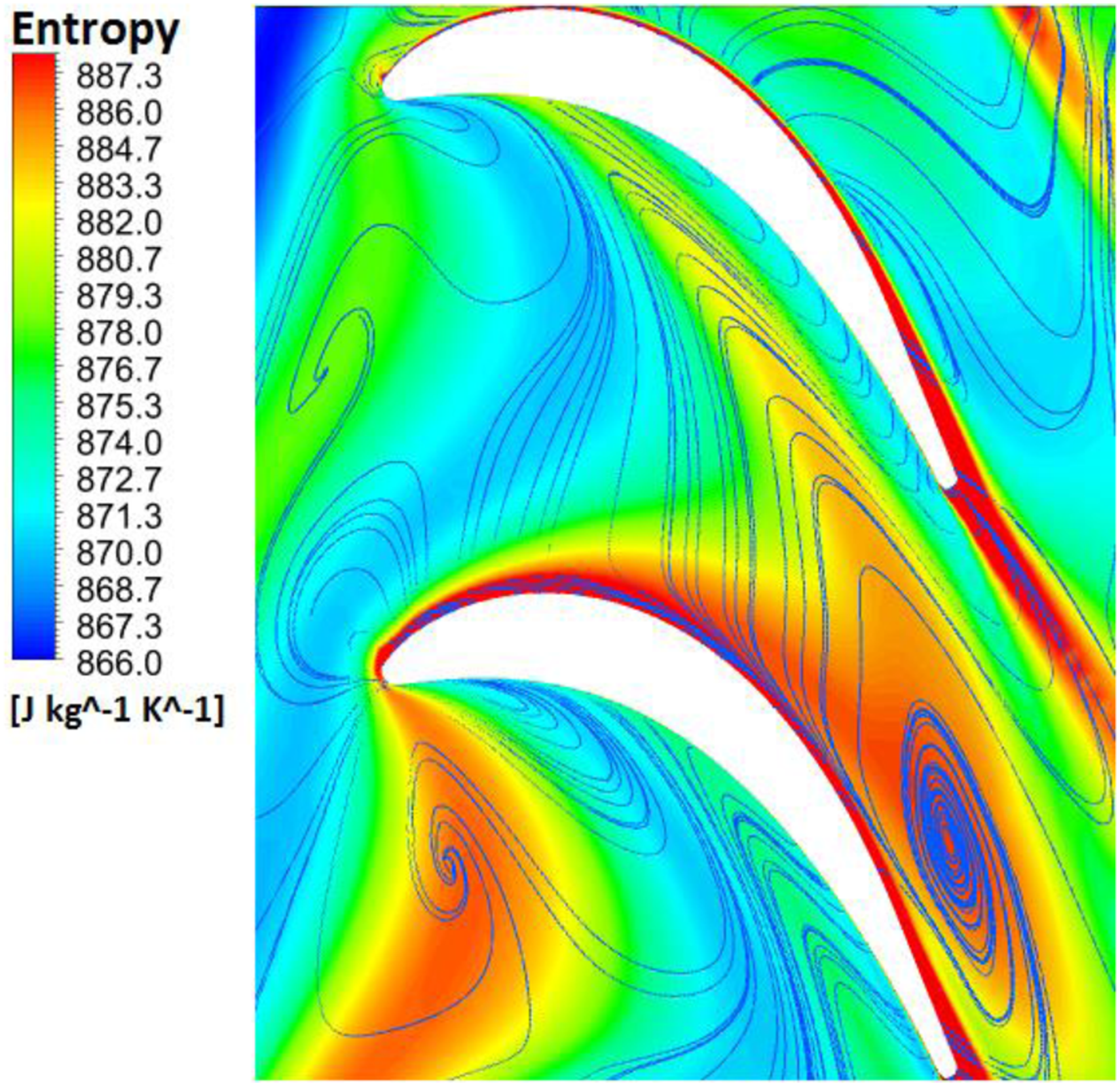
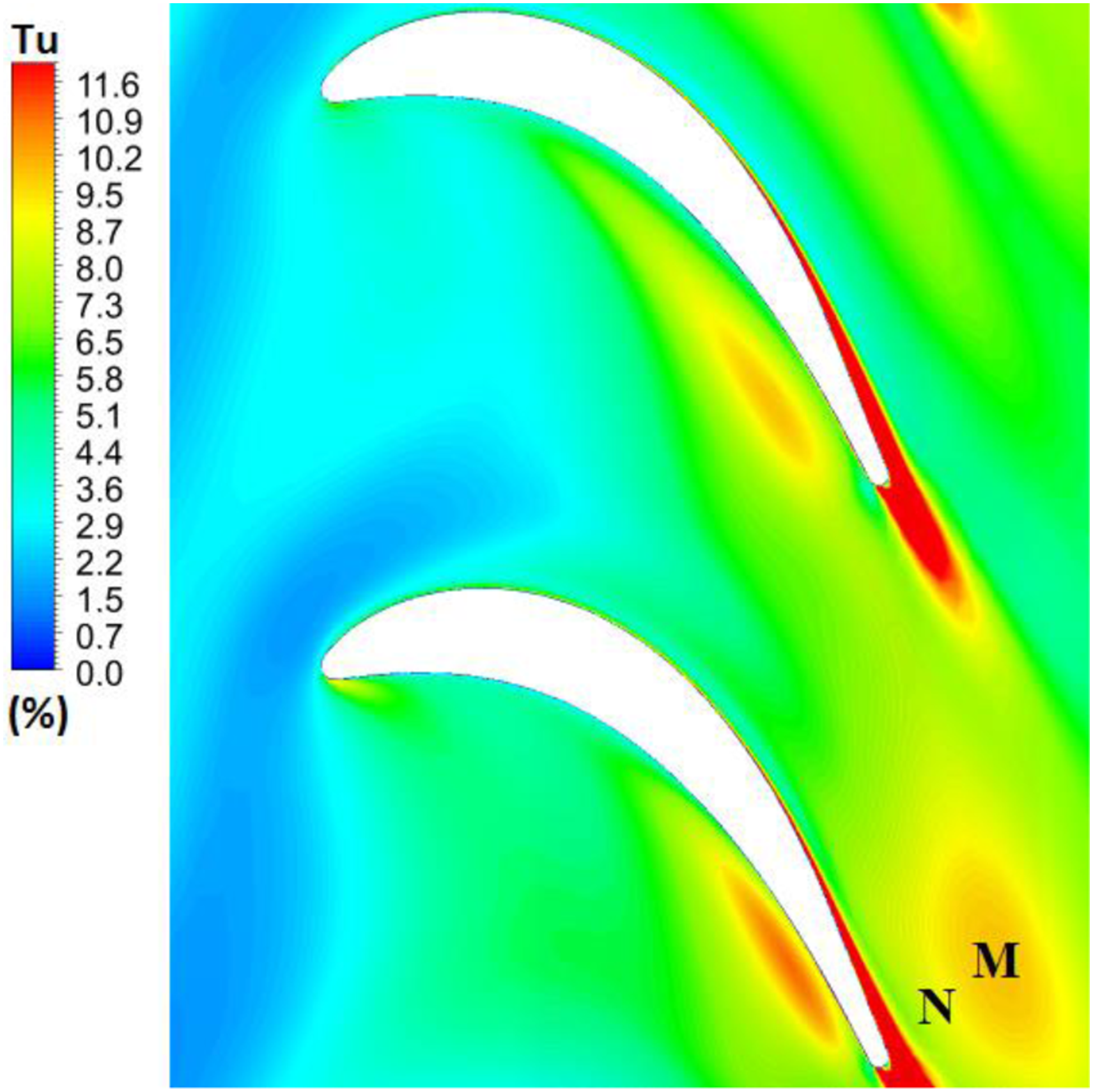
The highest level of TKE is taken place outside of boundary layer as designated by capital letters of M and N in Figure 8(j). The rich TKE regions indicate locations in which core of the wake flow accumulates near the blade suction side. Referring to Figure 10, the Tu value at the center (region M) and the leading edge, the wake flow (region N) is about 9% and 8%, respectively. Similar observations have been presented by Michelassi et al. based on DNS and LES methods through their numerical simulations of the blade-wake interaction. 42
Flow topology at second stator inlet
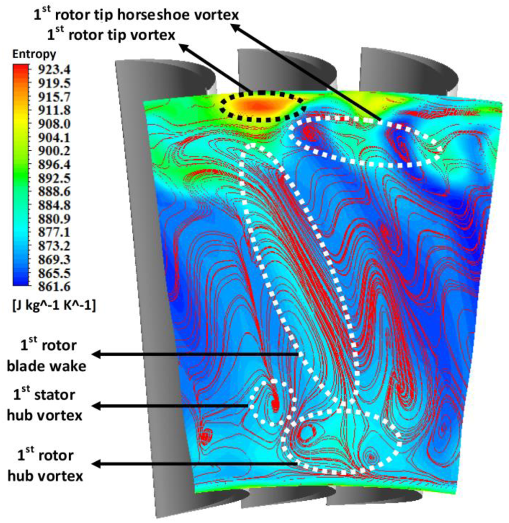
Flow structures around the second stator blades are shown in Figure 11. These results are presented by Q-criterion, for visualization of core region of the vortical flows. The Q-criterion, reflecting both the vorticity and strain rate of the fluid elements,
43
is attributed to relative dominance of the rotational component over the stretching component in deformation of a fluid element. With regard to Figure 11, various types of vortices, originating from the upstream, can be recognized. Figure 12 shows entropy contour at the second stator inlet. In addition, rotating areas are visualized by applying operator of curl on the velocity vectors (i.e., superimposed red lines) which represent the core of prominent rotational areas (i.e., center of strong vortices). Flow topology at second stator inlet. Entropy contour at second stator inlet.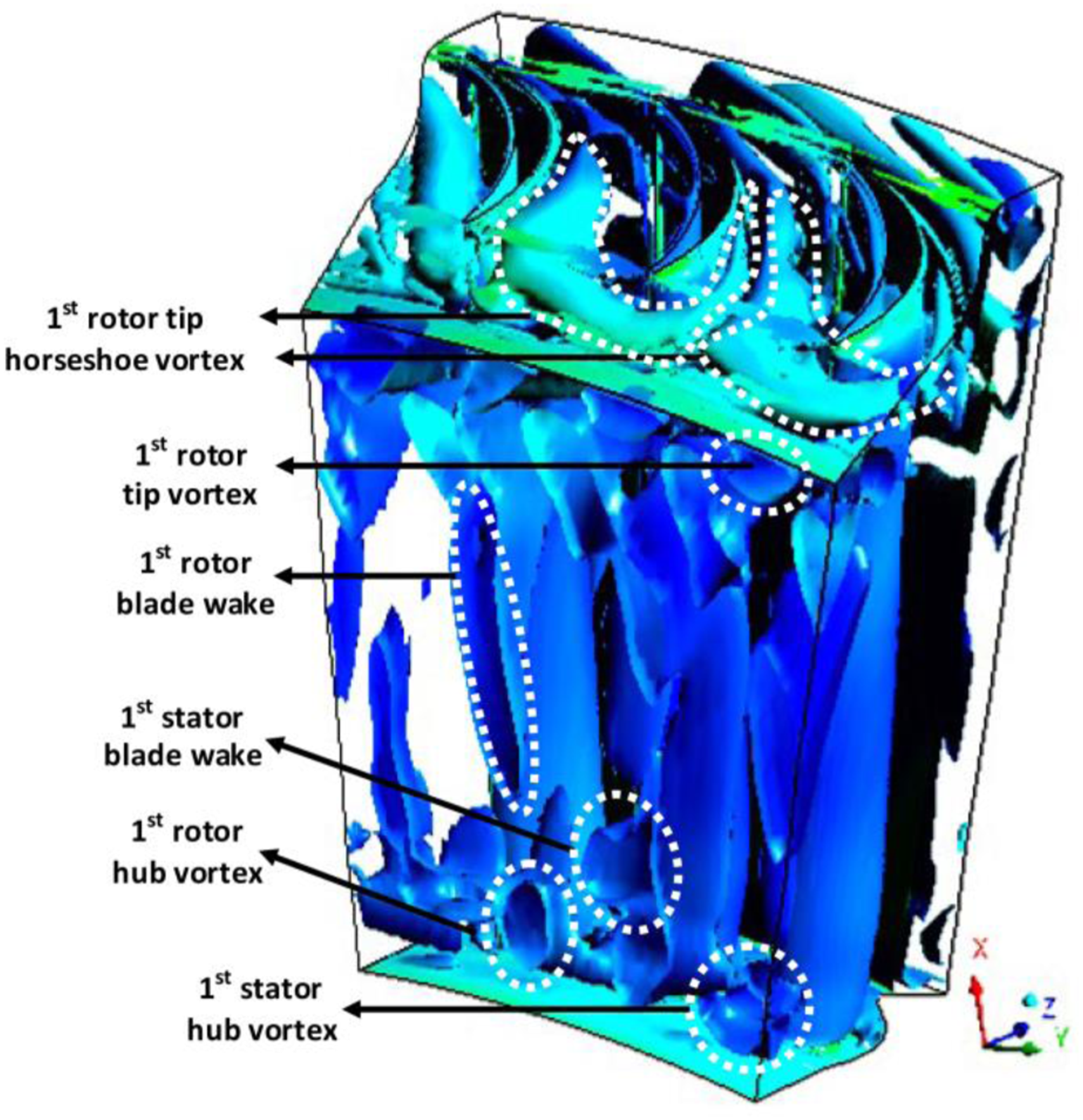
Transient wake effect on blade loading
Wake deformation in the second stator blades passage is presented in Figure 13 in terms of instantaneous entropy contours on an imaginary mid-span plane. Wake deformation within the blades passage is already introduced in the Wake deformation within blades passage section for the rotor blades. As shown in Figure 13, the same deformations are also occurred within the stator blades passage. Out of 15 normalized time steps, started from t/τ = 0 to 1 with equal intervals, five time steps are selected for presentation and discussion. Instantaneous entropy contour on second stator blades mid-span. (a) t/τ = 0, (b) t/τ = 0.214, (c) t/τ = 0.285, (d) t/τ = 0.714, (e) t/τ = 1.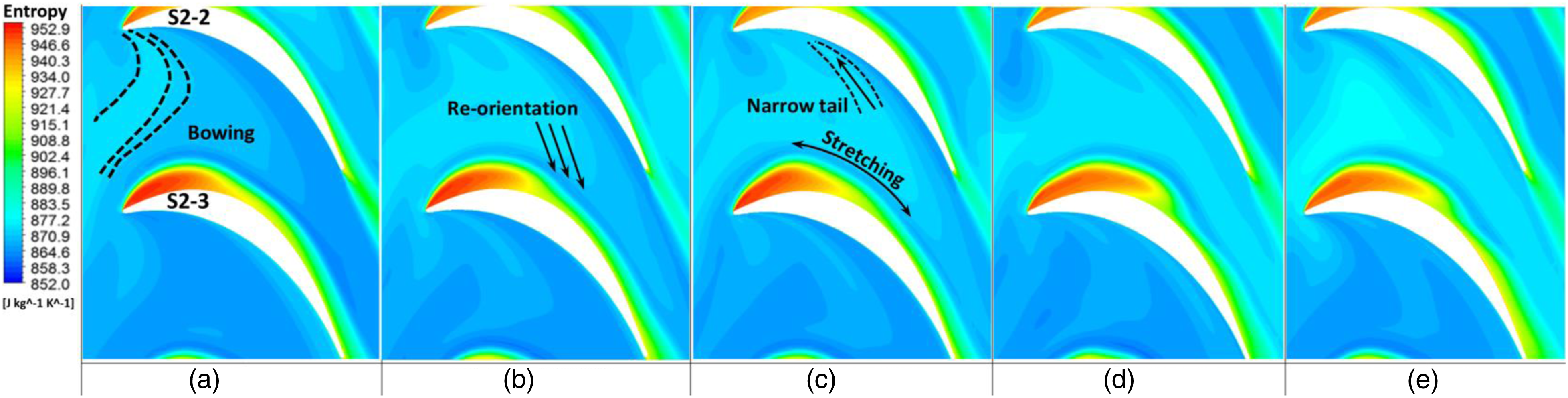
Results of instantaneous blade loading (CL) and minimum pressure coefficient (Cp, min) on the second stator (S2-2) at its mid-span are presented in Figure 14 for 15 subsequent normalized times. Results of executing URANS are also superimposed in this figure for comparison with those obtained through DES. Cp, min is representative of the maximum velocity, which can cause dominant effect on the lift force (the more suction, the more blade loading). Obviously, Cp, min and CL must mostly obey the same trend of variations. Time-dependent aerodynamic parameters of S2-2 blade.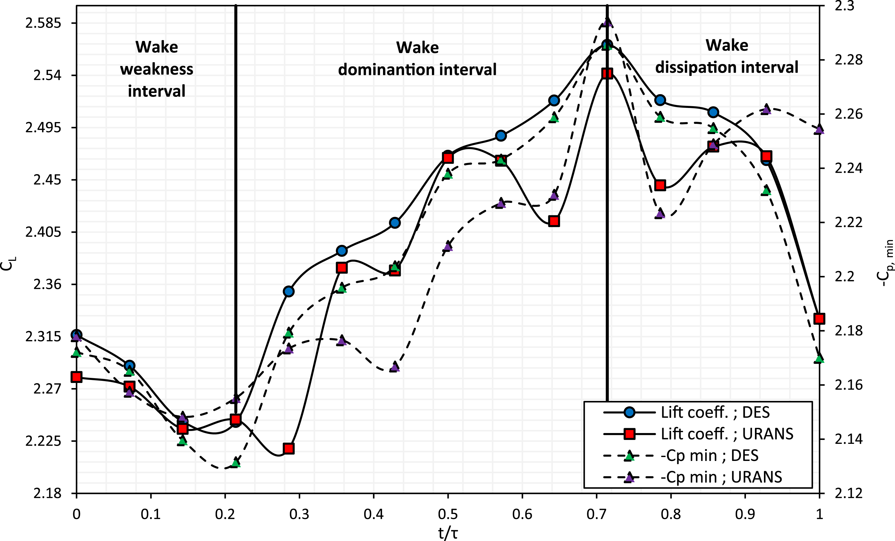
Within the time interval of t/τ = 0 to 0.214, −Cp, min and CL are decreasing with low slops either using DES or URANS. So it can be concluded that the leading part of the wake is not so strong in this time interval. This situation is designated by “wake weakness” in Figure 14 (see also Figure 13(a) and (b)). Then, beyond t/τ = 0.214, both the DES and URANS show that the parameters −Cp, min and CL are increasing up to their peak values at t/τ = 0.714. This time interval is designated by “wake domination” in Figure 14 (see also Figure 13(c) and (d)). This interval can be justified by re-orientation process which leads to a negative jet toward the suction side which causes the velocity to increase (or pressure to decrease) on the blade suction side. 44 Referring to Figure 14, it can be seen that using URANS produces oscillatory results in comparison to those of DES, which is not consistent with what would be expected. 44 In addition, there are some instances in which Cp, min and CL behave opposite each other (in URANS), which is not reasonable.
Results of Cp, min and CL reasonably show the same trend of continuous reduction within t/τ = 0.714 to 1 while executing DES. This time interval is designated by “wake dissipation” in Figure 14 (see also Figure 13(e)), since both the Cp, min and CL are decreasing. Applying URANS has produced again oscillatory results. In addition, Cp, min and CL behave opposite each other in some instances (in URANS), which is not reasonable.
Generally speaking, it can be deduced that the DES results show a logical relation between variations of CL and Cp. This superiority is the main reason of choosing DES turbulence modeling in this research work instead of URANS.
Clocking effects on performance
It would be worthy to use total-to-total efficiency (
Time-averaged results of rotor blades rows.
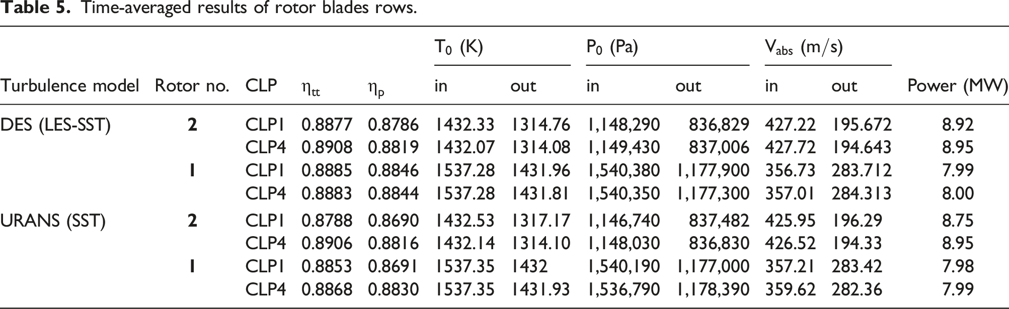
Based on results obtained by DES turbulence modeling, it can be deduced from this table the
Although the first stator is fixed and clocking is enforced on the second stator blades, the first stage output power can be altered under clocking. This is due to the nature of the governing subsonic flow, which causes any disturbance to propagate all through the flow field. Referring to DES results in Table 5, it can be deduced that in CLP4 case, the first rotor output power has increased by 0.125% in comparison to CLP1. Therefore, the output power of the whole two stages in CLP4 has increased by 0.237% in comparison to CLP1.
Performance analysis of second stator blades
As already mentioned, the CLP4 and CLP1 are recognized as the optimum and worst cases, respectively. Figure 15 shows positions of the one rotor blade of the second stage at five successive normalized times. Results of the time-dependent flow properties of the second stator blades are shown in Figure 16. Mid-span position of one rotor blade of second stage at five normalized times. Time-dependent properties of second stator blades.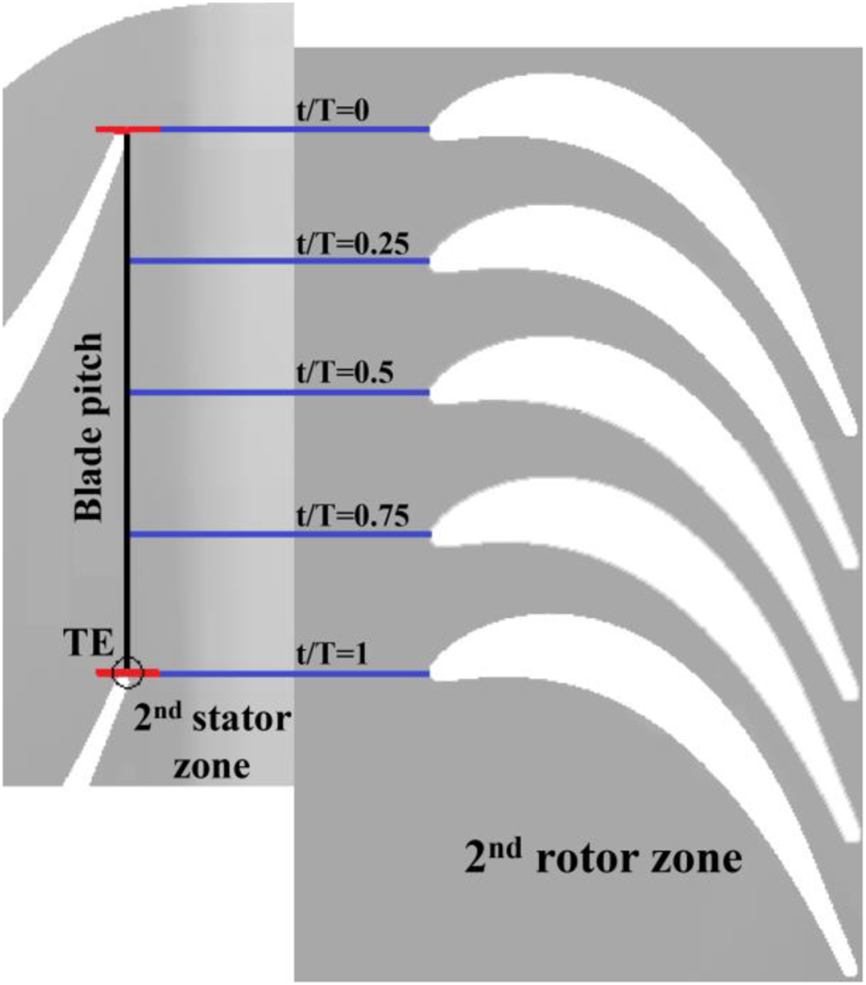
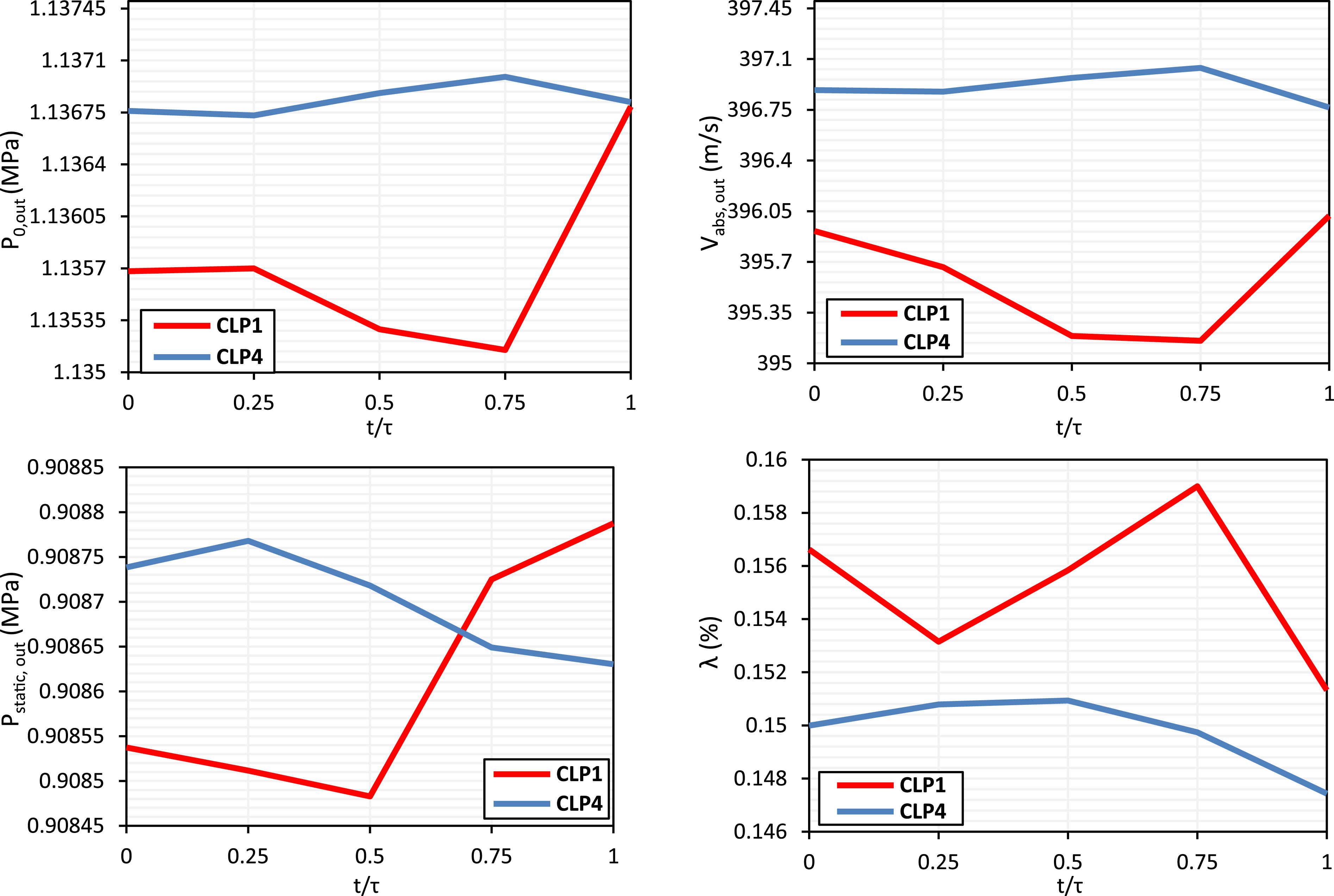
It can be observed that outlet velocities in CLP4 is always higher than those in CLP1, which results in higher outlet total pressure in the former case. As expected, CLP4 is accompanied by the lowest pressure loss coefficient.
Blade-wake interaction under clocking
Trajectory of the wake flow within the blades passages of the second stage, basically originated from the first rotor blades row, is presented and discussed in this section for the CLP1 and CLP4 cases in terms of the instantaneous entropy contours. Results of mid-span are presented in Figure 17 for five subsequent normalized times. The inlet boundary condition is the same for all the clocking positions. In addition, no significant event has been observed within the first stator blades while imposing the clocking on the second stator. Therefore, the contours shown in Figure 17 run from the first rotor. Instantaneous entropy contour at mid-span.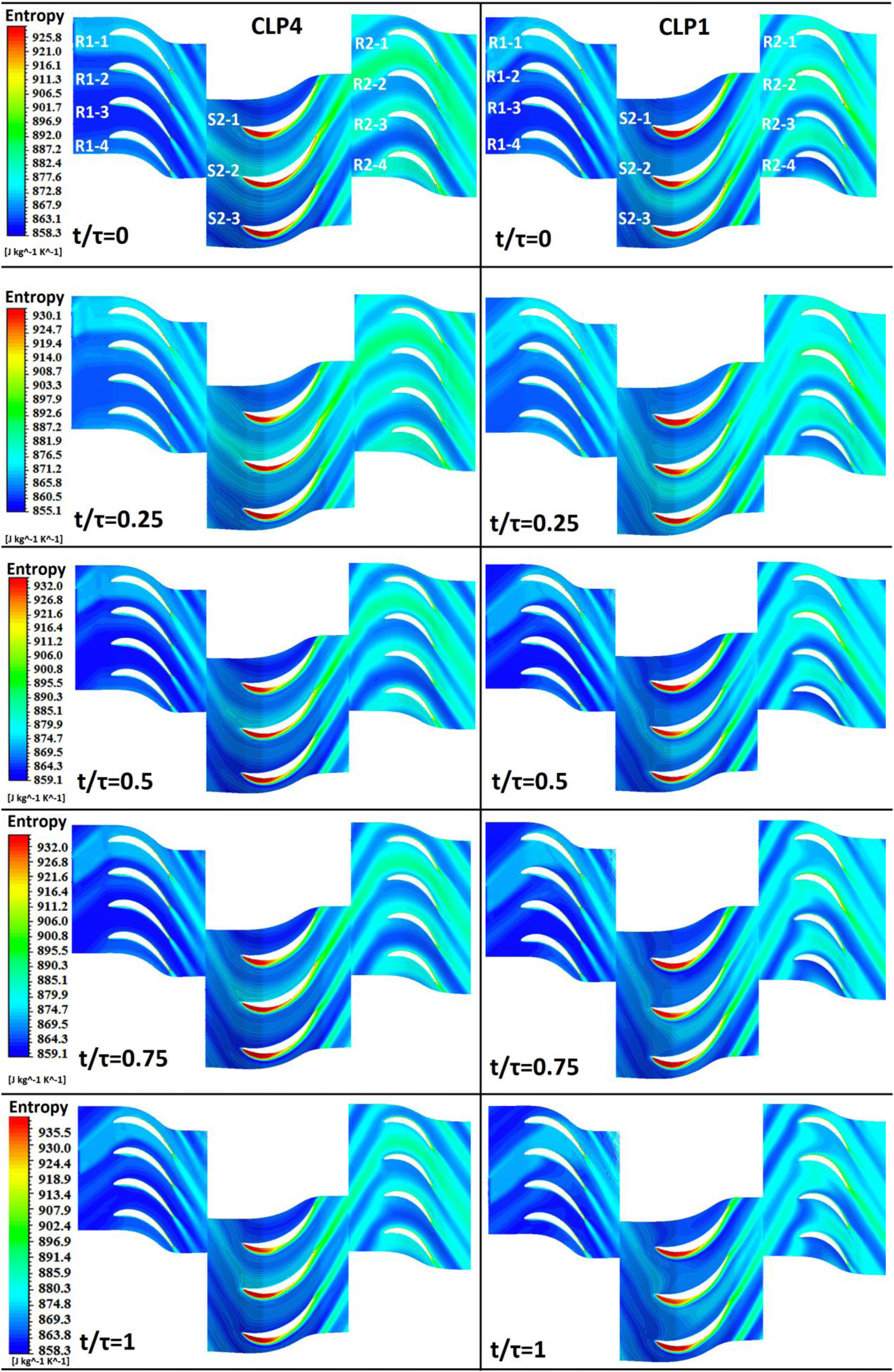
Stator blade-wake interaction
In CLP4 case, a strong wake impinges on S2-2 leading edge mostly leaning toward the pressure side, within the whole duration. But in CLP1, a strong wake passes the middle space of the passage between S2-2 and S2-3 blades from t/T = 0 to 0.25. This type of wake trajectory causes pressure loss to increase for CLP1 in comparison to CLP4 (see Figure 16 and time-averaged results in Table 5). With time advancing from 0.25, a significant part of a wake hits S2-2 leading edge and enters the passage between S2-2 and S2-3 blades in CPL1 case, which causes lower outlet total pressure of the second stator in comparison to CLP4.
Rotor blade-wake interaction
Regarding Figure 17, at t/T = 0 in CLP4 case, a strong wake has entered the passage between R2-1 and R2-2 blades mildly hitting their leading edges. With time advancing, the above-mentioned wake moves towards the R2-2 and impinges on its leading edge. Ultimately, at t/T = 1, it is cut-off by R2-2 blade due to its rotational movement. At t/T = 0, the wake flow is swept all over the R2-3 suction side and R2-4 is fully covered by another wake. With time advancing, the wake sweeping R2-3 suction side becomes weaker as it moves downstream.
At t/T = 0 in CLP1, R2-1 suction side is completely swept by a wake and R2-2 is completely covered by another one. With time advancing, the wake covering R2-1 becomes weaker and is cut-off due to rotational movement of the blade. At t/T = 1, it is placed at inlet of passage between R2-1 and R2-2. There is a similarity in CLP4 case at t/T = 1 for the wake impinging the R2-3 leading edge.
With time advancing in CLP1 case, the wake covering R2-2 gradually becomes weaker while moving downstream, as R2-2 exits the wake area. But finally, the above-mentioned wake is cut-off by R2-3 and at t/T = 1 and enters the passage between R2-2 and R2-3. It can be seen that at t/T = 0 in CLP1 case, a strong wake passes through the middle space of the passage between blades R2-3 and R2-4 without hitting the leading edges. This process is accompanied by strong losses, which in turn, causes the blade loading to decrease. With time advancing until t/T = 1, this wake is almost completely interrupted by R2-4.
Unsteady aerodynamic of second stator blades
Figure 18 illustrates instantaneous entropy contour on the second stator blades row inlet boundary for two cases of CLP4 and CLP1 at three succeeding normalized times. It can be distinguished that at t/T = 0 in CLP4, a continuous wake segment formed from the blade hub up to around the mid-span impinges on the S2-2 leading edge. As already mentioned, this situation causes the blade loading to increase and the losses to decrease. But at the same time, for CLP1 case, a strong wake, from hub to around 80% span, enters the passage between S2-2 and S2-3. Hence, in CLP4 case, it is expected that in this interval, outlet total pressure is increased. In both of the CLPs, the wake becomes weaker with passing time. Instantaneous entropy contours at second stator inlet boundary.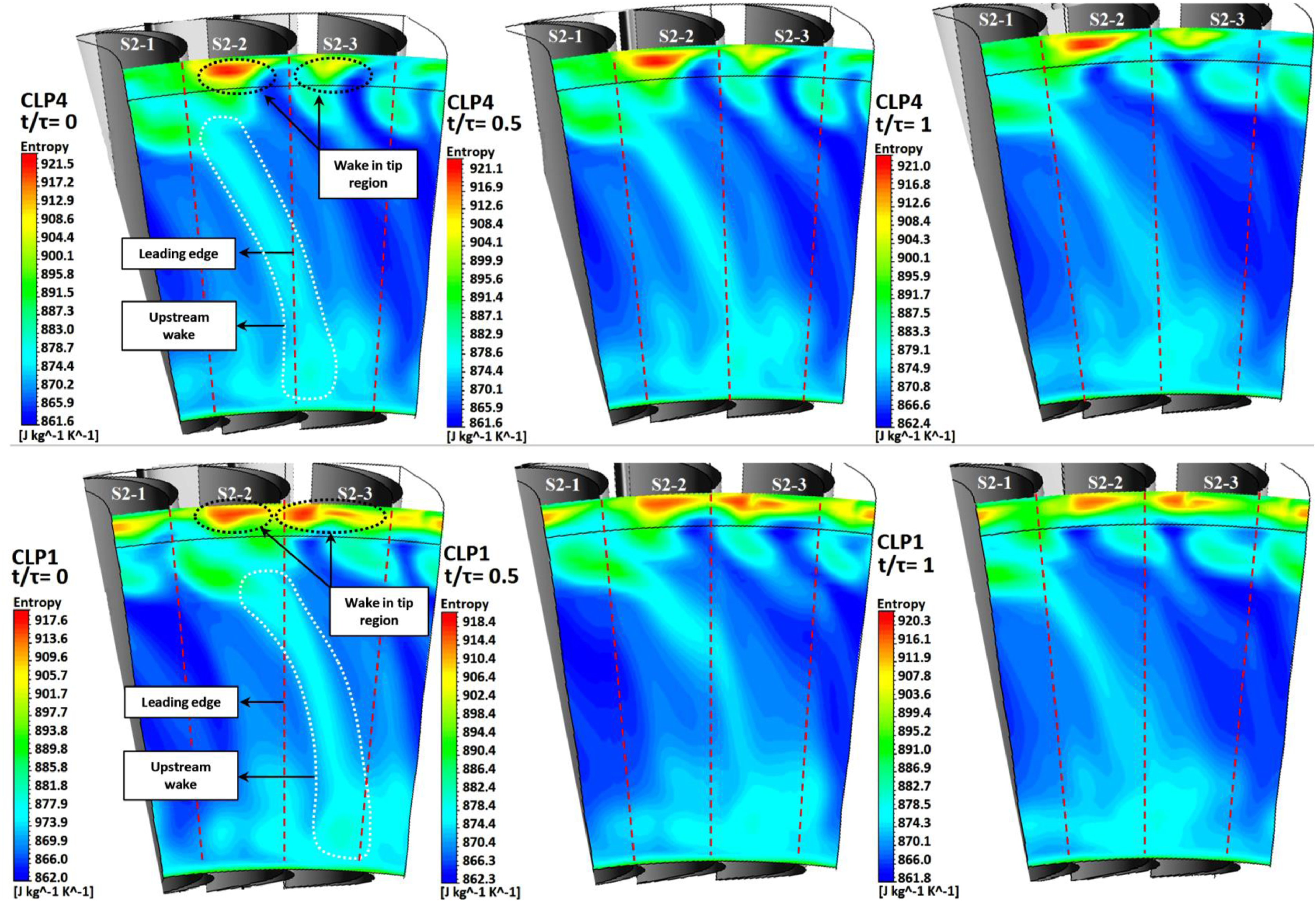
In CLP4 case at t/T = 0, there is a strong wake entering the passage between S2-1 and S2-2 near the blades tip, which moves towards the S2-2 leading edge with time advancing. In contrast to CLP1 case, at the same time, two strong wakes enters the passage between S2-1 and S2-2 and the passage between S2-2 and S2-3. Therefore, it can be concluded that CLP4 shows a better aerodynamic performance (consistence with higher total pressure) in comparison to CLP1 case, within the hub to near the mid-span and also around the tip outlet.
Figure 19 shows instantaneous total pressure contour on the second stator outlet boundary for two cases of CLP4 and CLP1 at three normalized time. High-pressure regions at second stator outlet in CLP1 case exclusively are established around 70% span up to the tip at the middle of boundary. But in CLP4 case, flow between stator blades has more pressure. This superiority is attributed to the entry situation of the wake at the second stator inlet and can be justified from Figures 17 and 18. Variations trend of outlet total pressure in each region can be estimated with regard to the wake entry situation, whether it impinges on the leading edge or enters the blades passage. Instantaneous total pressure contours at second stator outlet boundary.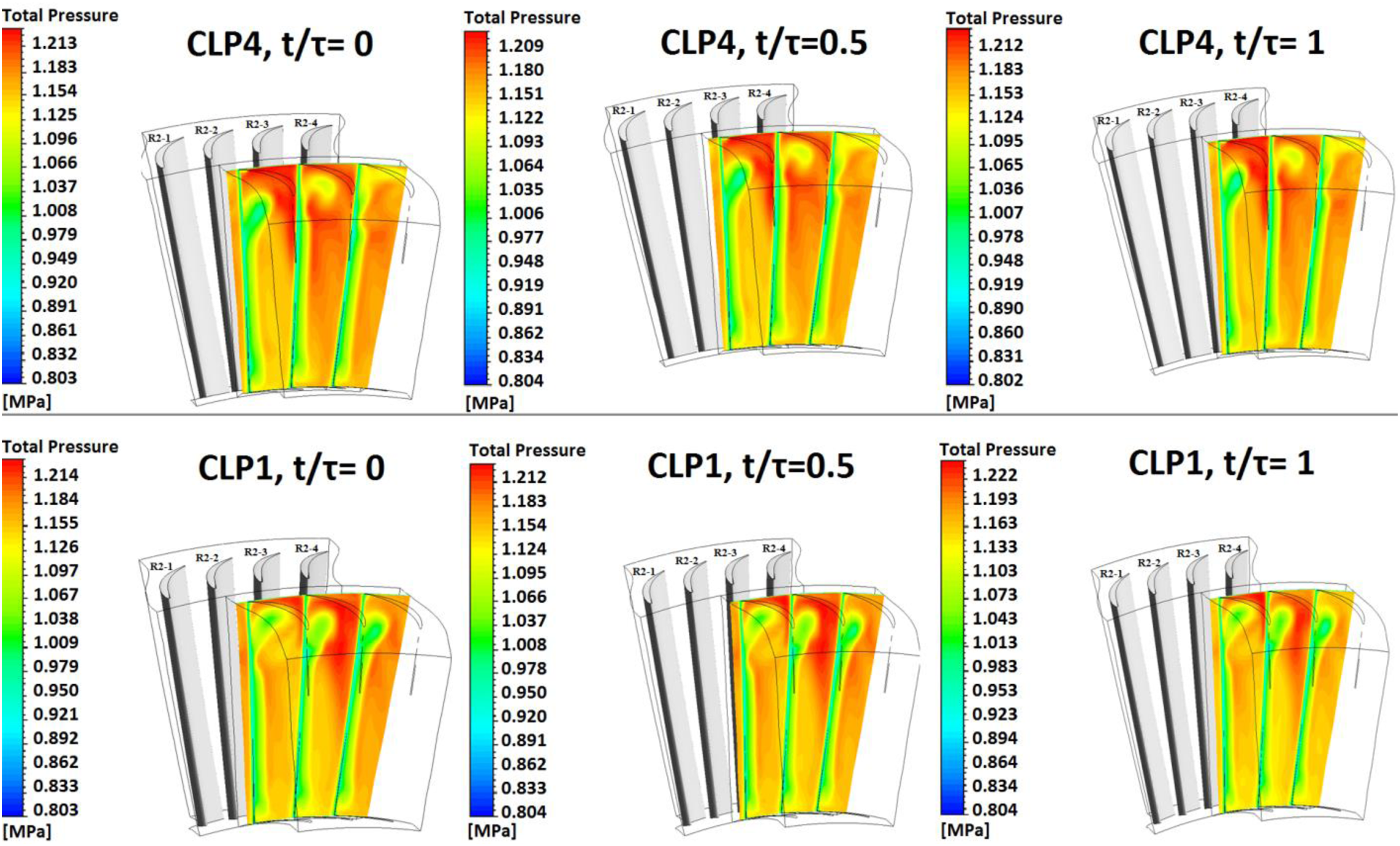
Aerodynamic performance of second stator at a snap shot
Figure 20 presents spanwise variations of the second stator outlet pressure, velocity, and pressure loss coefficient at t/T = 0.5 for two cases of CLP4 and CLP1. It can be seen that around 80% span up to the blades tip region, stator outlet total pressure in CLP4 case has significantly increased in comparison to CLP1 case. Undoubtedly, variations in total pressure can be justified with wake entry situation according to the instantaneous contours in Figures 18 and 19. Spanwise flow properties of second stator at t/T = 0.5.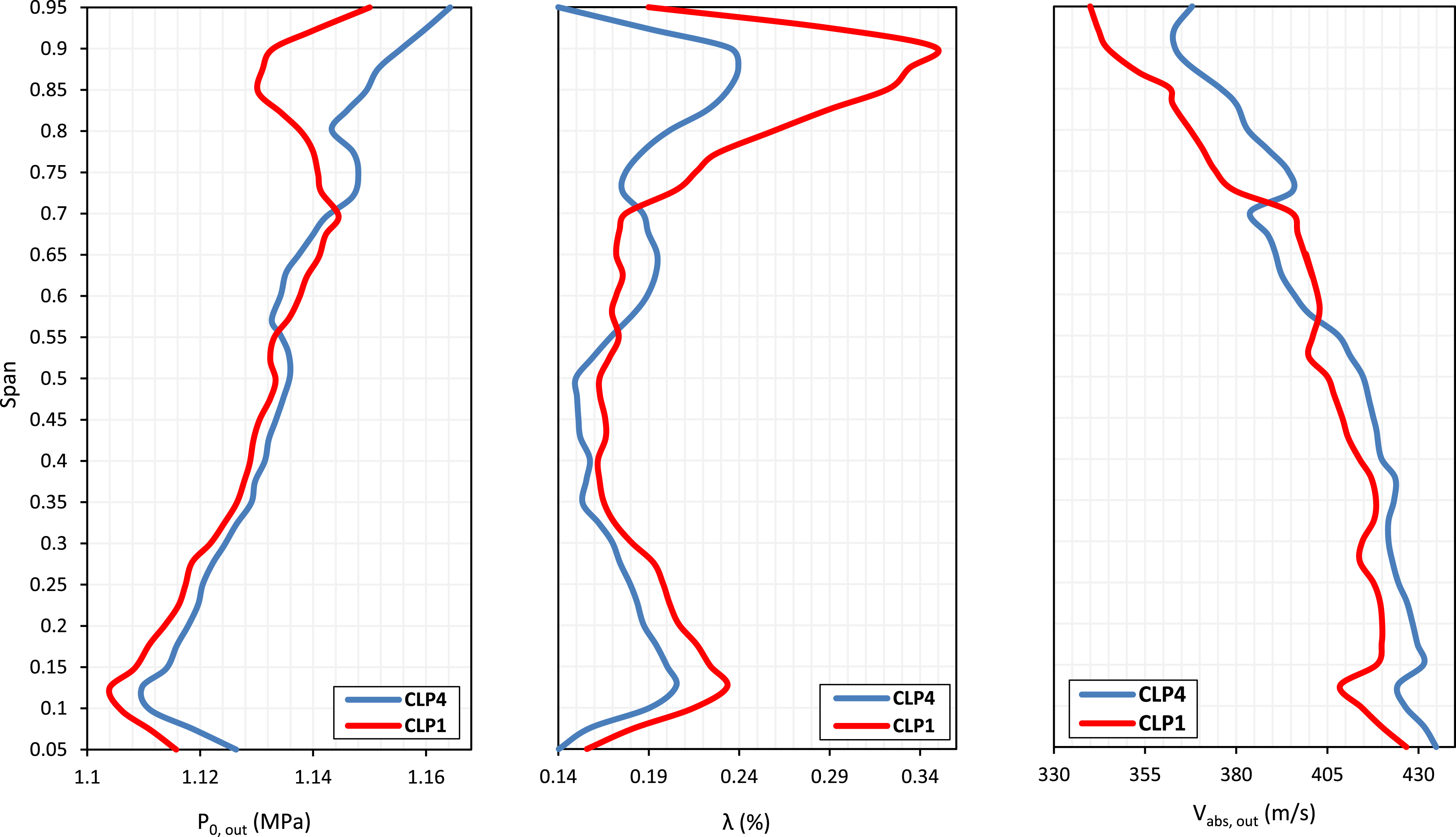
Due to hitting a wake on the S2-2 leading edge in CLP4 case from the hub to mid-span (see Figure 18), outlet total pressure would be higher in comparison to CLP1 case. In contrast, regarding Figure 18, at t/T = 0.5, a wake from hub to around mid-span enters the passage between S2-2 and S2-3 in CLP1, which causes the outlet total pressure to decrease.
Variation of the pressure loss coefficient is directly linked to the total pressure behavior. Also, total pressure is basically influenced by the dynamic pressure (i.e., velocity). Wherever, at a specific span, velocity increases, the total pressure will increase, and vice versa (see Figure 20). It can be detected that in CLP4 case, the outlet velocity and consequently the dynamic pressure are higher in comparison to CLP1, almost along the whole blades span.
Unsteady aerodynamic performance of second rotor
A special form of the pressure coefficient for the rotor blades row can be defined by equation (15), in terms of the exit flow properties.
21

Distribution of instantaneous pressure coefficient on the suction surface (S. S.) and pressure surface (P. S.) of the second rotor blades at mid-span is shown in Figure 21 for CLP1 and CLP4 cases at three normalized times. The area enclosed between these two surfaces indicates the blade loading. The larger area, the higher loading, therefore the more work (i.e., the more lift force) would be produced by the rotor blades. Instantaneous pressure coefficient distributions of second rotor blades at mid-span.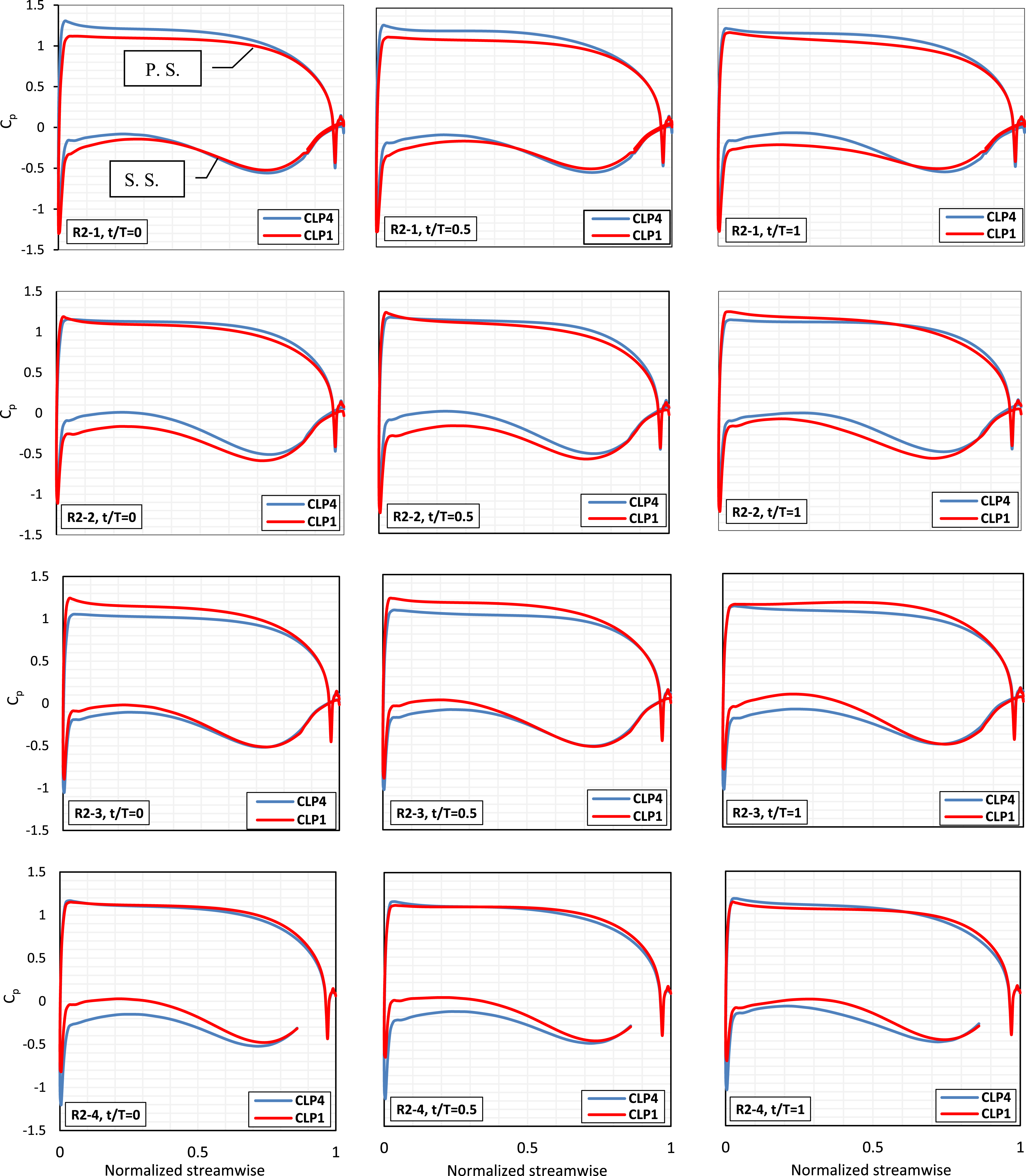
A parameter is introduced to reflect detailed qualitative description of these curves. This parameter, so-called as loading index (LI), represents a dimensionless area enclosed by a curve, similar to the lift coefficient, and is defined by equation (16).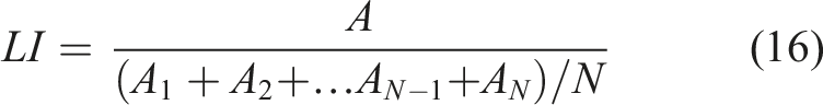
In the above equation, letter A represents the area enclosed by 
Figure 22 shows time-dependent LI variations for the second rotor blades at their mid-span in CLP4 and CLP1 cases. Average values of LI for all the rotor blades are superimposed in these figures, too. In addition, percentage of augmentation of LI in CLP4 in comparison to CLP1 is shown at each time. LI variations for each rotor blade are described as follows. Instantaneous LI of the second rotor blades at mid-span.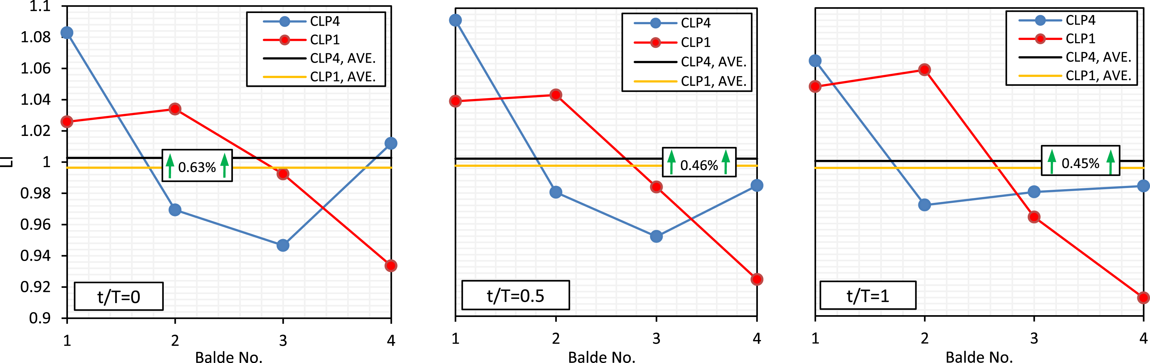
At t/T = 0 in CLP4 case, a wake enters the passage between R2-1 and R2-2 mildly hitting their leading edge and causes velocity to decrease and static pressure to increase on the R2-1 pressure side in comparison to CLP1 case (see Figures 17 and 21). At t/T = 0 in CLP1 case, a wake hits the R2-1 leading edge leaning towards the suction side (see Figure 17, too). With time advancing up to t/T = 1, in CLP1 case, R2-1 loading is increased due to more engaging with the wake. But, in all times in CLP4 in comparison to CLP1, loading (i.e., shown with LI) of R2-1 blade is higher due to higher Cp’s on the pressure side.
At t/T = 0 in CLP1 case, R2-2 is completely covered by a wake flow. Therefore, regarding higher LI, as a result of higher velocity on its suction side, R2-2 has more loading in comparison to CLP4. This superiority continues with time advancing up to t/T = 1. In CLP4 case, a wake flow hits the R2-3 leading edge and sweeps its suction side. A large part of this wake enters the passage between R2-3 and R2-2 and causes static pressure to decrease on R2-3 suction side and to increase on R2-2 pressure side in comparison to CLP1 case (see also Figure 17). In comparison to CLP4 case, growth of R2-2 loading in CLP1 case is higher due to larger Cp’s on its suction side.
Higher Cp on the R2-3 suction side in CLP4 case in comparison to CLP1 case, at t/T = 0, is due to the wake sweeping process on its suction side. But R2-3 pressure side in CLP1 case has higher Cp’s, which causes R2-3 to experience more loading in comparison to CLP4 at t/T = 0 to t/T = 0.5. With time advancing up to t/T = 1, R2-3 in CLP4 case shows higher loading, since the fluid particles velocities are increased on its suction side (see Figure 21).
In CLP4 case, a strong wake impinges on the R2-4 leading edge and sweeps its pressure and suction sides (see Figure 17). In CLP1 case, a wake enters the passage between R2-4 and corresponding blade R2-1. Hence, the better blade-wake interaction in CLP4 case causes more Cp’s on the suction and pressure sides which results in higher loading for R2-4 at all times (see Figures 21 and 22) in comparison to CLP1 case. With time advancing in CLP4 case, R2-4 gets rid of the wake flow and consequently its loading decreases.
Conclusion
Zonal DES turbulence modeling and rotor-stator transient approach are implemented for three-dimensional unsteady flow simulations within the first two stages of a 4-stage low pressure turbine at six different clocking configurations of the second stator blades. Investigation on aerodynamic performance and blade-wake interaction are the main target of the present research work. Phenomenology of the wake deformation and its transient properties within the blades passages is studied, precisely. The main conclusions drawn from the current research work are as follows: ✓ Results of three-dimensional simulations, based on DES turbulence modeling, reveal lower fluctuations in flow properties at the vicinity of blade surfaces in comparison to URANS, promising priority of the former method to the latter one. ✓ Wake deformation composed of bowing, re-orientation, stretching, and elongation are identified, precisely. Based on lift and pressure coefficient results, it was possible to introduce three time intervals assigned by “wake weakness,” “wake domination,” and “wake dissipation.” ✓ The fourth clocking position (CLP4) is identified as the optimum clocking case, in which, inlet total pressure and output power of second rotor are increased by 0.099% and 0.336%, respectively, in comparison to the worst case (CLP1). So the total-to-total efficiency of the second rotor blades row is increased by 0.35%. ✓ Total output power of the whole two stages in the optimum case (CLP4) is increased by 0.237% in comparison to the worst case (CLP1). ✓ In the optimum clocking case, total pressure loss is reduced due to impinging the wake flow on the second stator blade leading edge, which results in higher total pressure at the second rotor inlet. ✓ Unsteady analyses of the blade-wake interaction in the second rotor indicate that loading can be increased while the wake flow covers the whole rotor blade surface or impinges its leading edge. This is a situation which exclusively occurs in the optimum clocking position, and results in accelerating flow on the blade suction side or decelerating flow on the pressure side.
Footnotes
Acknowledgments
The authors would like to thank the Gas Turbine Institute of the Iran University of Science and Technology for supporting this research work.
Declaration of conflicting interests
The author(s) declared no potential conflicts of interest with respect to the research, authorship, and/or publication of this article.
Funding
The author(s) received no financial support for the research, authorship, and/or publication of this article.