A modified dual time integration technique for aerodynamic quasi-static and dynamic stall hysteresis

Abstract

Simulation of the aerodynamic stall phenomenon in both quasi-static and dynamic conditions requires expensive computational resources. The computations become even more costly for static stall hysteresis using an unsteady solver with very slow variation of angle of attack at low reduced frequencies. In an explicit time-marching solver that satisfies the low Courant number condition, that is, $CFL\le 1$ , the computational cost for such simulations becomes prohibitive, especially at higher Reynolds numbers due to the presence of thin-stretched cells with large aspect ratio in the boundary layer. In this paper, a segregated solver method such as the Semi-Implicit Method for Pressure-Linked Equations (SIMPLE) is modified as a dual pseudo-time marching method so that the unsteady problem at each time step is reformulated as a steady state problem. The resulting system of equations in the discretized finite volume formulation is then reduced to zero or near-zero residuals using available convergence acceleration methods such as local time stepping, multi-grid acceleration and residual smoothing. The performance and accuracy of the implemented algorithm was tested for three different airfoils at low to moderate Reynolds numbers in both incompressible and compressible flow conditions covering both attached and separated flow regimes. The results obtained are in close agreement with the published experimental and computational results for both quasi-static and dynamic stall and have demonstrated significant savings in computational time.

Introduction

Hysteresis phenomena in aerodynamics at high angles of attack still attract high interest both in experimental and computational studies.^1–6 Hysteresis loops can occur even at very low reduced frequencies, that is, $k=\frac{\omega c}{2U_{ref}}\le 0.002$ , with a continuous periodical change in angle of attack or in static conditions indicating a bi-stability of two different separated flow patterns at the same angle of attack. Computer simulations of static stall hysteresis are reported less commonly in the literature than simulations of dynamic stall hysteresis. This can be due to a high sensitivity to the choice of turbulence model, fineness and adaption of the grid, the time integration technique used to advance the simulation, etc.

It is widely believed among some researchers that static hysteresis is related to the formation and breakdown of a laminar separation bubble (LSB) on the suction side of the airfoil under low to moderate Reynolds number flow conditions.^2,7 The authors in Ref. 7 used four different transitional turbulence models to predict the hysteresis in the flow past the NACA 0018 airfoil at $Re=0.3\times {10}^6.$ Based on their obtained computational results, it was concluded that the transitional models work well for predicting LSB at low angles of attack but fail to predict the magnitude and effects associated with static hysteresis. Using other turbulence models, such as the Baldwin–Lomax,^3,4 Spalart–Allmaras (SA) and the Shear Stress Transport (SST)^5,6 models, it may be possible to capture static hysteresis loops, but they cannot predict the LSB. Thus, it can be stated that, due to the sensitivity of hysteresis to the choice of turbulence modelling, the use of RANS simulations to predict the phenomenon of quasi-static hysteresis requires significant further research.

On the contrary, dynamic stall hysteresis is more robust and has been reported extensively in the literature in both computational and experimental studies. Dynamic stall is often associated with transient flow structures during the upstroke phase with generation of leading edge vortices (LEVs) propagating downstream along with separation from the trailing edge and reattachment of flow during the downstroke phase on return to low angles of attack.^8–14 It should be noted that the presence of transitional flow even at moderately high Reynolds numbers is associated with the leading edge LSB which influences the peak suction pressure, ¹¹ and hence, transitional models might improve the predictions during the upstroke. ¹⁵ On the other hand, there are uncertainties and discrepancies in the downstroke motion due to deficiencies in transition models ¹¹ for fully separated flow conditions.

The main purpose of this paper is to implement a modified dual time integration method to reduce simulation time required in prediction of quasi-static and dynamic hysteresis phenomena. This goal was reached through the development of a computational algorithm by introducing a pseudo-time derivative to the segregated solver methods such as the Semi-Implicit Method for Pressure-Linked Equations (SIMPLE) algorithm. ¹⁶ SIMPLE algorithm is well known for its steady state convergence and stability.^16,17 The unsteady problem, due to continuous change of angle of attack in both quasi-static and dynamic stall motions, can be reformulated as a steady-state problem to be marched in an artificial time for a given physical time step. This modification can be characterized as a variant of the dual time stepping (DTS) technique and is implemented and tested in OpenFOAM, an open source CFD code. ¹⁸ OpenFOAM has been successfully applied for prediction of external aerodynamics with separated flow condition.^6,19,20 In Ref. 19, OpenFOAM was validated for prediction of aerodynamic autorotation against results obtained at the Netherlands Aerospace Centre (NLR) using the in-house CFD code ENFLOW. ²¹ OpenFOAM also demonstrated comparable accuracy against commercial CFD codes Star-CCM+ and Fluent at the AIAA High Lift Prediction Workshop. ²⁰

The DTS scheme was first introduced by Jameson in Ref. 22 by inclusion of a pseudo-time often denoted by $t^{*}$ or $\tau$ along with physical time t. For the discretization of physical time, a second order accurate Euler backward method was used. ²² The DTS technique is almost always employed with a compressible solver.^23–26 The use of DTS technique with incompressible flow solvers has also been carried out to some extent and is accomplished by introducing artificial compressibility. ²⁷ The compressible flow solvers which employ DTS often resort to introducing artificial dissipation and preconditioning, especially at low Mach numbers. The method proposed in this paper can be successfully employed in both the incompressible and compressible flow regime/solvers.

The computational robustness and sensitivity of the implemented incompressible and compressible DTS technique are tested by simulating the quasi-static and dynamic stall hysteresis phenomena in flow past the NACA 0012, 0015 and 0018 airfoils at a moderate range of Reynolds number $1.35\times {10}^5\le Re\le 2\times {10}^6$ and Mach number $0.0135\le M\le 0.2$ using OpenFOAM.^18,28,29 The unsteady Reynolds-averaged Navier–Stokes (URANS) equations are solved in conjunction with the SA ³⁰ and the SST ³¹ turbulence models for closure. The hysteresis phenomena simulated for all airfoils are in good agreement with the available experimental data and published CFD simulation results confirming the reliability of the implemented dual time algorithm. The sensitivity of the simulation results to the parameters of the computational framework is discussed along with considerations of the physical aspects of the quasi-static and dynamic hysteresis processes.

The paper is organized as follows. The section ‘Modified Dual Time Algorithm Implemented in OpenFOAM’ outlines the implemented solver method. The section ‘Computational Framework’ presents details of the computational domain, grid independence study and details of the numerical setup for the considered case studies. The results obtained for oscillatory pitching motion for the NACA 0015 and NACA 0012 airfoils are presented in the section ‘Computational Results’ together with a simulation of the static hysteresis phenomenon experimentally observed on the NACA 0018 airfoil. The concluding remarks are presented in the last section.

Modified dual time algorithm implemented in OpenFOAM

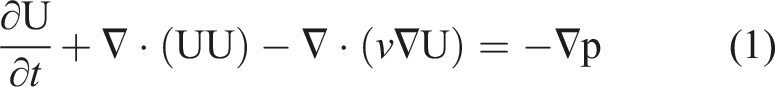
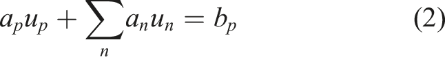
The momentum equation for incompressible flow is: ³²

$\frac{\partial \mathrm{U}}{\partial t}+\nabla ·\left(\mathrm{U}\mathrm{U}\right)-\nabla ·\left(\nu \nabla \mathrm{U}\right)=-\nabla \mathrm{p}$

(1)

Applying the finite volume method (FVM), equation (1) can be written in the following semi-discretized form:^17,32

$a_p{u}_p+\sum _n{a}_n{u}_n=b_p$

(2)

where $a_p$ and $a_n$ are the matrix coefficients associated with centre point $p$ and neighbour point $n$ and b _p represents the source term. In matrix notation, equation (2) can also be expressed as:^17,28

$GX=R$

(3)

where $G$ is the matrix holding the finalized coefficients of FVM discretizations for centre point $p$ and neighbouring element n around the computational stencil, $X$ is the solution vector and $R$ is the right-hand side (RHS). Matrix $G$ is decomposed for the diagonal and off-diagonal elements as:

$G=A+H^{\prime }$

(4)

where matrix $A$ is composed from the diagonal elements of matrix $G$ and matrix $H^{\prime }$ includes the off-diagonal elements of matrix $G$ .

Replacing $G$ in equation (3) with expression in equation (4) gives

$\left(A+H^{\prime }\right)X=R$

(5)

The right-hand side of equation (5) can be grouped together as:

$AX=R-H^{\prime }X$

(6)

Denoting $H=R-H^{\prime }X$ , one can rewrite equation (6) as shown below:

$AX=H$

(7)

Matrix A in equation (7) includes the diagonal coefficients of the discretized FVM matrix for flow variables at grid locations, $X$ is the solution vector and $H$ is the RHS, which contains the source terms (excluding pressure gradient) and the off-diagonal elements of matrix G multiplied by their velocities. ³²

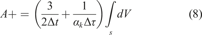
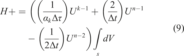
The DTS contribution to the system of discretized matrix coefficients in equation (7) can now be denoted as:

$A+=\left(\frac{3}{2\mathrm{\Delta }t}+\frac{1}{{\alpha }_k\mathrm{\Delta }\tau }\right)\underset{s}{{\displaystyle \int }}dV$

(8)

$H+=\left(\left(\frac{1}{{\alpha }_k\mathrm{\Delta }\tau }\right)U^{k-1}+\left(\frac{2}{\mathrm{\Delta }t}\right)U^{n-1}-\left(\frac{1}{2\mathrm{\Delta }t}\right)U^{n-2}\right)\underset{s}{{\displaystyle \int }}dV$

(9)

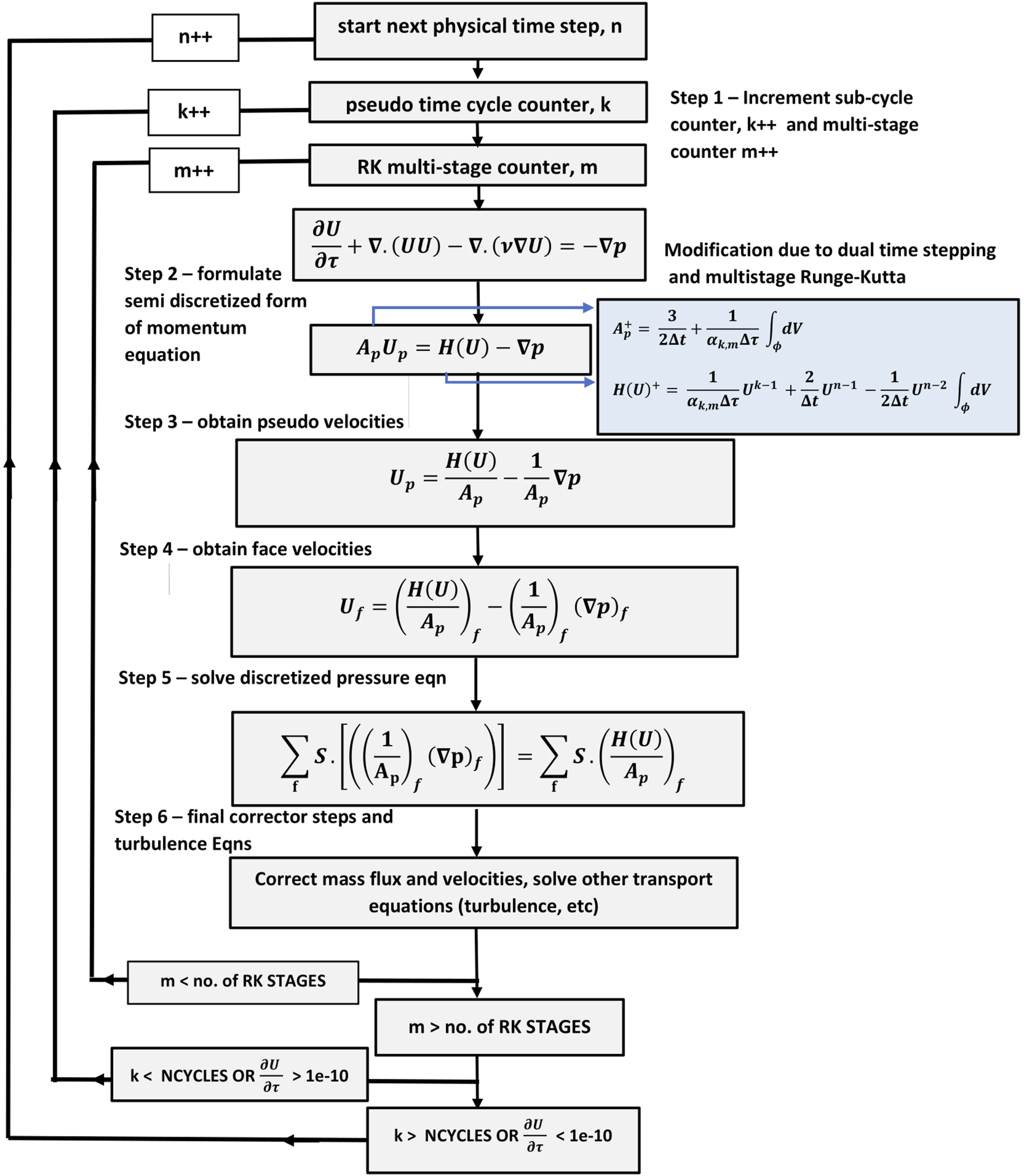
where n in equation (9) is the physical time step number, $k$ is the sub-cycle iteration number within each time step corresponding to pseudo-time, ${\alpha }_k$ is the Runge–Kutta coefficient in each stage and $\underset{s}{{\displaystyle \int }}dV$ is the integrated volume of each element. $A+$ in equation (8) denotes the dual time contribution to the diagonal elements of $A_p$ , and $H+$ in equation (9) denotes the additional source term contribution to the $H\left(U\right)$ term due to the two previous physical time steps $n-1$ and $n-2$ (see Figure 1). The use of the modified DTS method with segregated solver methods gives a reasonable advantage as the 3/2 $∆t$ diagonal term can be treated in an implicit manner along with a multi-stage Runge–Kutta scheme ²⁴ where multi-grid methods can be further used to accelerate convergence.

Figure 1.

Modified dual time stepping algorithm for incompressible flows.

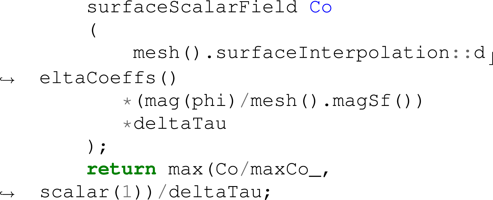
Listing 1: Local time stepping in OpenFOAM.

The term $∆\tau$ is obtained by a slight modification of a local time stepping method known as the ‘CoEuler’ method which is already implemented in OpenFOAM. ²⁸ The modification brought is to allow the maximum allowable local time step to be determined by the pseudo-time step size and by the specified maximum local Courant number rather than the physical time step size and the global Courant number. This implementation ensures a stabilized pseudo-time step size so that the diagonal dominance is maintained in the FVM matrix. ³² The local time stepping method used in OpenFOAM is shown in Listing 1.

The deltaCoeffs in Listing 1 are the reciprocal of cell centre to centre distances projected over the normal face areas, phi refers to the mass flux at cell face, magSf is the magnitude of the normal vectors and deltaTau is the pseudo-time step size. The implemented algorithm as a flow chart is shown in Figure 1.

A similar concept as shown in Figure 1 is used in the implementation of a modified compressible DTS method based on segregated solver algorithms. The main difference to the incompressible dual time algorithm is the modification of the density and the energy equation further to the momentum equations, all of which now need to be marched in a pseudo-time. The variants of the segregated solver methods such as SIMPLE, SIMPLEC, SIMPLER and PIMPLE algorithms are understudied in this research, as this was not the primary motivation, but remains as a future work.

Computational framework

This section summarizes the adopted computational framework for analysis of quasi-static and dynamic stall conditions in OpenFOAM.

Geometry and grid generation

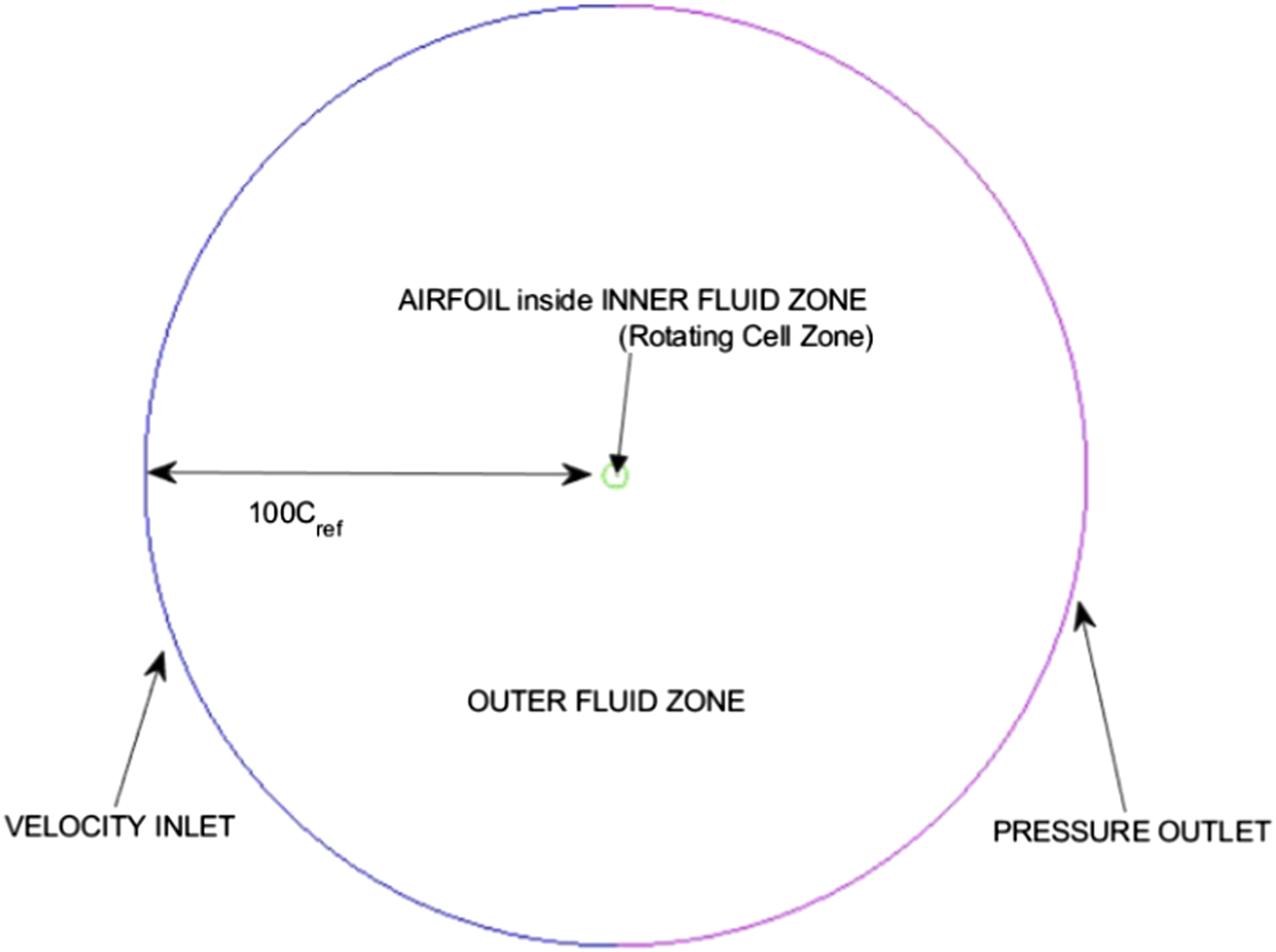
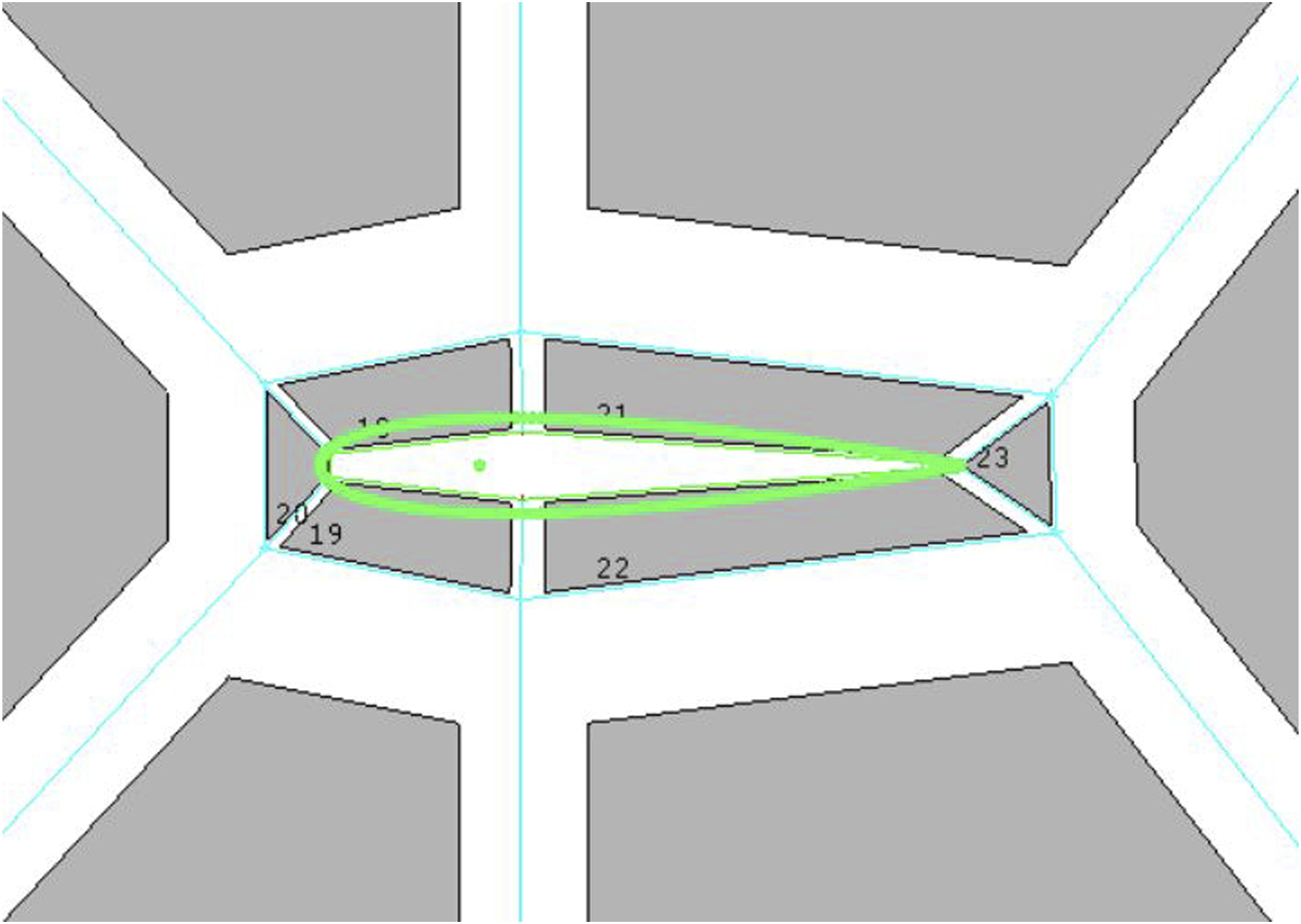
The computational domain is created by placing the airfoil at least 100 chord lengths away from the inlet and outlet. The domain considered for the case studies is shown in Figure 2. Computational grids for the NACA 0012 and NACA 0015 airfoils are generated using a two-zone approach with an inner fluid zone set to be the rotating zone around quarter-chord of the airfoil which also coincides with the centre of the circular shaped inner fluid zone. The outer fluid zone is at static conditions and does not rotate. Both zones are merged using an Arbitrary Mesh Interface (AMI) with nearly equal number of elements and almost similar cell spacing. For this AMI approach, a range of 80–100% cell size match is encouraged to enable a smooth flow field interpolation between the AMI interfaces. In the multi-zone approach, the considered blocking strategy is an O-type, as shown in Figure 3. This type of blocking is beneficial, as the blocking shape naturally converges from far field towards a blunt-trailing edge airfoil shape and minimizes any non-orthogonality or cell skewness issues that might develop in other types of blocking.

Figure 2.

The computational domain used for quasi-static and dynamic stall analysis.

Figure 3.

Adopted blocking strategy for the inner fluid zone.

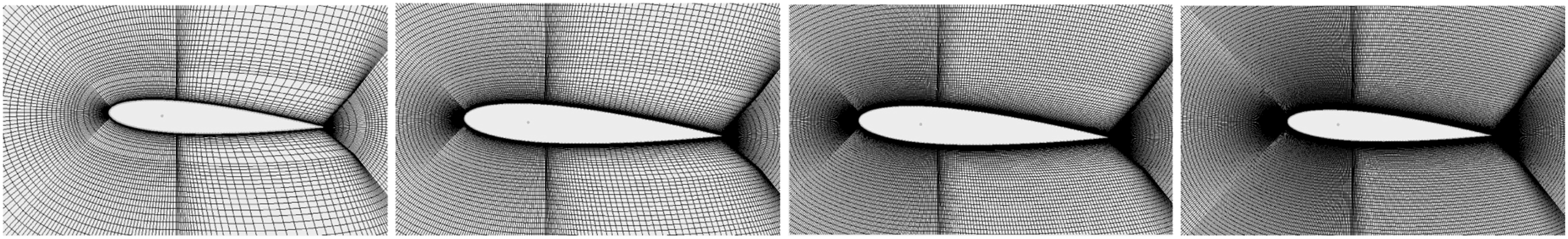
The boundary layer is resolved using the low wall Y + criterion with $Y+\le 1$ , that is, unity, with more than 40 adjacent boundary layers and a cell growth ratio of 1.1 along the normal direction. The resulting grids ranged from 100,000 to 250,000 quadrilateral elements. A mesh independent solution was obtained between the medium and the extra-fine grid with 100,000−200,000, which exceeds the grid requirements specified in Refs. 11 and 15 for evaluation of dynamic stall in flow past the NACA 0015 airfoil. The generated multi-zone grid for the NACA 0015 airfoil is shown in Figure 4. The considered refinement from coarse to extra-fine grid is shown in Figure 5.

Figure 4.

Multi-zone grid generated for the NACA 0015 airfoil at $Re=2\times {10}^6$ .

Figure 5.

Refinement considered (coarse, medium, fine and extra-fine) for the multi-zone grid adopted for the NACA 0015 airfoil at $Re=2\times {10}^6$ .

The computational grid for the NACA 0018 airfoil is a single-zone grid, and when in motion, the entire grid rotates around the centre of moment of the airfoil. The reason for having a different approach of grid generation for the NACA 0018 airfoil is to keep mesh consistency with our previous work of static hysteresis approach in Ref. 5. The grid size for the NACA 0018 airfoil is 110,000 quad elements, and the boundary layer is resolved in the low wall Y+ region using $Y+\le 1$ . In addition, the sensitivity of the data interpolation between mesh interfaces in an AMI approach due to rotating zones was avoided by using a single grid. This was done to ensure maximum robustness for the NACA 0018 case as quasi-static stall hysteresis is more sensitive to flow and mesh parameters than dynamic stall cases.

Numerical setup for the case studies

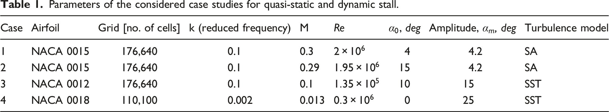
Flow conditions and airfoil motion parameters used for the employed case studies are shown in Table 1. The mesh motion in all case studies follows harmonic variations of the angle of attack α in the form $\alpha \left(t\right)={\alpha }_0+{\alpha }_m\mathit{sin}\left(\omega t\right)$ .The free-stream boundary conditions are the generally considered velocity inlet with fixed value specific at the boundary, pressure outlet with zero gradient condition. The boundary condition for the pitching airfoil is the ‘movingWallVelocity’ function, which ensures a zero flux condition through a moving boundary. The time step in all considered cases was determined by considering a physical time step size of interest, whilst not exceeding $0.1c/U_{ref}$ which is 1/10^th of the convective time.

Table 1.

Parameters of the considered case studies for quasi-static and dynamic stall.

Case	Airfoil	Grid [no. of cells]	k (reduced frequency)	M	Re	${\alpha }_0$ , deg	Amplitude, ${\alpha }_m$ , deg	Turbulence model
1	NACA 0015	176,640	0.1	0.3	$2\times {10}^6$	4	4.2	SA
2	NACA 0015	176,640	0.1	0.29	$1.95\times {10}^6$	15	4.2	SA
3	NACA 0012	176,640	0.1	0.1	$1.35\times {10}^5$	10	15	SST
4	NACA 0018	110,100	0.002	0.013	$0.3\times {10}^6$	0	25	SST

Two case studies (Cases 1 and 2) for the NACA 0015 airfoil are carried out approximately at the same Reynolds number of $Re=2.0\times {10}^6$ and Mach number $M=0.1$ with a reduced frequency of k = 0.1. In the first case, an angle of attack range of $\alpha \left(t\right)={4.0}^{\circ }\pm \hspace{0.17em}{4.2}^{\circ }\mathit{sin}\left(\omega t\right)$ $\left(\omega =2\pi f\right)$ is characterized by the attached flow conditions. In the second case, the variation of angle of attack of $\alpha \left(t\right)={15.0}^{\circ }\pm \hspace{0.17em}{4.2}^{\circ }\hspace{0.17em}\mathit{sin}\left(\omega t\right)$ lies in the separated flow region. In case studies 1 and 2, experiments presented in Ref. 8 were tripped at the leading edge, and therefore, fully turbulent flow conditions were expected as mentioned in Ref. 15, and hence, transitional turbulence models were not used. The SA turbulence model ³⁰ was used for both cases. The SA model solves a single partial differential equation for the modified turbulent viscosity $\widehat{\nu }$ . Both the compressible and the incompressible dual time solvers implemented in OpenFOAM are used in these cases as the dynamic stall with high reduced frequency of $k=0.1$ can lead to a localized transonic flow regime, especially in the near vicinity of the leading edge. ¹¹

The NACA 0012 airfoil simulation (Case 3) was carried out at a much lower Reynolds number of $Re=\mathrm{135,000}$ , reduced frequency $k=0.1$ and a large oscillation amplitude of ${15.0}^{\circ }.$ While the flow Reynolds number for this case is in laminar–turbulent transition zone at $Re=\mathrm{135,000}$ , the experimental researchers in Ref. 33 concluded that the leading edge (LE) dynamic stall did not occur with the bursting of a laminar separation bubble, but with a sudden turbulent breakdown at a short distance downstream of the leading edge. ³³ And therefore, a transitional turbulence model was not employed for this case but the two equation SST turbulence model ³¹ was used. The SST model solves two equations, that is, the turbulent kinetic energy and the specific dissipation rate of turbulence. For this case, the incompressible dual time solver is used as the free-stream Mach number is much lower at $M=0.1$ .

The last case study, that is, Case 4 for the NACA 0018 airfoil was carried out using the incompressible dual time solver at Reynolds number of $Re=0.3\times {10}^6$ with the intention of capturing the quasi-static aerodynamic stall hysteresis using a significantly reduced frequency of $k=0.002$ . The experimental results for this case were taken from Ref. 2, and it was not clear whether the LE of the airfoil was tripped in the experiment. Furthermore, as we are more focused in the fully separated flow conditions with the ‘Bottom-Branch’ of quasi-static hysteresis and for keeping consistency in comparison with the simulated aerodynamic hysteresis loop published in Ref. 5, the SST turbulence model was used.

Grid independence and further validation

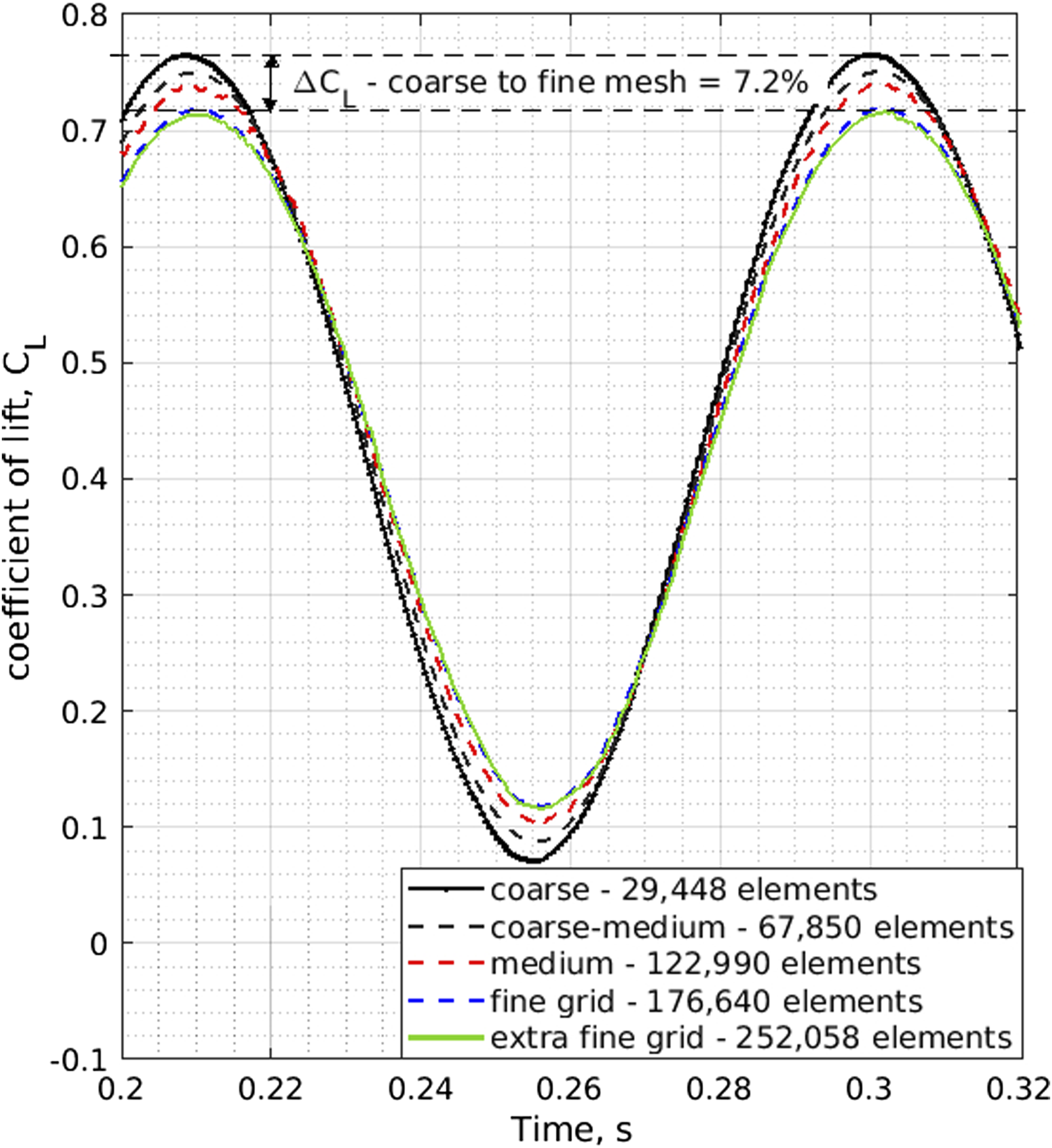
The grid independence is studied by conducting pitch cycle simulations of the NACA 0015 airfoil with a non-dimensional reduced frequency of $k=0.1$ using five different levels of grids ranging from coarse to extra-fine mesh resolution. Case 1 is taken as a base case for grid independence studies for the NACA 0015 and NACA 0012 airfoils, and if the dynamic variation of the lift coefficient C_L for one cycle of pitch oscillation remains similar, the obtained solution can be said to be independent from the resolution of the grid. The reason for using such an approach is to qualitatively determine a grid refinement level which will produce mesh independent results not just for static simulations but also for a dynamically deforming grid where mesh flux is an important criterion to be considered.

The obtained results shown in Figure 6 demonstrate that the maximum difference between the coarse to fine mesh is at 7.2%. There is almost negligible deviation in the peak lift coefficient between the fine grid (blue dashed line) and the extra-fine grid (green solid line), and hence, the fine grid with 176,640 elements will be used for the rest of the simulations for both NACA 0015 and NACA 0012 airfoil case studies.

Figure 6.

Mesh independence results obtained for Case 1 using NACA 0015 airfoil at $Re=2\times {10}^6$ .

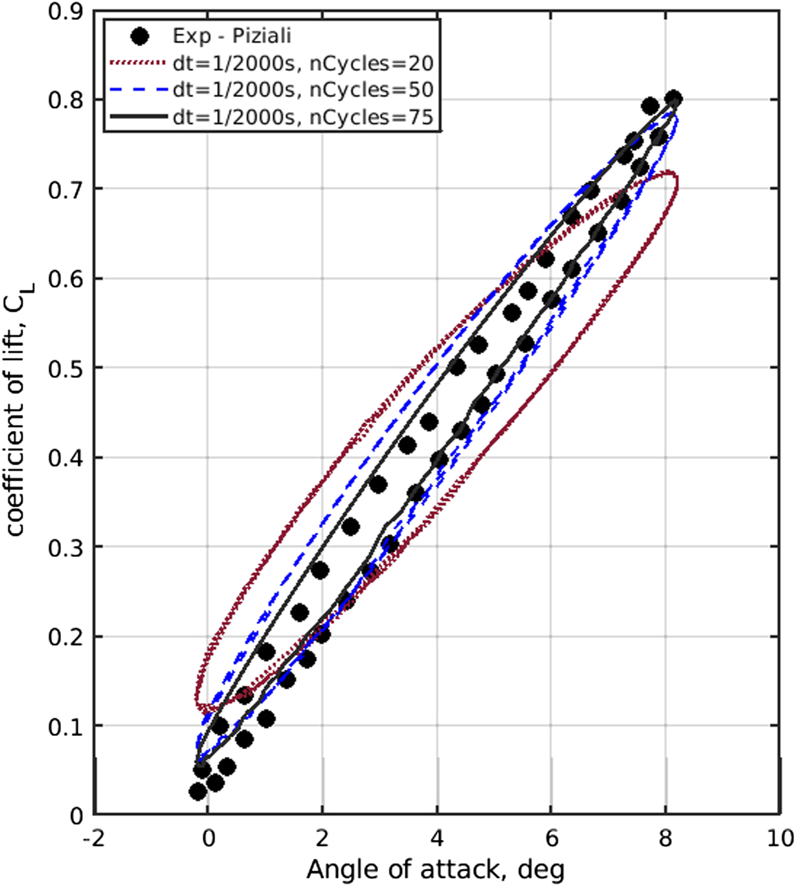
Once a grid independent solution was obtained, a pseudo-time step convergence study was conducted to investigate the required number of sub-cycles in pseudo-time. The obtained results for this study shown in Figure 7 demonstrate that 50−75 sub-cycles in pseudo-time marching are adequate and adding any further sub-cycles does not improve the results significantly. Furthermore, the obtained results are verified against Piziali’s experimental results from Ref. 8, and it is evident that the lift coefficient obtained during the pitch cycle is certainly not an outlier.

Figure 7.

Pseudo sub-cycle convergence study for Case 1 at $Re=2\times {10}^6$ .

Computational results

This section presents the computational results obtained for the dynamic stall cases carried out with NACA 0012 and NACA 0015 airfoils along with quasi-static stall hysteresis case for the NACA 0018 airfoil. A summary of the considered case parameters can be referred to in Table 1. The two case studies considered for the NACA 0015 airfoil with aerodynamic chord $c=0.294m$ are conducted approximately at the same Reynolds number of $Re\approx 2\times {10}^6$ and a reduced frequency of $k=0.1$ . In the first case, the NACA 0015 airfoil oscillates in the angle of attack range where the flow remains attached. In the second case, the NACA 0015 airfoil oscillates in the angle of attack range covering the stall zone, and during the upstroke motion, there is a significant development of flow separation and during the downstroke phase a delayed reattachment of flow occurs.

Case 1: Attached flow past NACA 0015 airfoil at $Re=2\times {10}^6$

During an oscillatory cycle in the angle of attack with an amplitude of ${\alpha }_m={4.2}^{\circ }$ and a mean angle of ${\alpha }_0={4.0}^{\circ }$ , the flow remains attached to the airfoil, forming a small trailing wake behind the airfoil with periodic changes in the vorticity sign. ³⁴ The wake of distributed vortices induces time-dependent variations in the airfoil local angle of attack resulting in changes in the so called in-phase and out-of-phase aerodynamic derivatives.

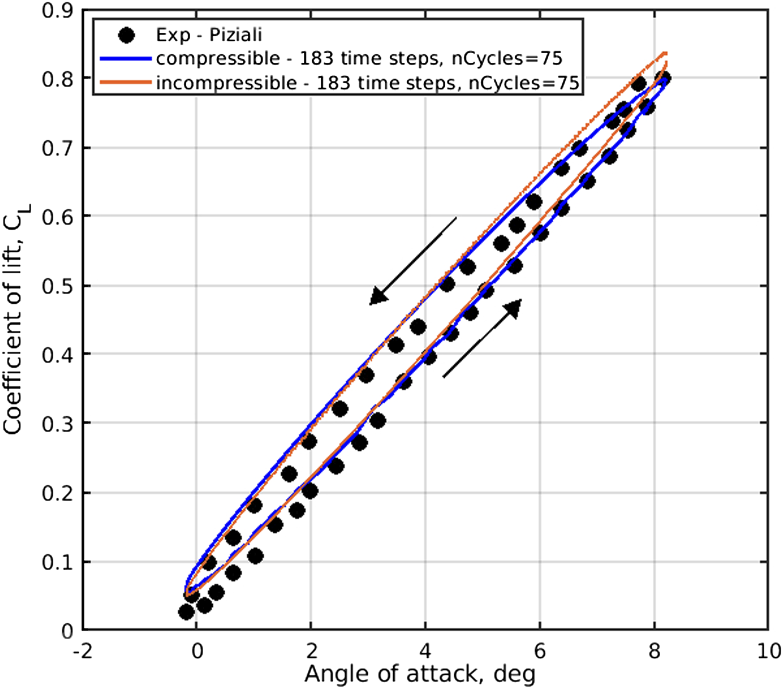
These changes are reflected in the slope of the average lift force coefficient dependence on angle of attack and in the thickness of the elliptical dynamic loop representing the normal force coefficient during the oscillation cycle. The simulation was conducted with 183 time steps per pitch cycle corresponding to a physical time step size of $\mathrm{\Delta }t=0.0005s$ and 75 sub-cycles per time step.

The simulation results are shown in Figure 8 for the lift force coefficient C _L . It can be seen that the OpenFOAM compressible simulation results during the oscillatory pitch cycle are in excellent agreement with the experimental results from Piziali’s experimental data. ⁸ For low angles of attack $\alpha \le {5.0}^{\circ }$ , both the incompressible and compressible solvers implemented in this study produce very similar results. At an angle of attack exceeding $\alpha \ge 5$ degrees, the compressible solver results are in much closer agreement with the experimental data. This is due to the better prediction of the density changes in close vicinity of the leading edge, associated with the localized transonic flow regime in this region due to the high reduced frequency of $k=0.1$ .

Figure 8.

Lift force coefficient $C_L$ for the NACA 0015 airfoil in periodical motion $\alpha \left(t\right)=4^{\circ }+{4.2}^{\circ }\hspace{0.17em}\mathit{sin}\left(\omega t\right)$ with $k=0.1$ , $Re=2\times {10}^6$ and $M=0.3$ .

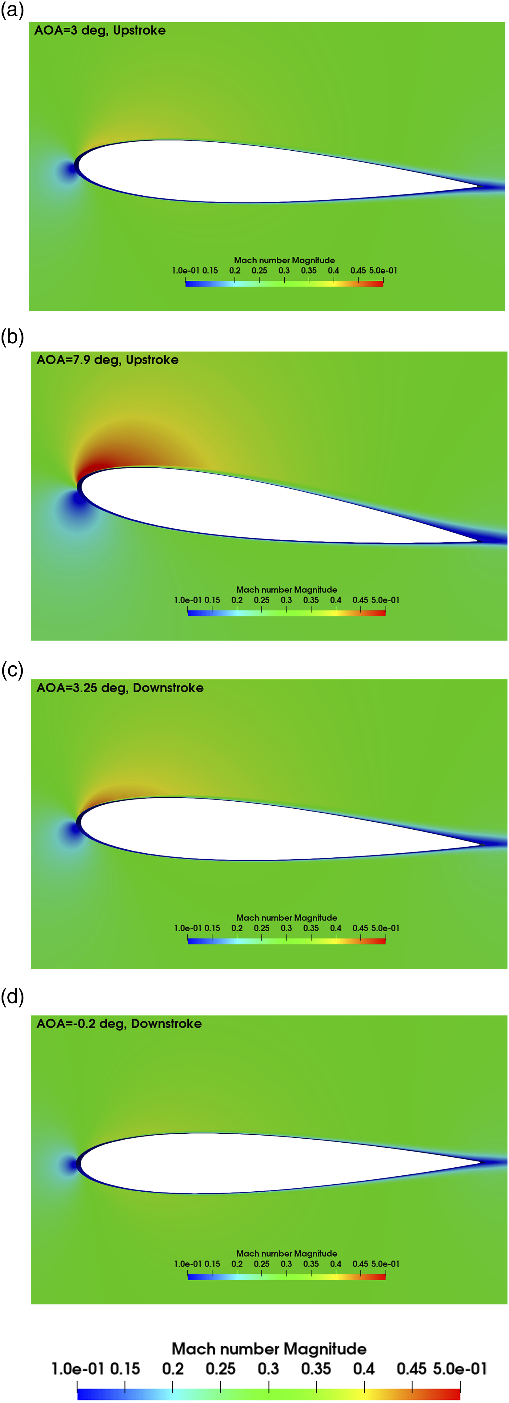
The slope and thickness of the $C_L$ elliptical cycle depend on the reduced frequency parameter k as elaborated in Ref. 34. For this case, the hysteresis is anti-clockwise as shown by the arrows in Figure 8. The reason for this anti-clockwise loop in the lift coefficient is due to the increased velocity on the suction side near the LE of the airfoil during the downstroke motion. This can be visually observed by comparing the contours of Mach number magnitude at $\alpha \approx 3^{\circ }$ during the upstroke motion and downstroke motion in Figure 9. The intensity of red zone, showing the Mach number $M\ge 0.5$ , near the leading of the suction side of the airfoil is much higher in Figure 9(c) corresponding to the ${3.0}^{\circ }$ during downstroke motion, when compared with the upstroke motion shown in Figure 9(a).

Figure 9.

Contours of Mach number during pitch cycle with $\alpha \left(t\right)=4^{\circ }+{4.2}^{\circ }\hspace{0.17em}\mathit{sin}\left(\omega t\right)$ , $k=0.1$ , $Re=2\times {10}^6$ and $M=0.3$ : (a) upstroke – $\alpha \left(t\right)={3.0}^{\circ }$ , (b) upstroke – $\alpha \left(t\right)={7.9}^{\circ }$ , (c) downstroke – $\alpha \left(t\right)={3.25}^{\circ }$ and (d) downstroke – $\alpha \left(t\right)=-{0.2}^{\circ }$ .

It is also evident that the flow is mostly attached with only mild trailing edge separation during the pitch cycle simulation for the NACA 0015 airfoil in motion with $\alpha \left(t\right)=4^{\circ }+{4.2}^{\circ }\hspace{0.17em}\mathit{sin}\left(\omega t\right)$ and $k=0.1$ . When the angle of attack increases the trailing edge separation point towards the LE and in the upstroke motion at $\alpha \left(t\right)={7.9}^{\circ }$ , the separation point is approximately at about 60% of the chord.

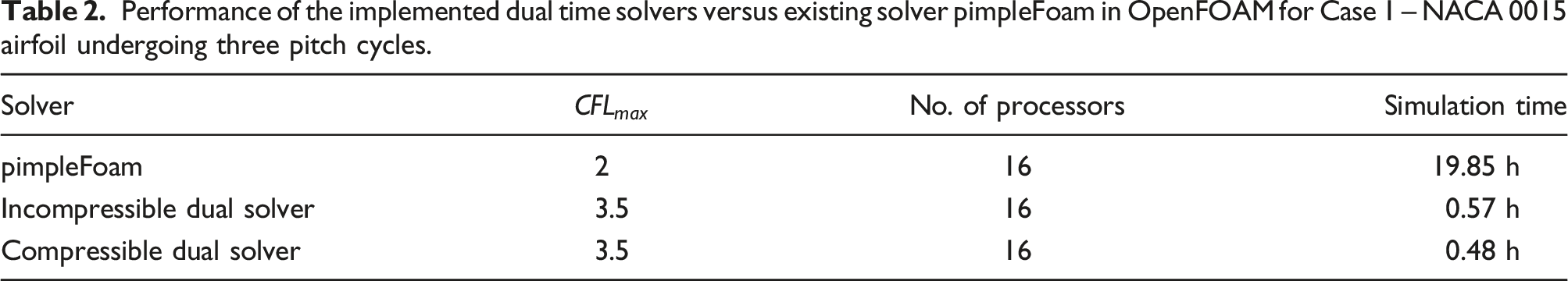
The performance of the dual time solvers implemented in this study compared with OpenFOAM’s unsteady solver pimpleFoam (incompressible) is shown in Table 2. Both the incompressible and compressible dual time solvers show a significant amount of computational time savings due to being able to use a larger global time step but still keep the desired accuracy by maintaining the maximum local CFL below $CFLmax\le 3.5$ .

Table 2.

Performance of the implemented dual time solvers versus existing solver pimpleFoam in OpenFOAM for Case 1 – NACA 0015 airfoil undergoing three pitch cycles.

Solver	$CF{L}_{\mathit{max}}$	No. of processors	Simulation time
pimpleFoam	2	16	19.85 h
Incompressible dual solver	3.5	16	0.57 h
Compressible dual solver	3.5	16	0.48 h

Case 2: Deep stall – NACA 0015 airfoil at $Re=2\times {10}^6$

In this case, the range of the angle of attack is shifted upwards to cover the pre/post stall zone with large massive flow separation. The airfoil angle of attack during the pitch cycle is characterized by $\alpha \left(t\right)={15}^{\circ }+{4.2}^{\circ }\hspace{0.17em}\mathit{sin}\left(\omega t\right)$ , where reduced frequency $k=0.1$ . This angle of attack variation allows to validate OpenFOAM simulations with the implemented DTS method in predicting dynamic hysteresis phenomenon against results from Ref. 11 and experimental results from Piziali in Ref. 8.

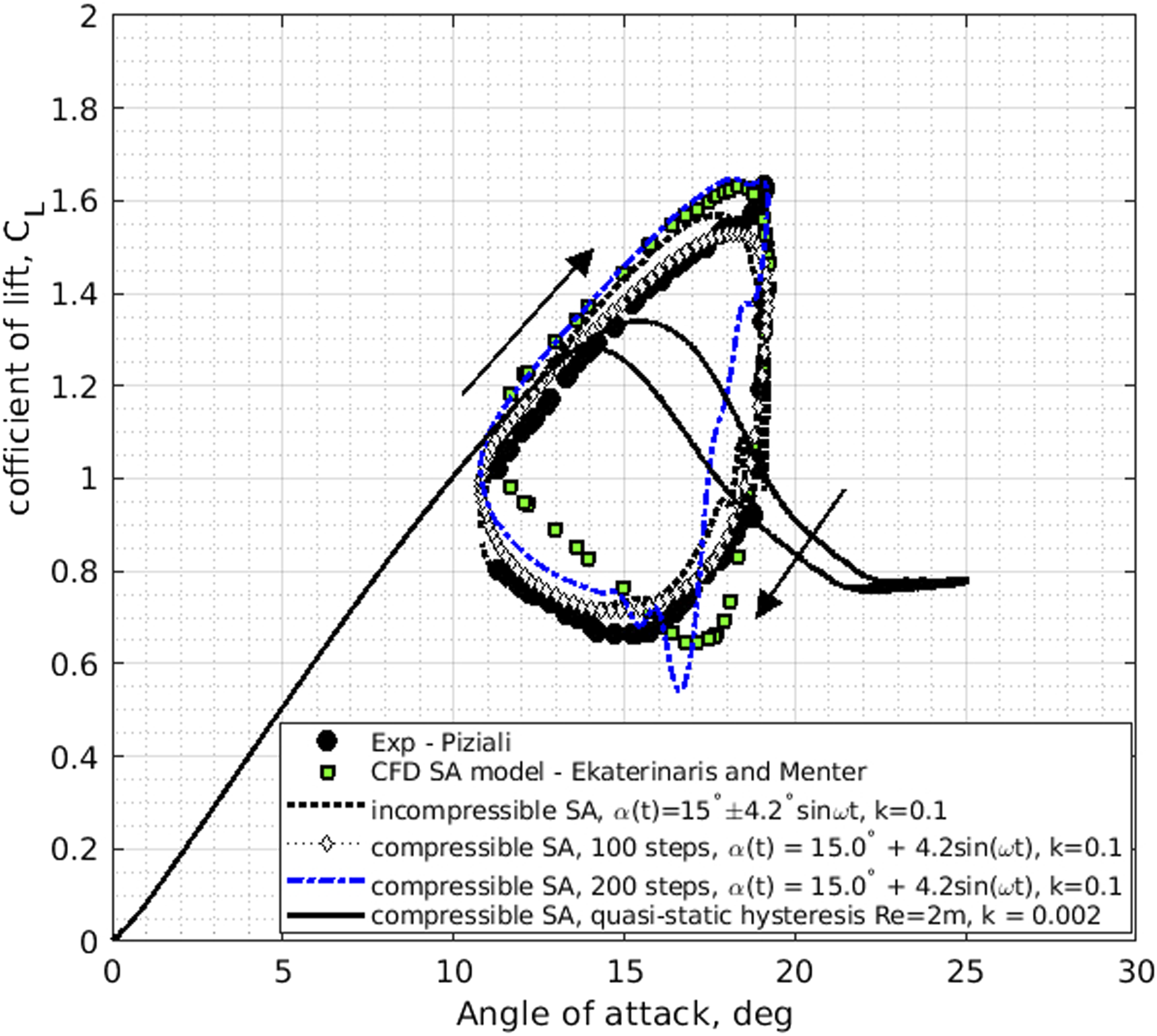
The OpenFOAM simulation results for quasi-static and dynamic hysteresis loops in the lift coefficient C_L along with prediction of the static dependence C_L(α) are shown in Figure 10. The simulation Reynolds number based on chord length is $Re=2.0\times {10}^6$ and Mach number in the free stream is $M=0.3$ . Initial CFD simulations involved testing the performance of the incompressible dual time solver against CFD and experimental results. On analysis of the obtained results from the incompressible solver, even with 200 steps in the pitch cycle and nearly 100−200 pseudo sub-cycles, the incompressible solver was not able to match the results against the published CFD results in Refs. 11 and 15 and the experimental results in Ref. 8 for the upstroke motion. This can be explained by relating to the contours of Mach number magnitude shown in Figure 11 obtained by the implemented compressible dual time solver. During the upstroke motion at $\alpha ={19.08}^{\circ }$ , the local Mach number magnitude on the upper surface of the airfoil close to the LE reaches the value of $M\ge 1.0$ . The local transonic/supersonic flow zone in the near vicinity of the LE causes changes in density and therefore the pressure distribution on the surface of the airfoil. Nevertheless, the incompressible flow solver generally gives arguably good results (black dashed line), especially during the downstroke motion where the changes in the local Mach number magnitude does not exceed critical compressibility regimes.

Figure 10.

Lift coefficient $C_L$ for the NACA 0015 airfoil in periodical motion $\alpha \left(t\right)={15}^{\circ }+{4.2}^{\circ }\hspace{0.17em}\mathit{sin}\left(\omega t\right)$ with $k=0.1$ , $Re=2\times {10}^6$ and $M=0.3$ , experimental results from Ref. 8.

Figure 11.

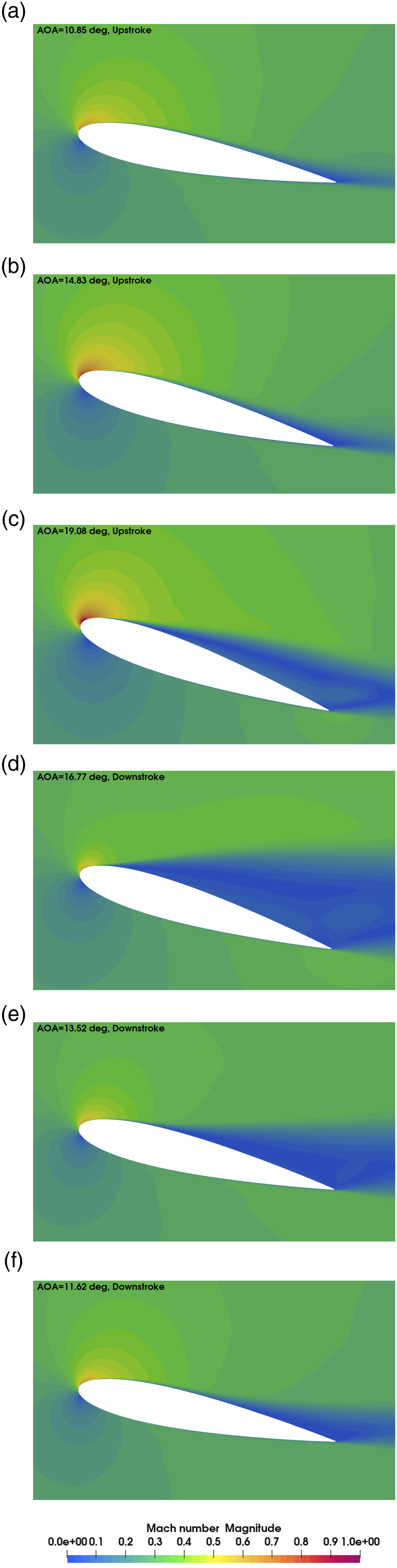
Contours of Mach number during pitch cycle with $\alpha \left(t\right)={15}^{\circ }+{4.2}^{\circ }\hspace{0.17em}\mathit{sin}\left(\omega t\right)$ , $k=0.1$ , $Re=2\times {10}^6$ and $M=0.3$ : (a) upstroke – $\alpha \left(t\right)={10.85}^{\circ }$ , (b) upstroke – $\alpha \left(t\right)={14.83}^{\circ }$ , (c) upstroke – $\alpha \left(t\right)={19.08}^{\circ }$ , (d) downstroke – $\alpha \left(t\right)={16.77}^{\circ }$ , (e) downstroke – $\alpha \left(t\right)={13.52}^{\circ }$ and (f) downstroke – $\alpha \left(t\right)={11.62}^{\circ }$ .

The comparison in Figure 10 also shows that using 100 time steps (white diamond markers) in the pitch cycle with the compressible solver is sufficient to resolve most of the flow characteristics and is in close agreement with the experimental results obtained in Ref. 8 during the majority of the upstroke motion and for the entire downstroke motion. The shedding of vortex during a finite small time interval is responsible for the sudden peak in the lift coefficient at $\alpha \approx {19.1}^{\circ }$ . Since 100 steps in pitch cycle did not capture this peak lift coefficient, the simulation was done again with 200 steps (blue dashed line Figure 10), and the upstroke C_L prediction improved significantly including the prediction of the peak C_L at $\alpha \approx {19.2}^{\circ }$ . The implemented dual time incompressible/compressible solver shows a good level of accuracy and usually requires just about 100–200 time steps per pitch cycle for capturing dynamic stall characteristics at high reduced frequencies.

Contours of the Mach number distribution in Figure 11 show that the upstroke motion is characterized by development of separation on the suction side which is nearly separated from the leading edge at $\alpha ={19.08}^{\circ }$ . On the downstroke motion, the flow is characterized with large separation zones even at a lower angle of attack of $\alpha ={11.62}^{\circ }$ . The quasi-static hysteresis results (black solid line) at reduced frequency of $k=0.002$ suggest that the maximum lift coefficient in nearly static conditions will be at $\alpha \approx {15}^{\circ }$ . The width of the quasi-static hysteresis loop in this case is quite significant $\mathrm{\Delta }\alpha \approx 6-7^{\circ }$ . It is quite physical to think that in the presence of hysteresis, if the dynamic stall centre point or the mean angle of attack is coincided with the centre of the static hysteresis and is given enough amplitude to cover the width of static hysteresis, the depth and size of the dynamic loops might amplify as the dynamic stall separation points $x_{se{p}_{dyn}}$ will form around the top and bottom branches quasi-static hysteresis separation points on the airfoil.

Case 3: Deep stall – NACA 0012 airfoil at $Re=0.135\times {10}^6$

Dynamic hysteresis for the NACA 0012 airfoil at moderately low Reynolds number of $Re=1.35\times {10}^5$ was simulated at low Mach number of $M=0.1$ with reduced frequency of $k=0.1$ . Oscillations of the angle of attack with an amplitude of ${\alpha }_m={15}^{\circ }$ around the mean angle of attack ${\alpha }_0={10}^{\circ }$ allow to cover the stall zone with fully separated flow conditions.

The flow regime in this case falls in the laminar turbulent transition zone at $Re=\mathrm{135,000}$ , and the use of a transitional model can be assumed to be advantageous. ¹¹ The experimental results used for comparison of this case are from Ref. 33 and it was concluded in this work that the LE dynamic stall was not associated with the bursting of the LSB, but with a sudden turbulent breakdown at a short distance downstream of the LE. ³³ Further to that, the work in this paper is mostly focused on capturing the global deep separated flow conditions and the overall trend with less computational resources; therefore, the SST turbulence model was considered as a compromising solution and used to predict the dynamic hysteresis loops.

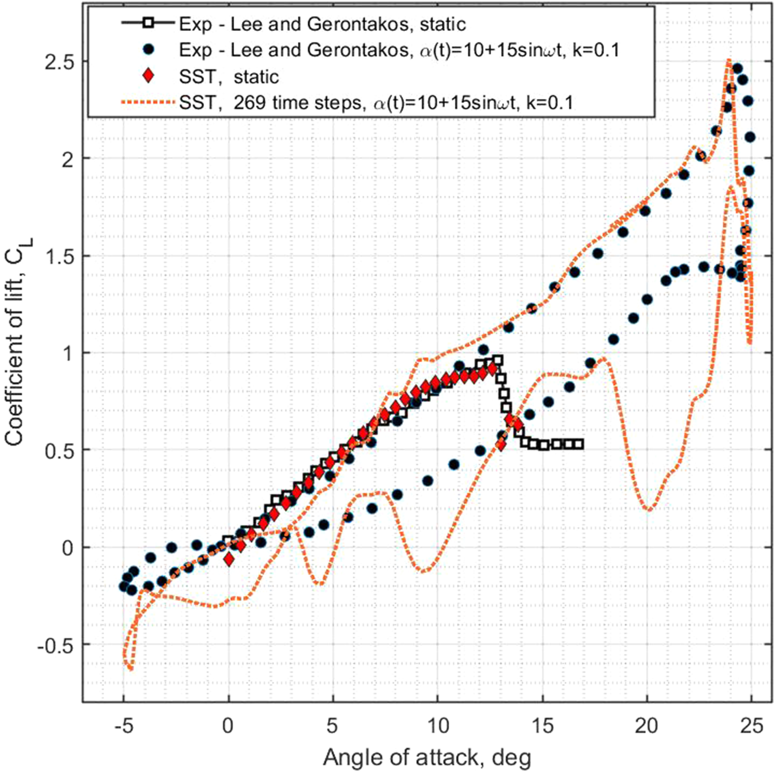
In Figure 12, the obtained simulation results are compared with the experimental data from Ref. 33. The computational results for the dynamic stall case shown in Figure 12 are in good agreement with the experimental results from Ref. 33. During the upstroke motion, the lift coefficient from the simulations (dashed orange line) is closely matching the experimental results, while the downstroke lift coefficient is predicted with reasonable accuracy. Note that most experimental results for dynamic stall are often filtered to remove high-frequency oscillations. Additionally, Figure 12 shows that the static lift coefficient from the conducted CFD simulations is also in good co-relation with experimental results including the stall angle.

Figure 12.

Lift coefficient $C_L$ for the NACA 0012 airfoil in sinusoidal motion, $\alpha \left(t\right)={10}^{\circ }+{15}^{\circ }\hspace{0.17em}\mathit{sin}\left(\omega t\right)$ , with $k=0.1$ , $Re=1.35\times {10}^5$ and $M=0.1$ (experimental results from Ref. 33).

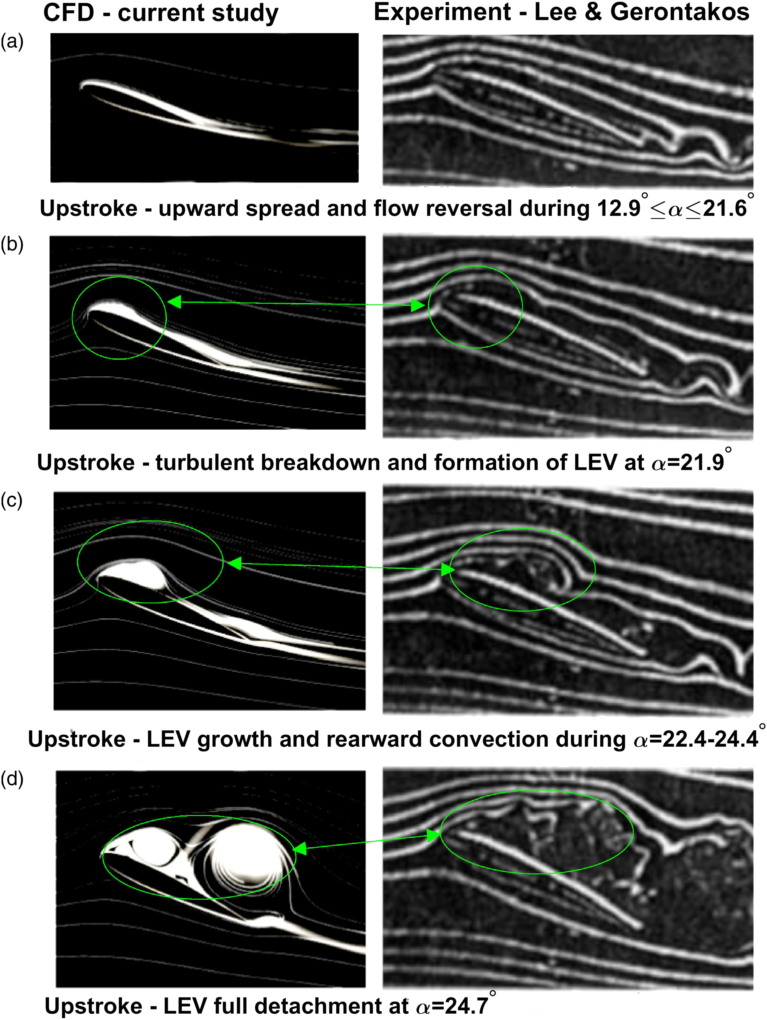
To better understand the flow processes during the dynamic hysteresis loop, streamlines of the velocity were superimposed on contours of vorticity to make meaningful comparison against experimental visualization for this case study presented in Ref. 33. Four distinct stages of the upstroke motion as described in the experiment are compared in Figure 13. In stage (a), attached flow conditions were noticed between angles of attack ${12.9}^{\circ }$ and ${21.6}^{\circ }$ , along with reversed flow from the trailing edge similar to experimental results. In stage (b), close to angle of attack $\alpha \approx {21.9}^{\circ }$ , the turbulent breakdown of the boundary along with formation of the LEV was shown in both experimental results and CFD simulations. Stage (c) showed the LEV growth and rearward convection which occurred between ${22.4}^{\circ }\ge \alpha \le {24.4}^{\circ }$ . Stage (d) with full detachment of the LEV occurs at $\alpha \approx {24.7}^{\circ }$ . The precise angle of attack instance at which the visualization was produced for each stage is shown in the caption of Figure 13. The simulation does not resolve all scales of turbulent eddies as shown in the experiment, and a pure large eddy simulation (LES) or a hybrid RANS-LES approach may be employed if this is of interest. However, the major events involved in the dynamic stall for this case described from stage (a) to stage (d) are captured accurately and at the same instance of angle of attack as shown in the experiment.

Figure 13.

Comparison of streamlines of velocity field superimposed on vorticity contours with experimental results during the upstroke motion for the pitch cycle $\alpha \left(t\right)={10}^{\circ }+{15}^{\circ }\hspace{0.17em}\mathit{sin}\left(\omega t\right)$ with $k=0.1$ , $Re=1.35\times {10}^5$ and $M=0.1$ (experimental results from Ref. 33) and CFD visualizations carried out at angle of attack: (a) $\alpha ={19.1}^{\circ }$ , (b) $\alpha ={21.9}^{\circ }$ , (c) $\alpha ={22.8}^{\circ }$ and (d) $\alpha ={24.7}^{\circ }$ .

Case 4: Quasi-static hysteresis stall – NACA 0018 airfoil at $Re=0.3\times {10}^6$

Experimental observations of static aerodynamic hysteresis on the NACA 0018 airfoil at $Re\approx 0.3\times {10}^6$ have been reported from a number of wind tunnel tests,^1,5,35 showing the presence of aerodynamic static hysteresis loops, but with different transitions between bi-stable flow structures. This can be explained by a high sensitivity of the experimental results to variations in the test conditions such as the level of free-stream turbulence, aero-elastic oscillations of a supporting rig and the adopted method for changing angle of attack.

Computational predictions of aerodynamic quasi-static hysteresis demonstrating bi-stable flow structures also have a high sensitivity to computational framework parameters similar to the experiment, while simulation of dynamic hysteresis is more robust to the setup of numerical framework. This is reflected by small number of successful computational predictions of the aerodynamic hysteresis reported in the literature.^3,5,6

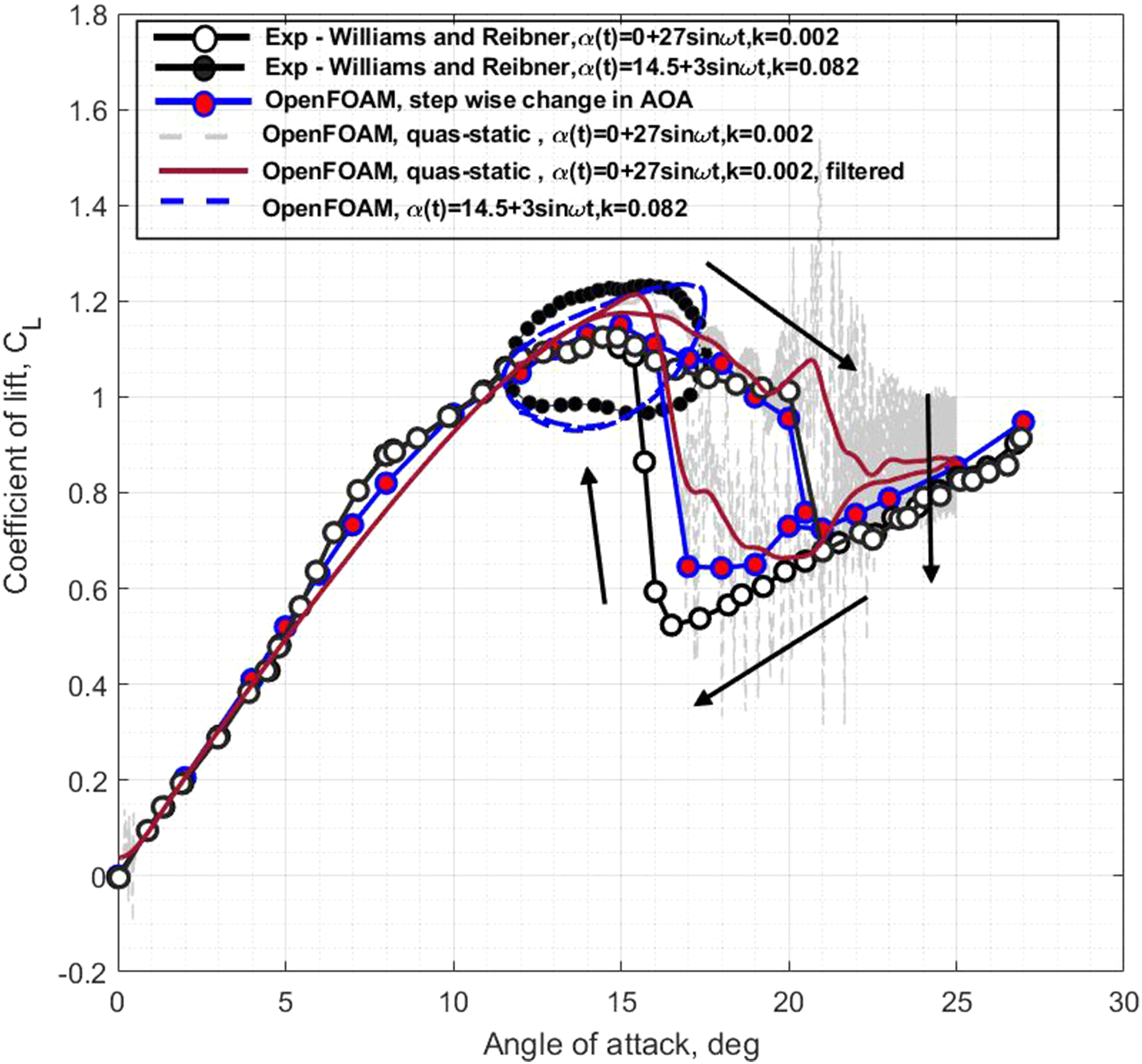
Figure 14 shows that the OpenFOAM simulation results obtained as stationary solutions of the RANS equations with the SST turbulence model in Ref. 5 are quite accurately matching the experimental data from Ref. 1 showing the hysteresis dependence in the lift coefficient of the NACA 0018 airfoil. Both computational and experimental data are obtained at $Re=0.3\times {10}^6$ .

Figure 14.

Lift coefficient $C_L$ for NACA 0018 for quasi-static and dynamic stall hysteresis at $Re=0.3\times {10}^6$ and $M=0.013$ .

One can expect that the same quasi-static hysteresis loop can be obtained in a very slow variation of angle of attack with upstroke and downstroke motions using the URANS-SST equations. The slow variation of the angle of attack was implemented in the form $\alpha \left(t\right)=0^{\circ }+{25}^{\circ }\hspace{0.17em}\mathit{sin}\left(\omega t\right)$ with reduced frequency $k=0.002$ . This kinematics limits the rate of change of angle of attack as $\left|\alpha \dot{}\right|\le 0.5-1.0\mathit{deg}/s$ . The unsteady solution of the URANS-SST equations was obtained using the implemented DTS method, which significantly saved CPU simulation time. In this case, the obtained variation of the lift coefficient C _L is shown in Figure 14 with light grey line, and the filtered process for C ^filt _L is shown with dark red line.

During the upstroke motion, the simulated lift coefficient shows good agreement up to the maximum lift coefficient CL_max with the experimental dependence from Ref. 1 and also with the simulation results in static conditions from Ref. 5. The low rate of change in the angle of attack does not cause a dynamic overshoot in the lift coefficient, and this is a good indication that simulation results are close to their quasi-static values. The quasi-static hysteresis results show the onset of a buffet at $\alpha \ge {18}^{\circ }$ , although the wind tunnel test results do not show any signs of buffeting probably due to averaging procedures applied. With the applied filtering process, the observed hysteresis loop in the OpenFOAM simulation is almost as wide and deep as in the CFD predictions in Ref. 5 and experimental results from Refs. 1 and 2.

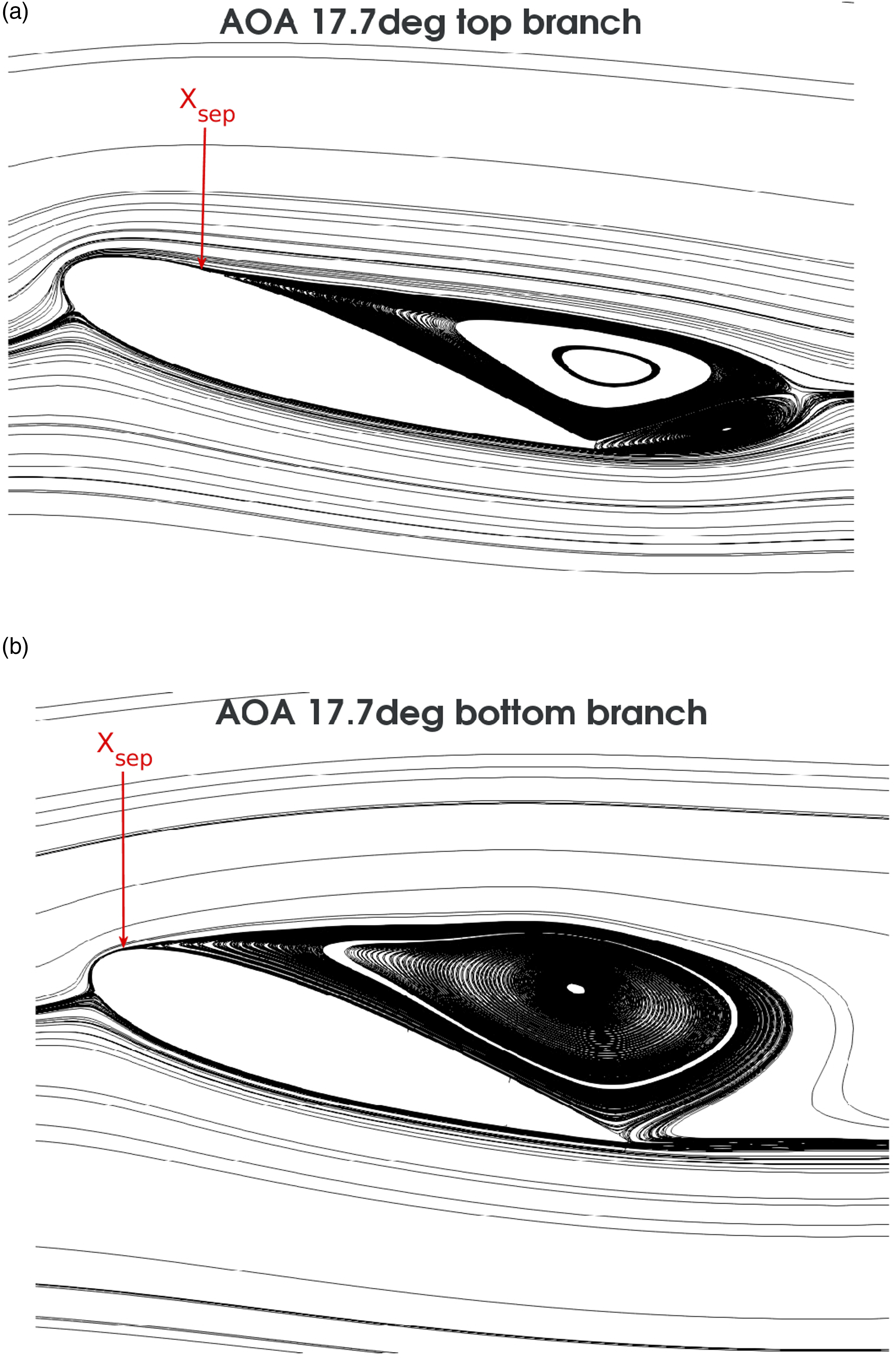
Figure 15 shows flow patterns with separated circulatory zones visualized by streamlines for the upper and lower branches of hysteresis loop at the same angle of attack $\alpha ={17.7}^{\circ }$ .

Figure 15.

Projected streamlines of flow for the NACA 0018 airfoil at the same angle of attack during quasi-static hysteresis: (a) top branch, $\alpha ={17.7}^{\circ }$ , and (b) bottom branch, $\alpha ={17.7}^{\circ }$ .

The flow separation points $X_{sep}$ shown in Figure 15 illustrate that on the upper branch of hysteresis the flow remains attached over the leading quarter of the airfoil, while on the bottom branch of quasi-static hysteresis loop the flow separates from the LE of the airfoil. This difference in location of separation points leads to a significant drop in the lift coefficient.

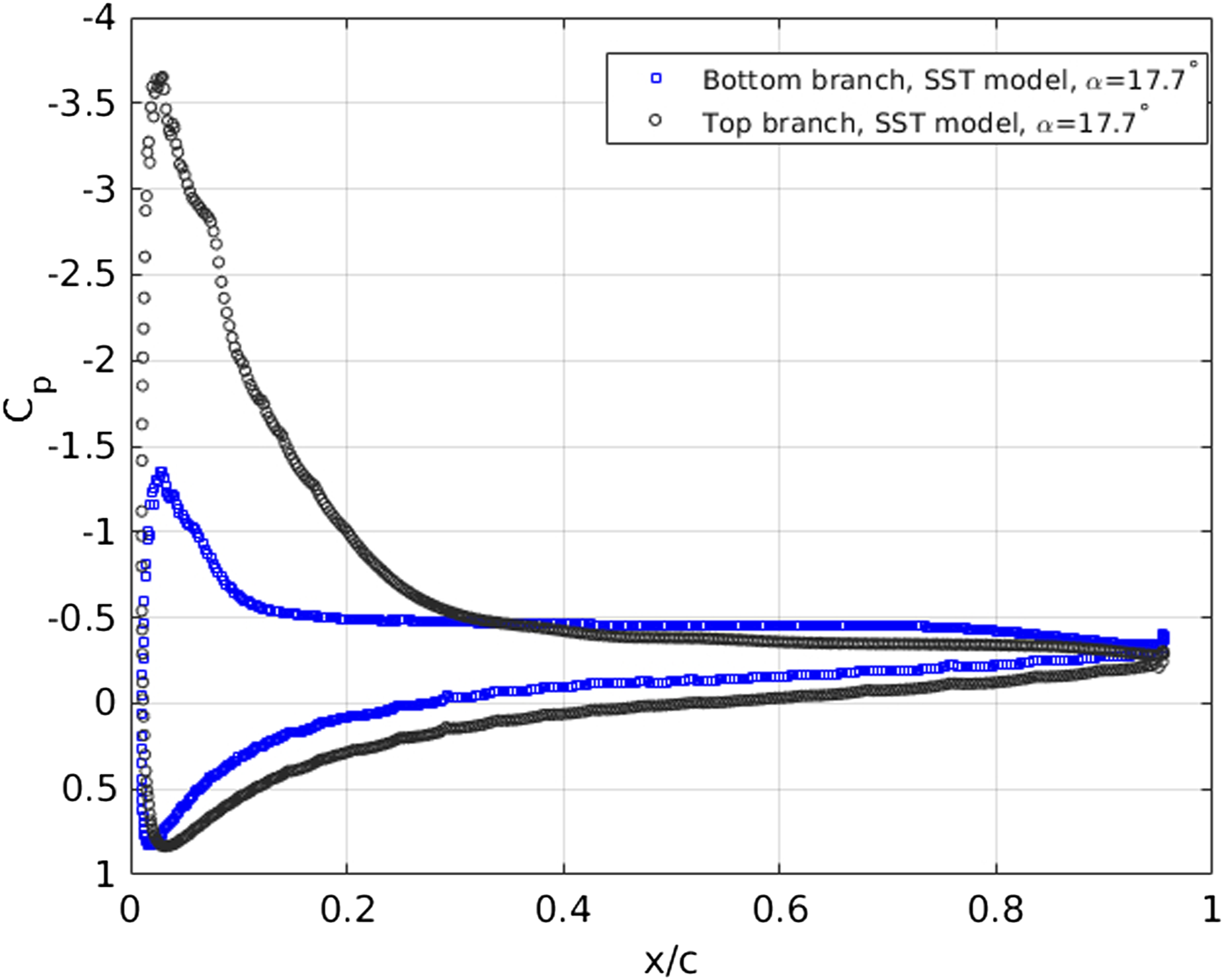
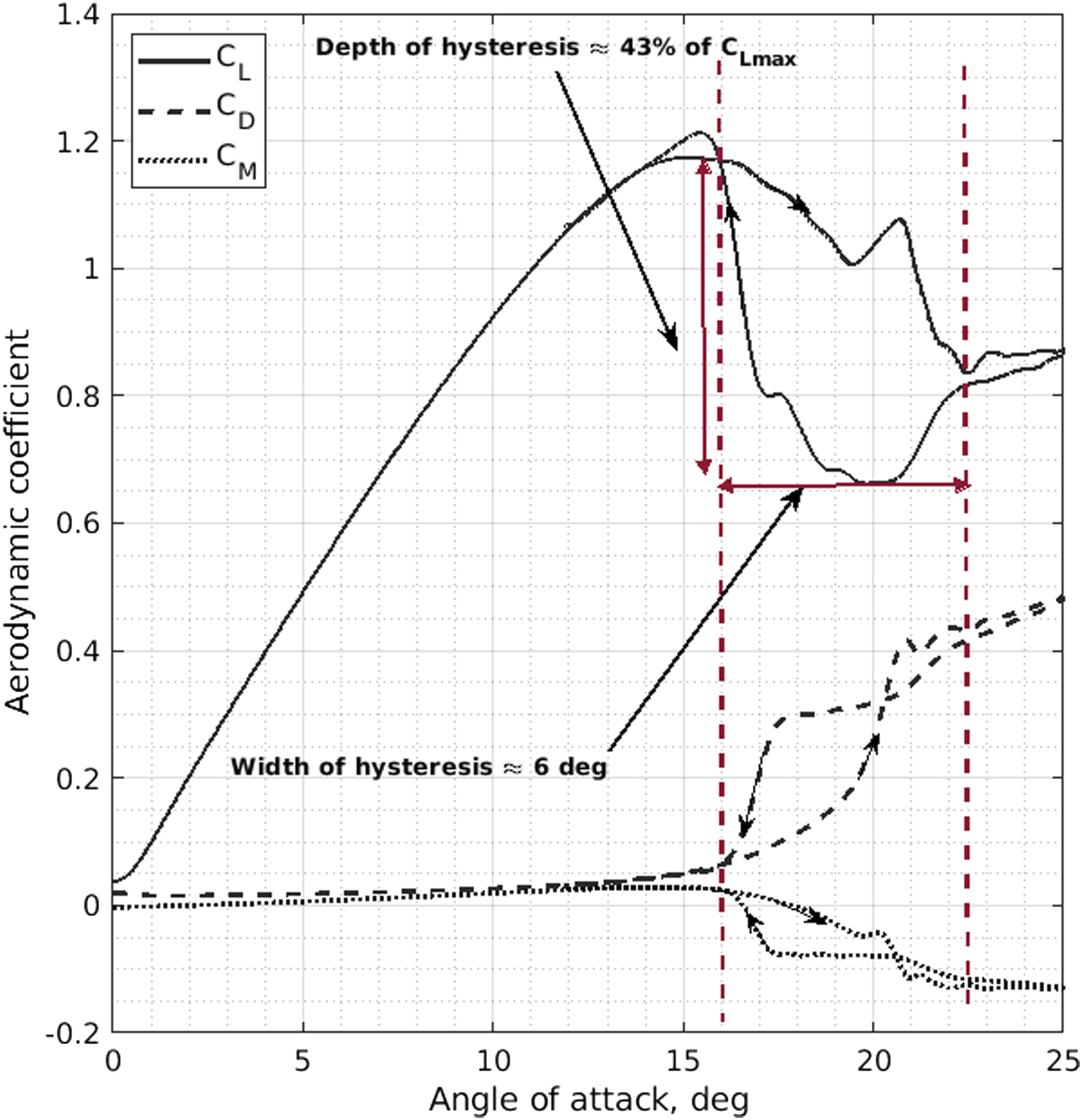
The distributions of the pressure coefficient C _p (x) for the two branches of quasi-static hysteresis in Figure 16 show that the reduction in the lift coefficient C_L on the bottom branch of quasi-static hysteresis is due to significant loss of the pressure coefficient over the first quarter of the airfoil suction side. The averaged variations of lift, drag and pitching moment coefficients $C_L,C\_D$ and $C_M$ in Figure 17 clearly show the presence of hysteresis loops in aerodynamic coefficients.

Figure 16.

Pressure coefficient $C_p$ distribution for the NACA 0018 airfoil at the same angle of attack $\alpha ={17.7}^{\circ }$ on the top and bottom branches of quasi-static hysteresis.

Figure 17.

Results obtained for hysteresis in the aerodynamic coefficients of NACA 0018 airfoil at $k=0.002$ and $Re=0.3\times {10}^6$ .

Conclusions

The implementation in OpenFOAM of a computationally stable and robust DTS method for pressure-based incompressible flow solvers, in combination with segregated solver methods such as the SIMPLE, has made it possible to investigate and validate the phenomena of aerodynamic quasi-static and dynamic stall hysteresis for a wide range of Reynolds numbers with significant savings in CPU time, for example, simulations of dynamic hysteresis loops are about 20 times faster than when using pimpleFoam solver.

Overall, the simulation results are in good agreement with the available wind tunnel data as well as published CFD simulation results, showing that the adopted computational framework with lower computational requirements is suitable for studying hysteresis phenomena in the stall zone. The improved solver is planned to be used to determine the delay and relaxation time scales in a nonlinear phenomenological model of quasi-static and dynamic stall hysteresis of various types of airfoils at various Reynolds numbers.

The sensitivity of quasi-static hysteresis in computer simulations to the choice of the time integration method, the level of free-stream turbulence and the spatial discretization of the grid requires further study.