
Abstract
A novel quasi-dynamic guidance law (QDGL) is presented for a dual-spin projectile (DSP) with unconventional constraints on roll direction. A 7 degree-of-freedom (DOF) dynamic model is established and the projectile operational mechanism is presented with a description of how it is used to enact control. The QDGL is presented and a parametric study is conducted to show how the QDGL parameters affect the system response. A procedure of using batches of Monte Carlo simulations is described, to numerically compare the system response with different QDGL configurations. A genetic algorithm is then used to optimise both the innate system parameters and PID controller gains. The disturbance rejection capabilities of the optimal QDGL are then evaluated along with the performance against different target profiles. It was found that the GA optimised QDGL is able to provide satisfactory control capabilities against static and dynamic targets.
Introduction
The calibre of guided weapons is getting ever smaller to meet the evolving needs of modern engagement scenarios. This is in turn driving a reduction of critical subsystem volumes of guidance and control hardware. It is thus pertinent to develop a novel method of control so as to either minimise the necessary subsystems occupying a volume or reduce the demand on subsystems/materials which are included in the projectile. This would allow a reduction in calibre with currently available technology without having to advance the capabilities of any specific subsystem/material.
Dual-spin projectiles (DSPs), such as STARSTREAK, 1 are becoming more prevalent in today’s military arsenals as they enable a wide scope of target engagement profiles. The dual-spin configuration slows the roll rate of the forward section to a point where the response rate of the actuators is sufficiently high compared to their roll rate such that effective control can be enacted. The aft section stays at the high roll rate and the projectile thus maintains gyroscopic stability. Guidance modules in the form of course corrected fuses are also being retrofitted onto conventional munitions, such as the Orbital ATK Armament Systems’ M1156 Precision Guidance Kit 2 and BAE’s Silver Bullet. 3 In these larger weapon systems (155 mm), the roll rate of the projectiles is relatively low compared to smaller calibres. For smaller projectile calibres with high roll rates, it may not prove feasible to mitigate the high roll rates to apply conventional control methods.
Some prevalent examples of conventional guidance laws (GLs) used in projectiles include proportional navigation (PN), proportional derivative (PD) and sliding mode control (SMC). 4 Conventional SMC or variations thereof have already considered constraints such as autopilot lag and actuator fault, 5 accelerator saturation, 6 and modelling uncertainty in missile/target dynamics. Impact angle is often the considered an aspect for control in a GL. In addition to purely controlling the impact angle, 7 secondary constraints have also been placed on trajectory time, 8 field-of-view,9–11 and manoeuvrability. 12 External uncertainties and missile jerk have also been considered. 13
A modified SMC GL was used to improve the chattering, miss-distance and finite time over conventional SMC and PN methods. 14 The validity of the PN-like LOS GL has been investigated for a three body (two aircraft, one missile) system where the launch platform is also moving. 15 A novel variation, called ‘airborne-CLOS’ utilises two separate LOS rates with one gain to control the three body problem. 16
A novel GL has been created utilising virtual targets for impact angle and burst height constraints. 17 A polar GL has been investigated which controls a missile based on the polar radius and angle of the target from the missile. 18 An expanded 2D PD GL was created for a skid-to-turn command to LOS anti-tank guided missile, which builds upon classic PD, with the objective of eliminating a spiral trajectory which is an artefact of PD GLs. 19 A proposed method uses a weighted zero-effort-miss (ZEM) to shape the actual ZEM, presenting as a PN GL with an extra time varying gain.
A few publications specifically pertain to the guidance of DSPs. Iterative impact point prediction has been used to create a GL for a DSP with control force imparted by fixed canards 20 . A modified form of projectile linear theory is used to predict where the projectile will land and make the necessary corrections to the control system. Proportional navigation has been used in the GL of a dual-spin mortar during the ascent and descent phase. 21 The results of the GL were validated with hardware-in-the-loop testing and Monte Carlo simulations.
It is a common practice to neglect gravitational forces when creating a GL.22–25 Once an idealistic GL has been created, constraints can then be placed on the model which reflect conditions present in chosen real-world systems. GLs are often described from the perspective of the YZ plane (shown in Figure 1) also known as the ‘picture plane’.7,18,19 Some of the cited literature use kinematic models for the derivation and validation of the control law,8,12,14,15,17 while this paper uses a dynamic projectile model. It is common to test the GL using arbitrary model parameters to facilitate more efficient and reliable interpretation of the results.18,19 Dual-spin projectile with fixed control force F
c
.
Conventional projectile control utilises control surfaces which are able to adjust the roll angle of a projectile as well as the magnitude of the control force. The conventional guidance strategy is to roll the projectile to align the controllable pitch axis with the desired direction, and then increase the force by actuating the control surfaces which results in lateral movement. Dual-spin projectiles use a similar method with the addition of a coaxial motor to assist the correction of the forward section roll angle. 26 This paper proposes a quasi-dynamic GL (QDGL) for a DSP, with a fixed roll direction as well and a fixed magnitude control force; however, the phase of the force can change, hence the quasi nature. Control is enacted by adjusting the roll rate of the control force, slowing it down through certain roll angles to bias the force in the desired direction. There currently exists no literature which describes a GL for a DSP with roll-direction, roll-rate and control-force magnitude constraints.
The section Projectile Dynamics describes the 7 degree-of-freedom (DOF) dynamic model of the projectile used in simulations. The section Quasi-dynamic guidance law formulation introduces the projectile design and describes how control is enacted with the asymmetric roll constraints. The QDGL and associated parameters are introduced, with a brief parametric investigation showing their effect on the system response. The section Monte Carlo Procedure and Normalised Errors presents a Monte Carlo procedure which is used to numerically compare the effect that different QDGL configurations have on the system response. A genetic algorithm is then run to optimise the QDGL parameters as well as the gains of a PID controller. The system response of the optimised QDGL is evaluated against various disturbances and target profiles. The final section gives a summary of the paper and the key findings.
Projectile dynamics
This section describes the seven DOF dynamic model of the DSP, which has previously been used to investigate DSPs21,27–29 and is a derivative of the well-established model for a conventional projectile used by McCoy.
30
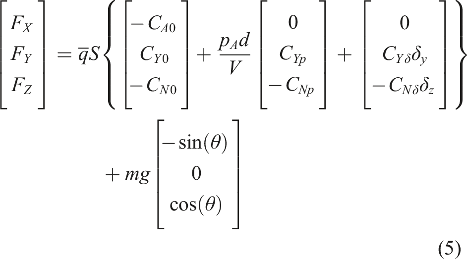
Subscript F denotes the forward section and subscript A denotes the aft section. The assumption is made that the total centre of mass (COM) coincides with the aft COM, that is, the mass of the forward part is small with respect to that of the aft part and the nose moment of inertia Ixx,F is small compared to the aft one Ixx,A. The forces and moments the projectile is subject to are represented by an aerodynamic coefficient. The whole body longitudinal CA0, transverse CY0 and normal CN0 coefficients represent the combined effect of these individual forces, and are shown in Figure 2 for non-zero angles of attack α. Projectile coefficients when α ≠ 0.
The non-linear kinematic translational and rotational equations are given by equations (1) and (2), respectively
Accordingly, the dynamic translational is shown in equation (3)
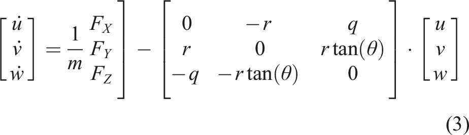
Here, the forces
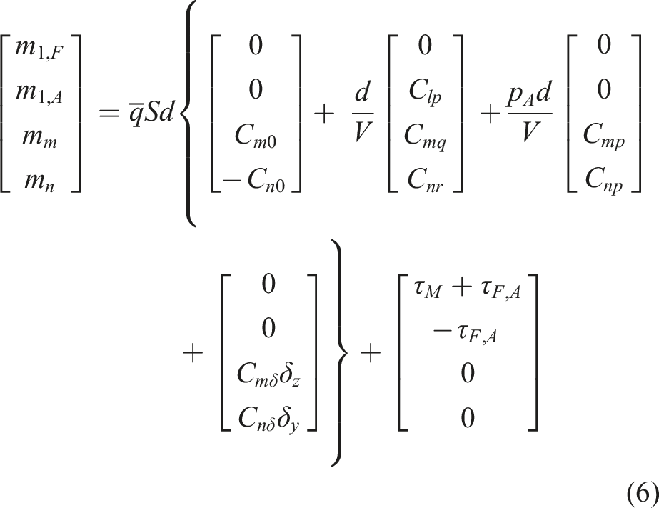
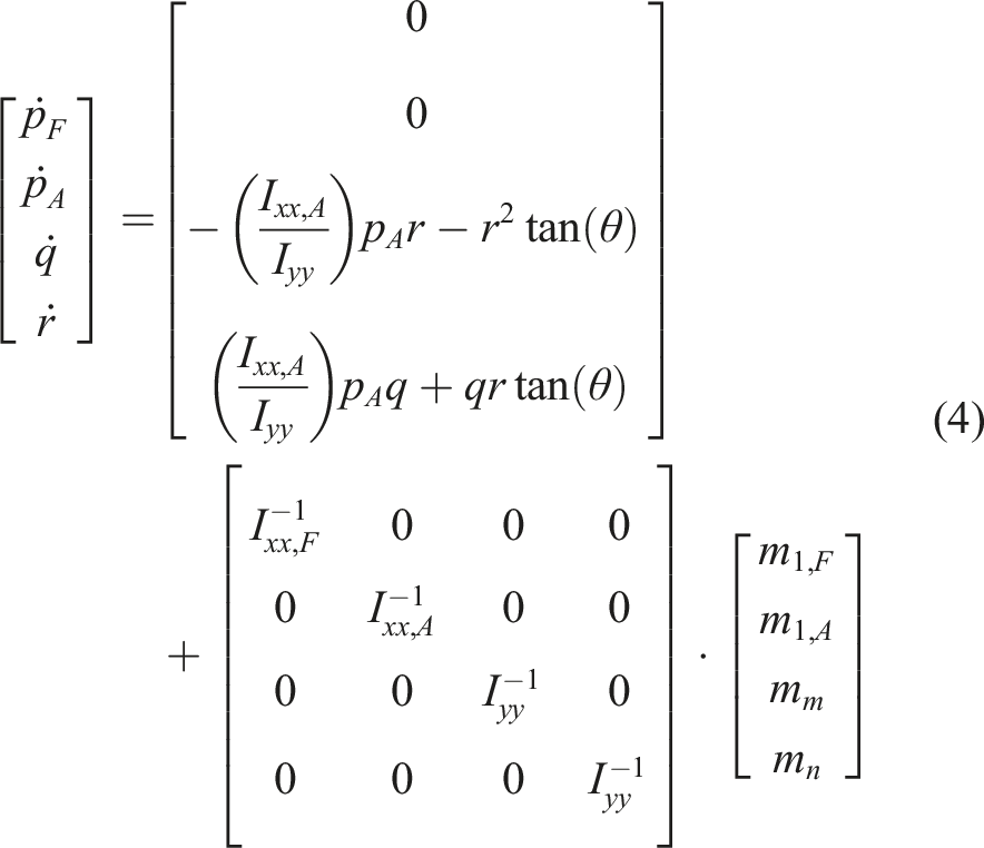
Here,
Quasi-dynamic guidance law formulation
This section describes the control method of the DSP design with unconventional roll constraints. The QDGL is formulated and the resulting system response is shown. A brief parametric study is conducted to illustrate how the QDGL parameters affect the system response.
Most guided projectiles have fins which can roll the projectile and induce a variable control force along a pitching axis. If lateral deflection is required, the projectile adjusts its roll angle such that the axis of the control force is parallel to the direction of required travel, whereby it increases the control force and therefore imparts an acceleration. Figure 3 shows the DSP design; a control force F
c
is produced by aerodynamic lifting surfaces on the forward section. At launch, the aft section engages with the rifling which accelerates the roll rate, while the forward section producing F
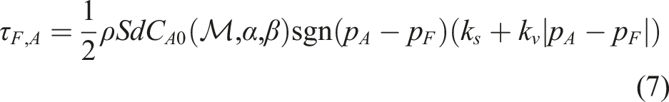
c
remains de-spun. During flight, the two sections will reach an equilibrium through the bearing torque τF,A, and the forward section will have a relatively slow roll rate, ω0. If τF,A is increased during flight (e.g. by means of a brake) then there will be new equilibrium where the forward section has a higher roll rate, ω1. Earth axis perspective of the picture plane and control force F
c
rotating at rate ω1 through angle ϕ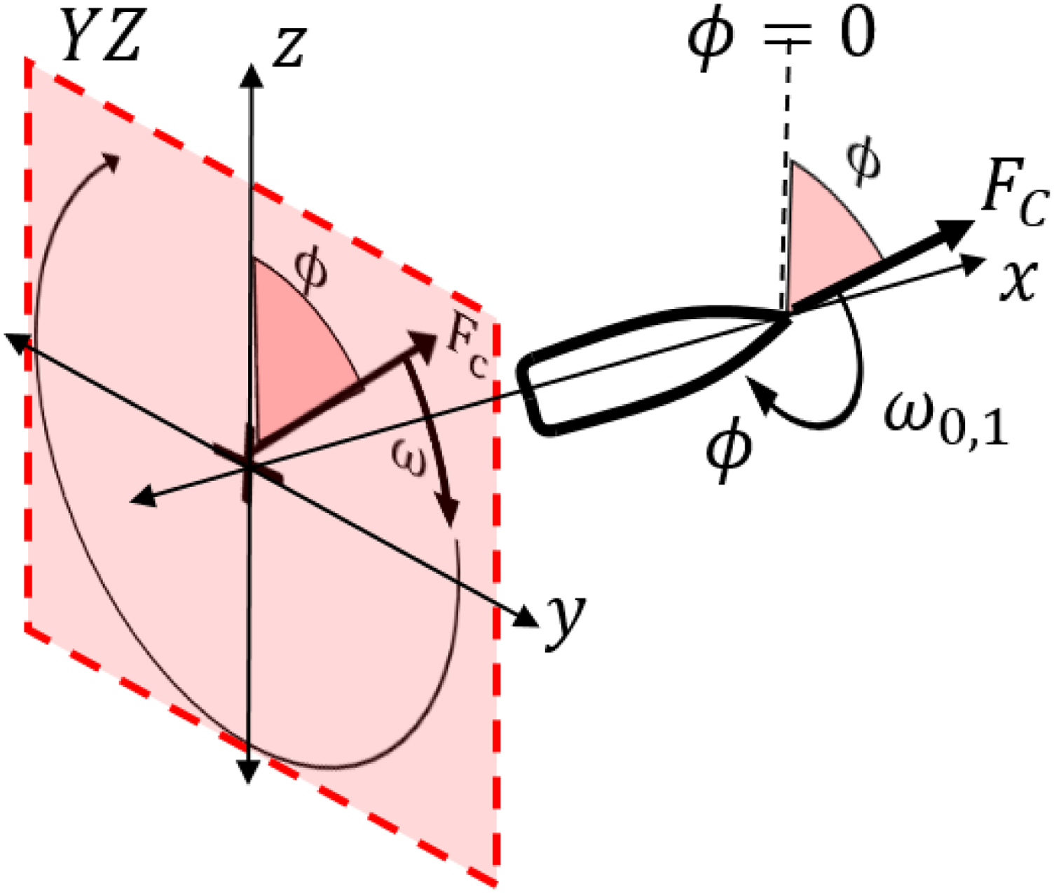
Figure 3 shows the key parameters of the control method, as well as the YZ plane, referred to as the picture plane. The constant magnitude F c moves through a roll angle ϕ with rate ω0 or ω1, where ω0 < ω1. The ϕ ∈ [0, 2π] describes the roll orientation of F c with respect to the normal axis. It sweeps in the negative mathematical direction, since most conventional projectiles have a right hand twist. The novel guidance strategy proposed herein uses a fixed magnitude F c rolling at speed ω1. The roll rate is slowed to ω0 through favourable roll angles when F c is aligned with the desired correction axis, and then accelerated back to ω1 through the remaining unfavourable roll angles. The act of slowing F c when sweeping through favourable roll angles is henceforth referred to as a ‘bias’. All measurements and symbols henceforth are given in the ‘picture plane’ reference frame unless explicitly stated.
The integral of Newton’s second law relates the impulse of an object, J, to its change in velocity Δv

Here, the mass is an assumed constant since there are no on-board resources being consumed. A generalised decomposition of F
c
onto any orthonormal axis i, j in the YZ plane has the corresponding forces F
i
, F
j
. Let the desired decomposition axis i be an angle ϕ
B
from the normal axis
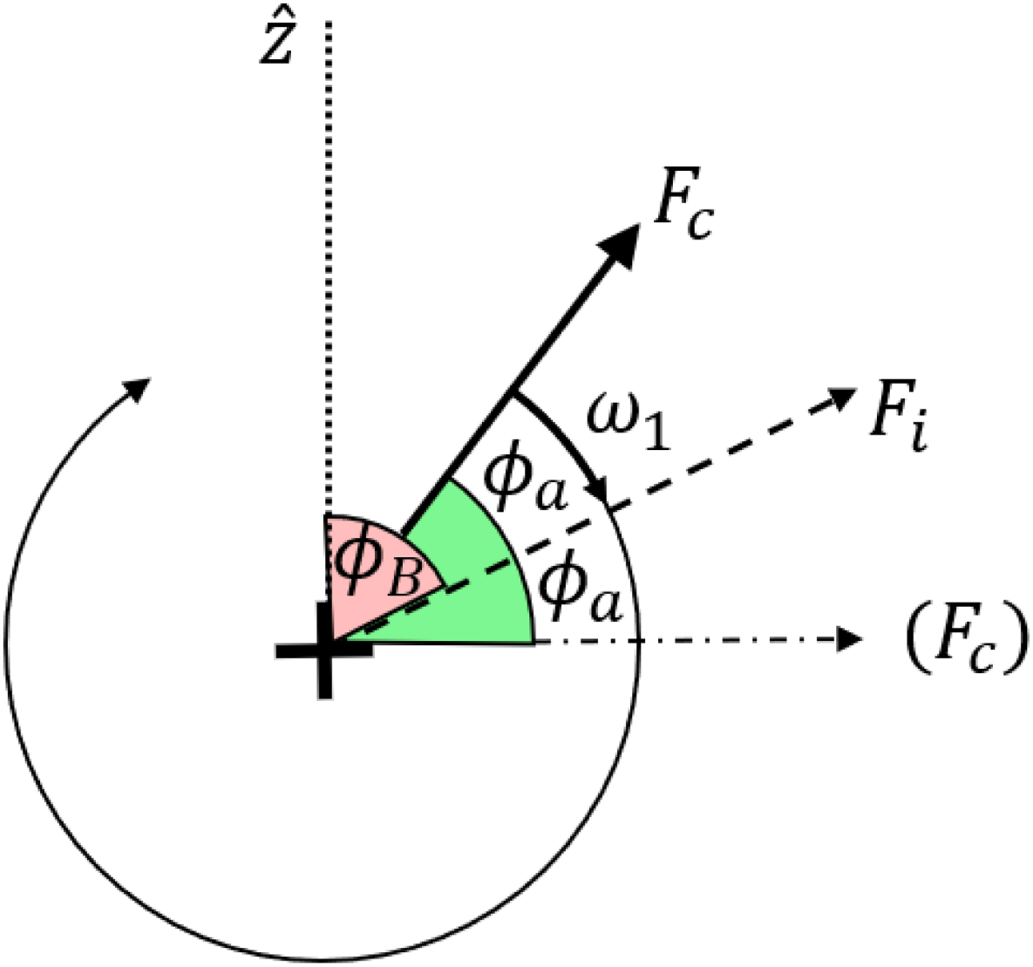
The range of angles during which F
c
is slowed is defined as the bias angle. Let the midpoint of the bias angle coincide with decomposition axis i, such that the symmetrical angle on either side of the midpoint is ϕ
a
. The bias angle thus starts at (ϕ
B
− ϕ
a
) and ends at (ϕ
B
+ ϕ
a
) with a midpoint of ϕ
B
. This is shown in Figure 4. However, F
c
will continue to rotate through the rest of the angle ϕ eventually sweeping another angular range (ϕ
B
+ π) ± ϕ
a
(wrapped so ϕ ∈ [0, 2π]). During this time, the resulting change in velocity is directed along the negative i
th
axis. Bias manoeuvre of size ϕ
a
centred about ϕ
B
.
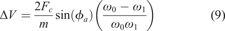
We define ΔV as the total change in velocity of one whole roll rotation in sweeping through equal but opposing angles of size 2ϕ
a
, at different rates ω0 and ω1. Assuming F
c
, m and ω as constants, it can be shown from equation (8) that

Comparison of simulation parameters used against real-world projectiles.
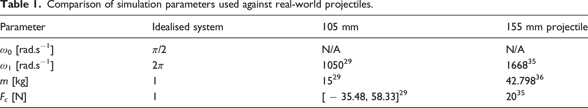
Since the purpose of this paper is to test whether the uni-rotational, fixed magnitude control force can be used to guide a projectile in the 2D plane, all forces and moments except the control force are neglected. Additionally, there is no transient between the fast and slow oscillations, and the switching is instantaneous.
By design, the QDGL calculates a desired change in speed when ϕ = 0, and then calculates the bias angles from equation (9). The projectile will then continue to roll, whereby the actuator will slow the roll down if the current roll angle lies within the bias range previously calculated. In practice, the desired speed change and resulting bias angles are calculated when ϕ lies in a small range, ϕ ∈ [0, 0.001], to account for the machine computation inaccuracy. While this calculation could be conducted and updated continuously, the relative speeds would have to be transformed to the ϕ = 0 reference frame which adds another layer of computational complexity. In addition, this discrete computation of speeds at the beginning of each rotation accommodates the bandwidth of hardware with respect to the roll rate of the projectile.
The current relative velocity of the projectile to target is the difference between the projectile and target velocity, V
R
= V − V
T
, or in full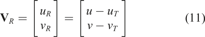
N.B. The projectile having [u0, v0] = [0, 0] and undergoing consecutive unbiased rotations does not result in a circular trajectory; instead a semi-circular trajectory would result. To achieve a circular trajectory in the resting state, the horizontal velocity at the beginning of the bias calculation must assume the control force has already rotated through one quarter rotation. Taking this into consideration, we define VDR0 as the ΔV correction necessary to bring the projectile to a stable circular orbit relative to the target, including the current relative velocity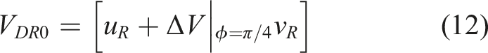
This only allows the autopilot to bring the projectile to relative rest, the desired closing speed V
PT
(d) describes the chosen approach speed as a function of d. The total demanded velocity change from the velocity autopilot V
Dem
is then a linear combination of the necessary relative speed correction to bring the system to an orbit, VDR0, and the closing velocity V
PT
(d) dictated by the QDGL is
V
PT
(d) must only demand speeds which can be delivered by the actuation mechanism, given that ΔV can never exceed ΔVmax. Let the function Vlim(d) be the maximum relative speed the projectile can have at a distance d ≥ 0, such that it is still able to decelerate in time to be at relative rest when d = 0. This function can be calculated by starting with a stationary projectile and applying consecutive ΔVmax biases, since the process is reversible. From the rates given by the idealised system parameters in Table 1, a ΔVmax = 0.954 9 ms−1 bias is enacted by the projectile in 2.5s. An effective acceleration value, 
Since the function V
PT
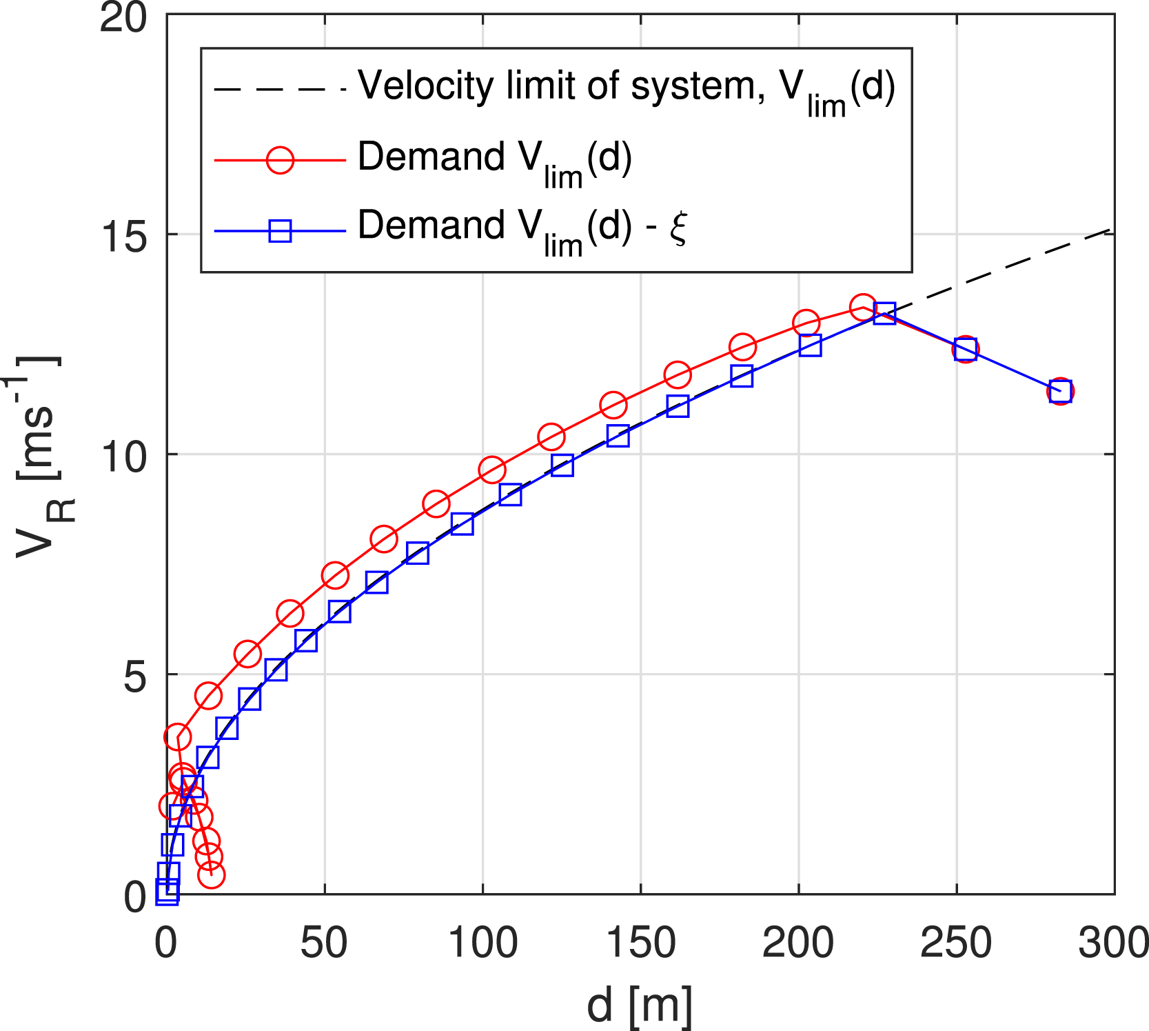
(d) is calculated when ϕ = 0 at a particular distance d1, the desired ΔV will not be achieved until after the bias manoeuvre has been executed one full rotation later. Hence, the process is discontinuous. By this point, the projectile will have moved to some new distance d2 under its residual velocity. Figure 5 shows the delay of the system response when the target speed is set to be the limit of the system, for example,. V
PT
(d) = Vlim(d). The data points indicate specific positions where ϕ = 0, triggering the calculation of the bias angles. Figure 5 illustrates how the value of Vlim(d) demanded at a specific point is achieved at the next calculation point but after the delay caused by the roll rotation. This delay causes the system to exceed Vlim(d), resulting in an overshoot. To account for the delay, the demanded speed is modified by a factor ξ which ensures the relative speed never exceeds Vlim(d). The delay does not directly scale with distance but rather with V
PT
(d) as it is the result of dynamic system evolution. Hence, the closing speed function is written as Effect of ξ to prevent system response exceeding Vlim(d).
By including ξ, V
PT
(d) is not properly defined when d ≤ d1 where d1| (V
PT
(d1) − ξ = 0). From equation (14), this boundary is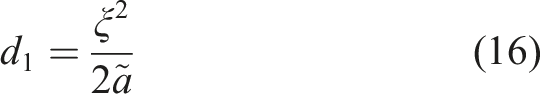
As such, the function Vlim(d) − ξ is only valid for d ∈ (d1, ∞] and must be defined by other means for d ∈ [0, d1]. Firstly, the distance d2 is chosen to represent the desired level of precision for the projectile. The projectile will remain relatively stationary within this threshold, when it is on course to hit the target, so V
PT
(d) = 0 ∀ d ∈ [0, d2] where 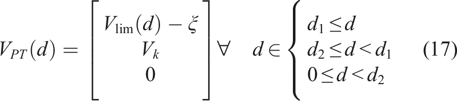
Monte Carlo Procedure and Normalised Errors
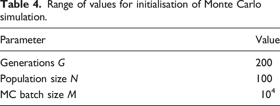
Range of values for initialisation of Monte Carlo simulation.
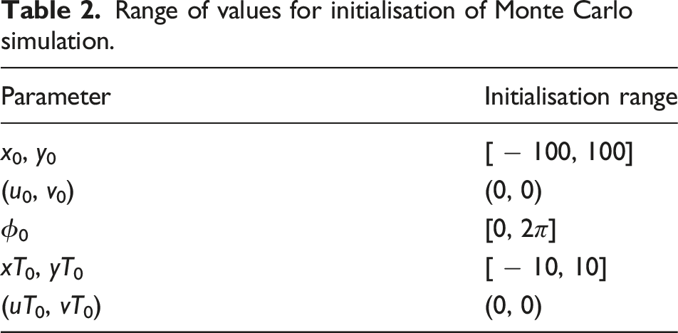
Multiple MCSs are run in a ‘batch’. Figure 6 shows the average system responses for four batches of 104 MCSs. The difference in the response is caused by the stochastic nature of the MCS initialisation. Increasing the batch size results in an average system response which is sampled over a large number of simulations, providing more consistency between batches as well as being more representative of the true system behaviour. Obviously, the maximum discrepancy between multiple batches is inversely proportional to the batch size. Response discrepancy between multiple batches of 104 MCSs.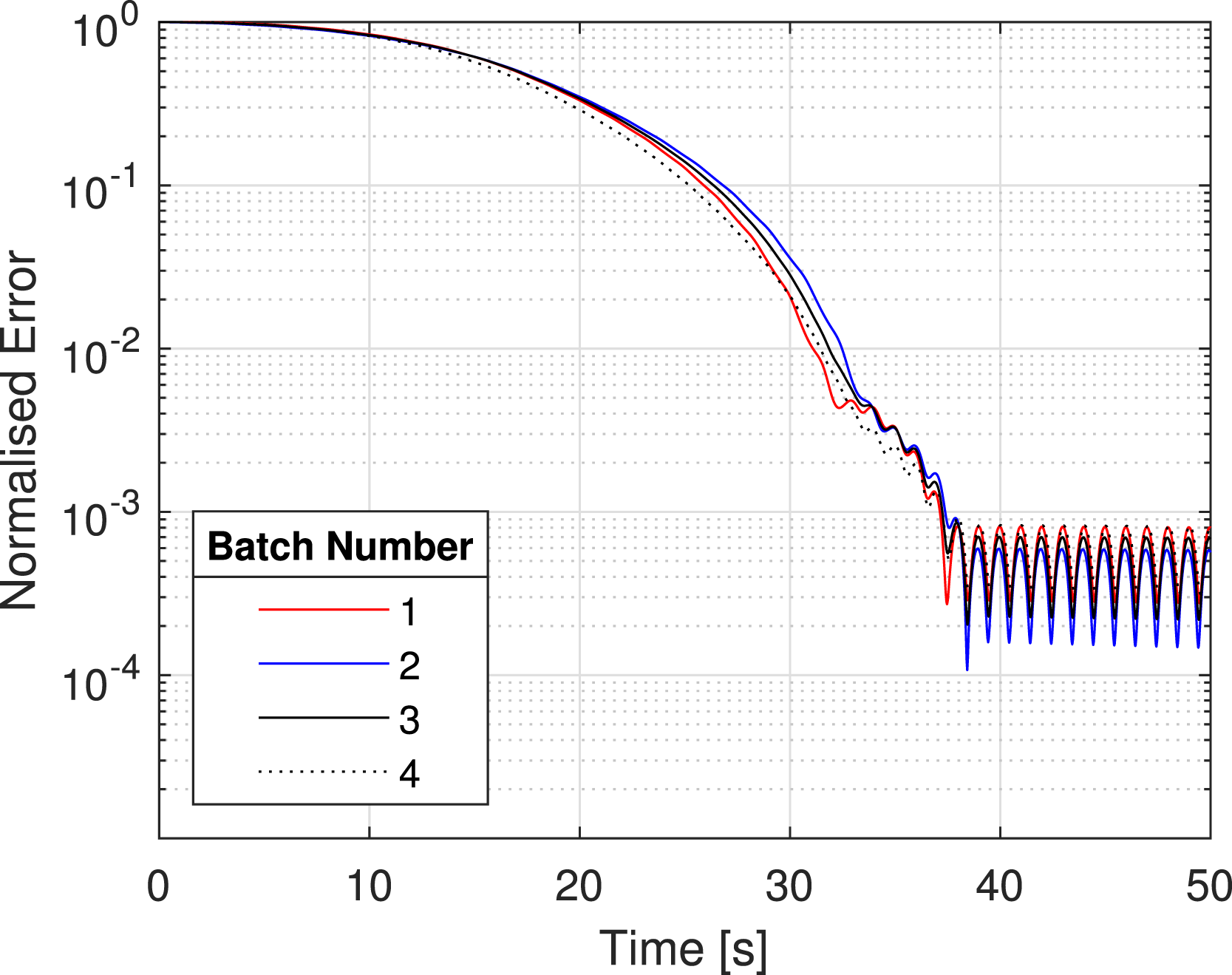
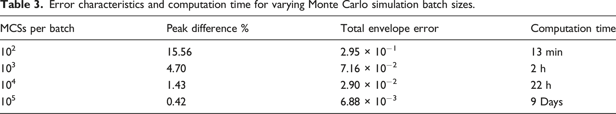
Figure 7 shows the instantaneous maximum error for varying batch sizes over time. For a given batch size, four separate batches are run. The maximum discrepancy between any of the four batches at any specific instances is plotted, for duration of the simulations. This process is repeated for four different batch sizes. Instantaneous maximum variation of the normalised error of different batch sizes.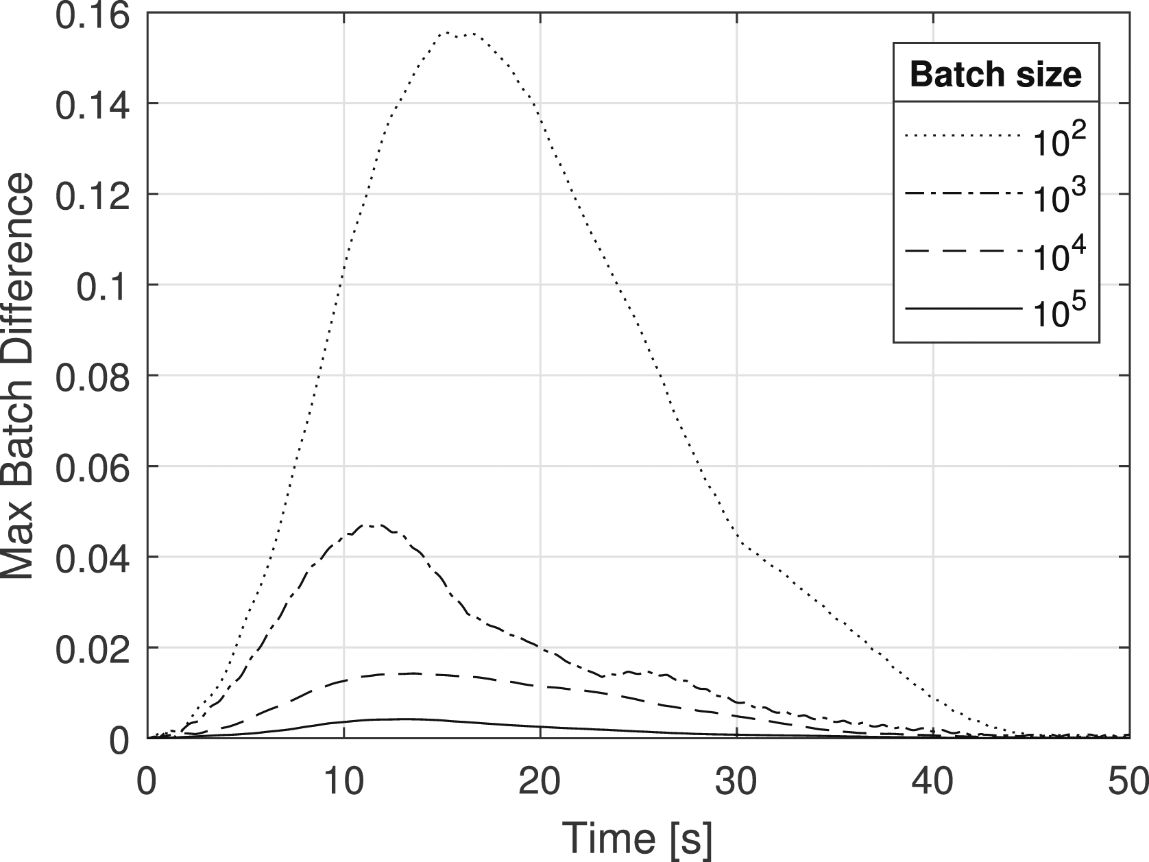
Error characteristics and computation time for varying Monte Carlo simulation batch sizes.
Each MCS produces a system response like that shown in Figure 8. The system response of each MCS is normalised against the initial distance error, which was in turn randomised at the beginning of each simulation. The instantaneous error, ϵ
t
, is given by System response showing different quasi-dynamic guidance law regimes.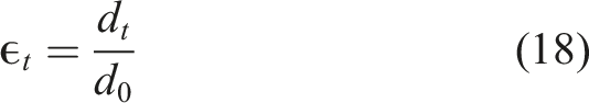
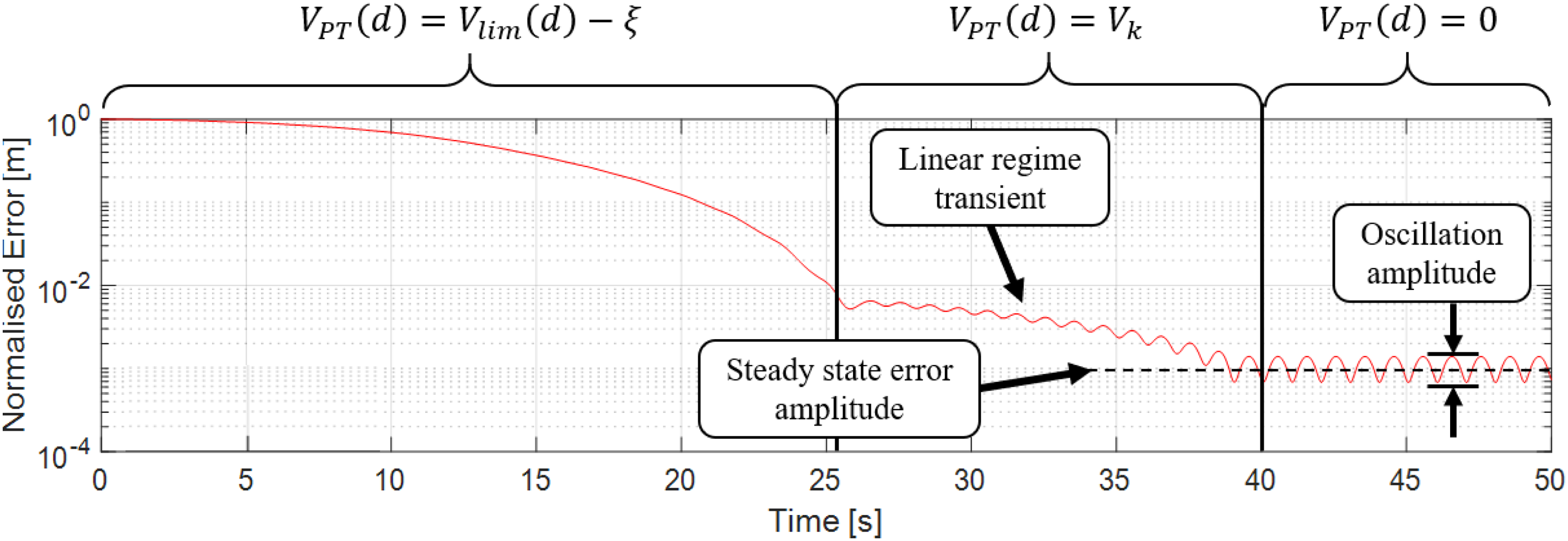
The integral of the normalised system response is thus given by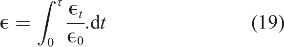
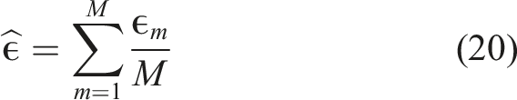
Figure 8 shows an example system response with annotations showing the different regimes governed by equation (17). V PT (d) = V lim (d) − ξ is the closing regime, V PT (d) = V k is the linear regime and V PT (d) = 0 is the stationary regime. In addition, the aspects of the steady state error are the transient, the steady state amplitude and the oscillation amplitude. The transient is also the motion of the projectile in the linear regime; a faster V k provides a faster transient speed. The steady state amplitude can be thought of as the distance d of the ‘orbital centre’ from the target. The oscillation amplitude, and in addition the oscillation frequency, is governed by F c and ω0,1, in which neither can be affected by modifying V k or ξ. These oscillations are caused by the holding orbit described in equation (12); if the locus of the assumed circular orbit coincides with the target, then there will be no oscillations. However, if any small perturbation offsets the orbit loci or the orbit isn’t perfectly circular, the amplitude of the steady state error and steady state oscillations will increase. If the steady state oscillation continues periodically, then the orbit is stable, and the projectile is remaining in the stationary regime. If the steady state has another lower frequency oscillation, the orbit is not stable. This is caused by the linear regime velocity V k being too great for the current d2, causing the projectile to pass straight through the stationary regime. N.B. The regimes are governed by d and so the vertical lines representing them on Figure 8 should be horizontal; this was intentional, to aid interpretation.
Figure 9 illustrates how V
lim
is modified in the QDGL to account for the system response lag. V
lim
acts as the reference signal which the QDGL then modifies using ξ. The closing speed function V
PT
(d) is then passed to the autopilot, which calculates the change in speed per revolution demanded from the projectile’s actuator mechanism V
Dem
. The V
Dem
can then be passed through a chosen controller H, such as a PID. The V
Dem
, modified under the action of controller H, is then passed to the actuator mechanism which saturates the signal such that V
Dem
∈ [0, ΔVmax]. N.B. Vmax is an absolute limit of the system resulting from the maximum bias angle of one half roll revolution, and it is not a characteristic of any physical actuator hardware. If V
Dem
> V
Max
the system will saturate and will only be able to deliver V
Max
. As such, any H > 1 when the autopilot is already demanding V
PT
= Vmax will have no effect on the system whatsoever. Modification of Vlim for speed controller with velocity feedback.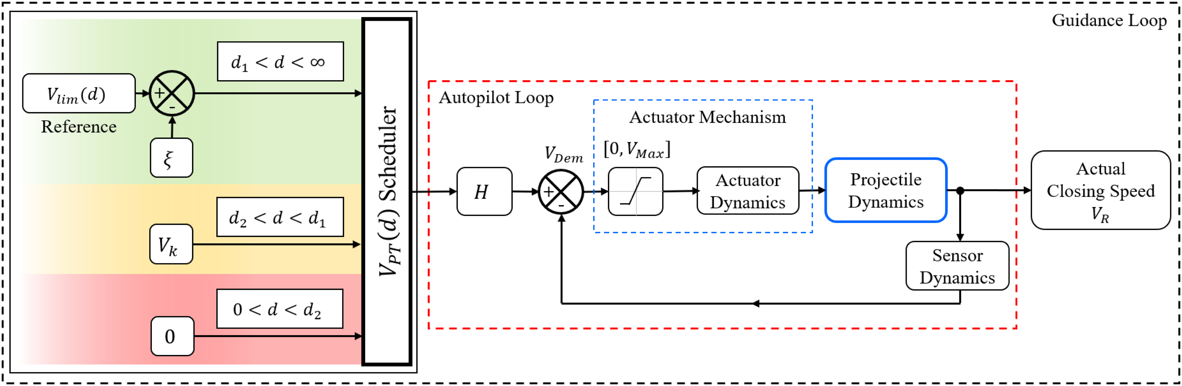
The sensor block shown in Figure 9 represents the sensor dynamics of the system which are assumed in the idyllic system to be perfect and instantaneous. For practical implementation, conventional on-board sensors or an external detection system could be used to measure the roll angle, similar to that described in Ref.18. If volumetric restrictions permit, on-board image sensing hardware could be used. 37 Linear ballistic theory could also be used to estimate the change in roll rate of the projectile along the trajectory beyond what is known from the projectile launch to supplement information from the sensors.
Parametric investigation
With the QDGL fully presented, the system parameters V k , ξ, d1, and d2 can be investigated, with extreme variation in the parameters being shown to demonstrate their functionality and its impact on the system response. A more high-fidelity optimisation is conducted in the Results section. Throughout this section values such as ‘zero’, ‘low’, ‘medium’ and ‘high’ are used when discussing the system response. This is intended to illustrate the change in behavioural differences across the full range of suitable parametric values. However, the exact numeric values are given in the corresponding figure caption.
Figure 10 shows how modifying ξ to extreme values affects the system response. When ξ = 0, the system response exceeds Vlim which was the case in Figure 5 leading to a large overshoot and oscillatory motion where the projectile closes with a speed which is too high. Any negative value of ξ yields a steady state error that is unacceptably high; thus, it is not shown on the figure. For low values, 0 < ξ < 1, the error is reduced quickly with a low amplitude steady state error and no higher order oscillations. High values, ξ ≥ 1, produce a large amplitude steady state error. How extreme values of ξ affect the normalised error (zero: ξ = 0, low: ξ = 0.7, high: ξ = 2).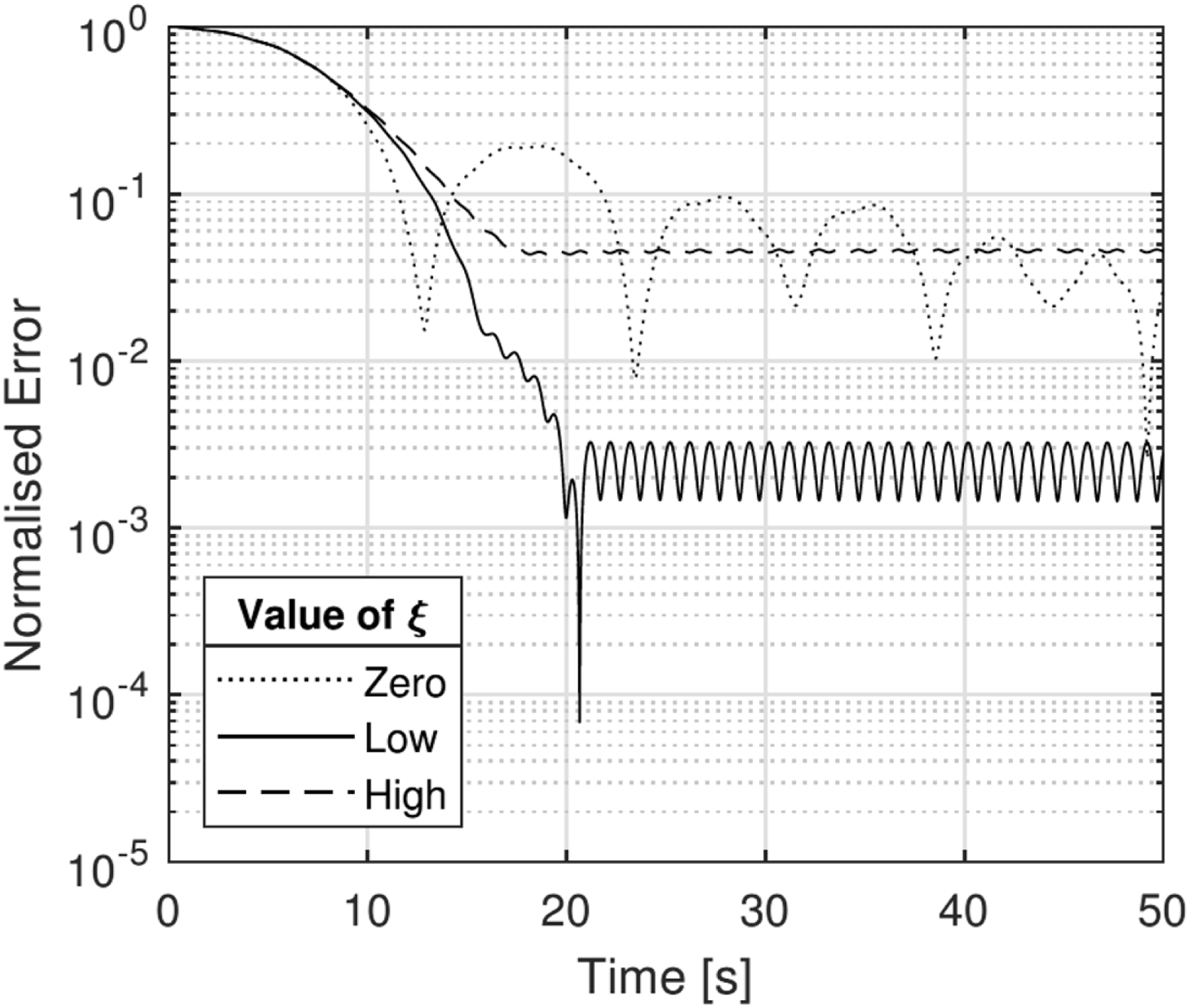
Figure 11 shows three example trajectories which correspond to the extreme values of ξ from Figure 10. The high steady state error for large ξ is represented by the projectile being brought to rest too far from the target. The high amplitude decaying oscillations in the normal error for ξ = 0 is visible as the projectile overshoots the target by a large margin. This is caused by too high a speed being demanded and the projectile is unable to reduce its speed in time due to the system lag. For low values of ξ, the projectile is brought sufficiently close to the target to initiate a regime change. How extreme values of ξ affect the picture plane trajectory (zero: ξ = 0, low: ξ = 0.7, high: ξ = 2).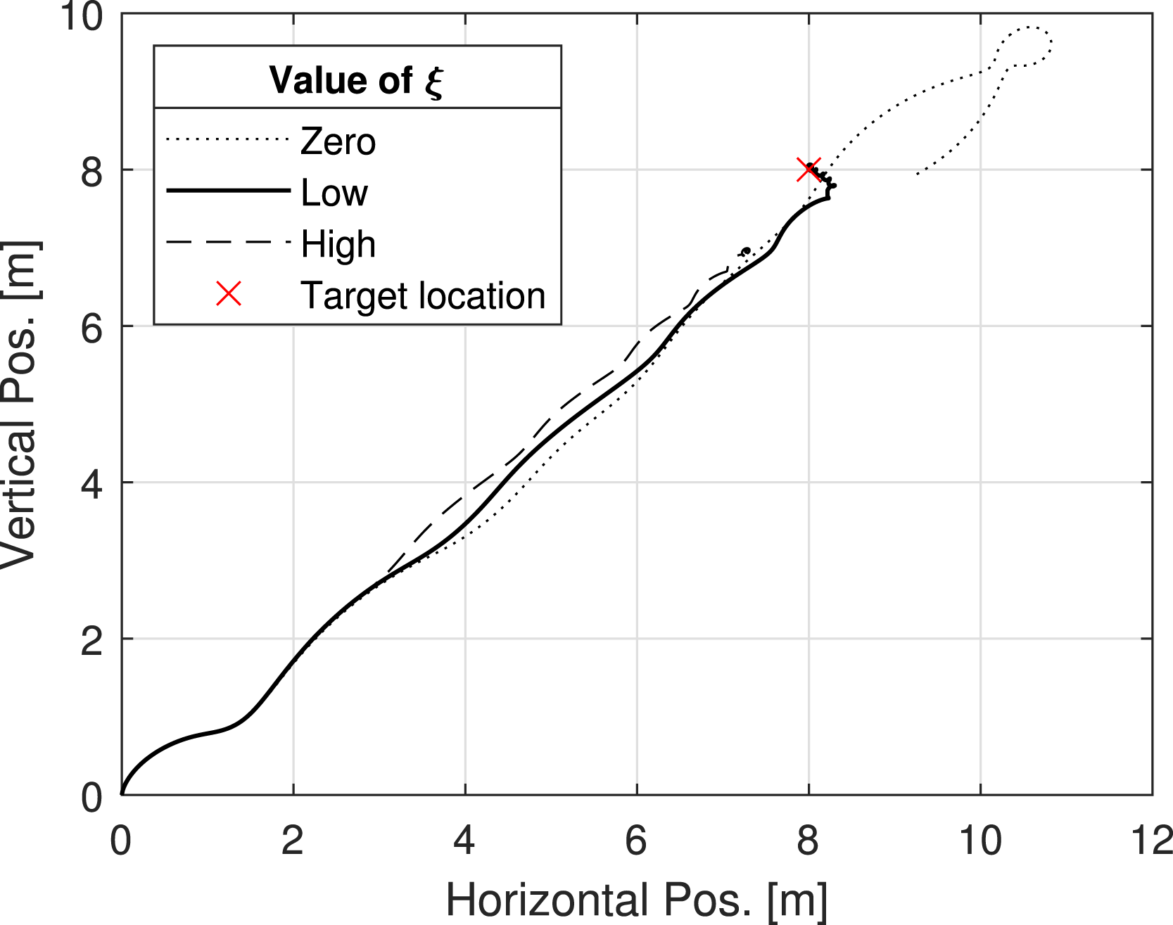
Figure 12 shows the effect of modifying the linear regime constant velocity V
k
. All speeds initially follow the same error reduction path from t = 0 to t = 12. This is the range governed by V
PT
(d) = Vlim(d) − ξ and thus modifying V
k
has no effect. If V
k
is sufficiently small, as the projectile transitions from the linear velocity to the stationary regime, the orbital centre is brought to rest very close to the boundary of the stationary regime, d2. This results in a higher amplitude steady state error than if the velocity was high enough to reduce the distance to d → 0 before it was brought to rest. This is apparent from the figure, as an increasing value of V
k
results in a lower amplitude of the steady state error up to the point that V
k
is too high resulting in an overshoot. The optimal V
k
is a trade-off with d2 to deliver the orbital centre sufficiently close to the target before switching to the stationary regime. How varying V
k
affects the transient and steady state error (zero: V
k
= 0, low: V
k
= 0.01, medium V
k
= 0.2, high: V
k
= 1).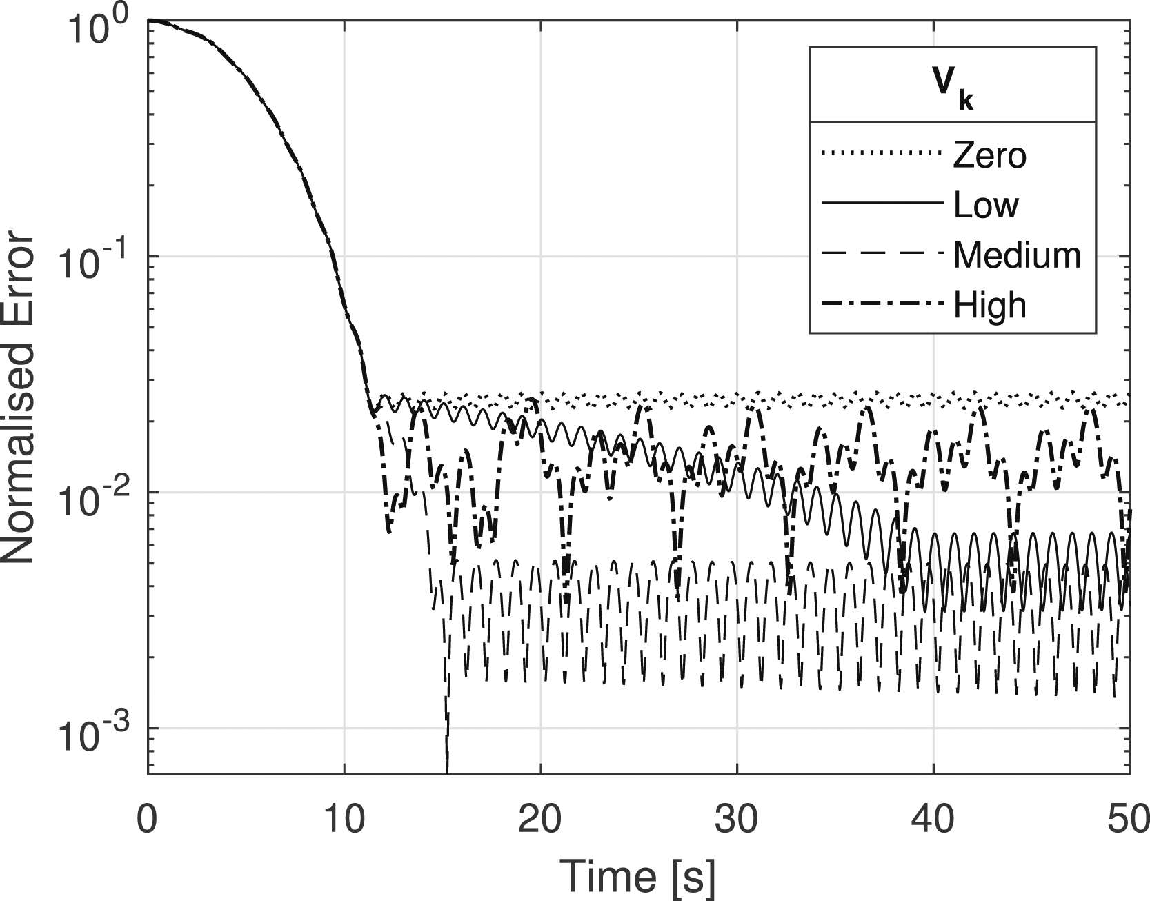
In this case, for V k = 0, the linear regime vanishes, merging with the stationary regime, that is, V PT (d|d ∈ [0, d2]) = V PT (d|d ∈ [d2, d1]) = 0. The result of this is that the projectile enters the stationary regime at a distance d1 and this is apparent from the figure, with a steady but large magnitude steady state error. For low values of V k , the transient is very slow, but the amplitude of the steady state error is small. For medium values of V k , the most desirable system behaviour can be observed. There is a very quick transient period followed by a low steady state error amplitude. For high values of V k , there is an unstable switch between the linear and stationary regimes, caused by a sufficiently high overshoot to exceed d2.
Figure 13 shows the effect of modifying the boundaries of the linear regime, d1 and d1. While d2 is already arbitrary and selected based on the chosen level of accuracy of the system, d1 is calculated from d1| (V
PT
(d1) − ξ = 0) (equation (15)), after a value of ξ has been selected. However, d1 is varied manually here to illustrate the impact of linear regime size. If the boundaries are set to be equal, d1 = d2, then there is ‘no linear regime’, it is bypassed completely and the velocity is brought to relative rest immediately. This leads to a large steady error as was the case for low values of ξ and V
k
. The steady state oscillation amplitude is the same as for any other case, since F
c
, ω0 and ω1 are not being modified. How varying linear regime boundaries affects transient and the steady state error.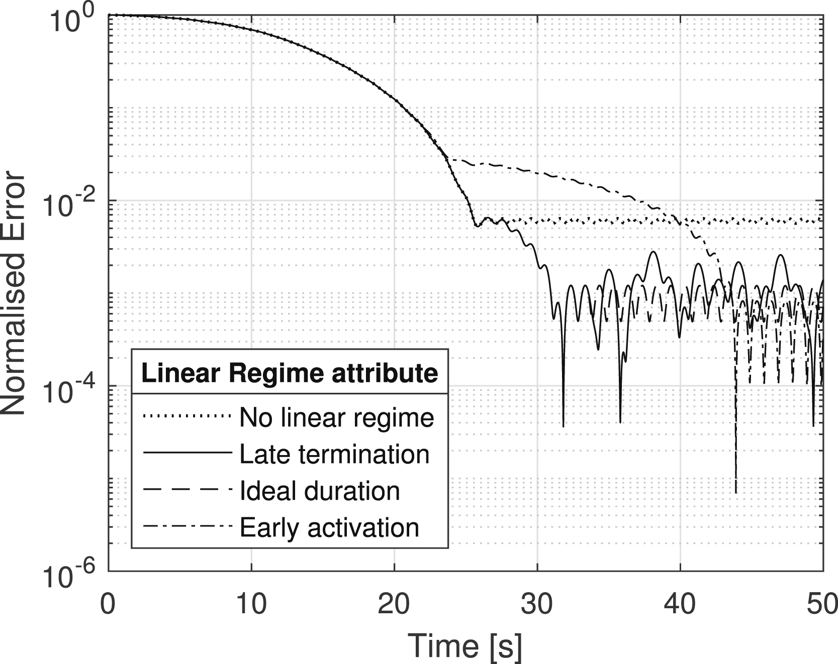
If d2 is small then the projectile gets closer to the target before switching to the stationary regime, this is the ‘Late termination’. When d2 is sufficiently small, it becomes significant compared to the distance that can be travelled by the projectile travelling at speed V k during the time for one complete roll rotation. This results in an unstable steady state oscillation from overshooting, where the projectile continuously switches between the linear and stationary regime, which is indicated by the late regime termination on the figure. In an ‘early activation’, d1 is higher than its true value would be when computed from equation (15). The projectile is brought to the linear regime speed V k too early in time, at a point where Vlim(d) − ξ would have otherwise permitted a higher closing velocity, resulting in a transient period significantly longer than in the other cases. Desirable system behaviour is observed from the ‘ideal duration’ on the figure with a steady transient from the dynamic to the stationary regime followed by a stable steady state oscillation.
The steady state amplitude for early regime activation is lower than the ideal scenario, which is not expected since the lower bound of the linear regime is the same for both simulations. The stationary regime governs all d < d2, which describes a circular area around the target of radius d2. Since the projectile only calculates the bias points when ϕ = 0, the projectile will switch regimes at a different point depending on where the first bias calculation takes place within d2. Small deviations in the trajectory can thus cause a discrepancy in steady state amplitude though the oscillation amplitude will remain the same in all cases. This discrepancy must be mitigated by averaging large number of simulations.
Results and discussion
This section discusses a genetic algorithm used to optimise the QDGL parameters, ξ and V K , as well as the gains of a PID controller. As discussed in the previous section, the values of d1 and d2 cannot be optimised and are therefore not included in this section. The performance of the QDGL with the optimised ξ and V K is then assessed for performance rejection capabilities and evaluated against stationary and moving targets.
System parameter optimisation using genetic algorithm

Range of values for initialisation of Monte Carlo simulation.
The GA converged to the same optimum value for 10 individual trial runs, to within 3sf, and verifying the GA can repeatedly converge to a known optimum solution in the given configuration.
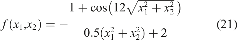
Both the initialisation of the GA and the MCS procedure are stochastic in nature; hence, the optimum value found is not necessarily the ‘true’ optimum. However, the MCS procedure consistently represents the system response to within the desired degree-of-accuracy. In addition, the GA is of low dimensionality and is operating in a relatively low complexity space. This, in conjunction with the consistent performance of the GA when optimising the drop-wave function, reaffirms the optimum values provided by the GA are satisfactory for the scope of this paper.
Using this MCS batch procedure, each specimen of each generation within the GA can now be meaningfully compared such that an optimal solution may evolve. Algorithm 1 shows the order of operations for the GA. The fitness function, FIT, of the GA to be minimised is simply 
The normalised integral error of the system response for the mth MCS follows from equation (19) as
Likewise, the mean normalised integral error of the system response for a Monte Carlo batch of size M for specimen n follows from equation (20) as
The Monte Carlo batch size for the proceeding is M = 104, the justification for which was discussed in the previous section.
Execution of GA optimisation using the MCS procedure 1: Randomly initialise N specimens, 2: 3: 4: Set QDGL parameters equal to specimen 5: Set 6: 7: Run MCS m with random initial conditions 8: Compute ϵ
m
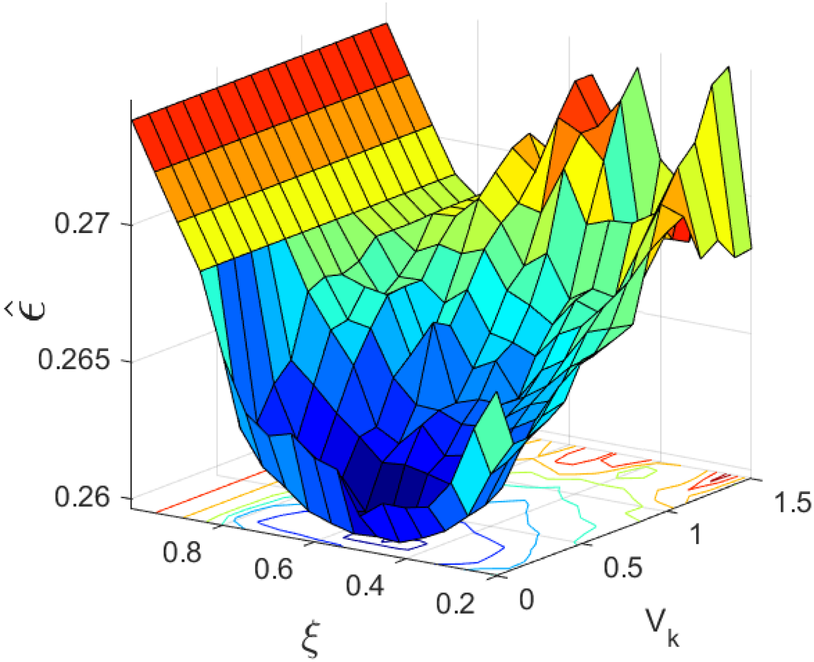
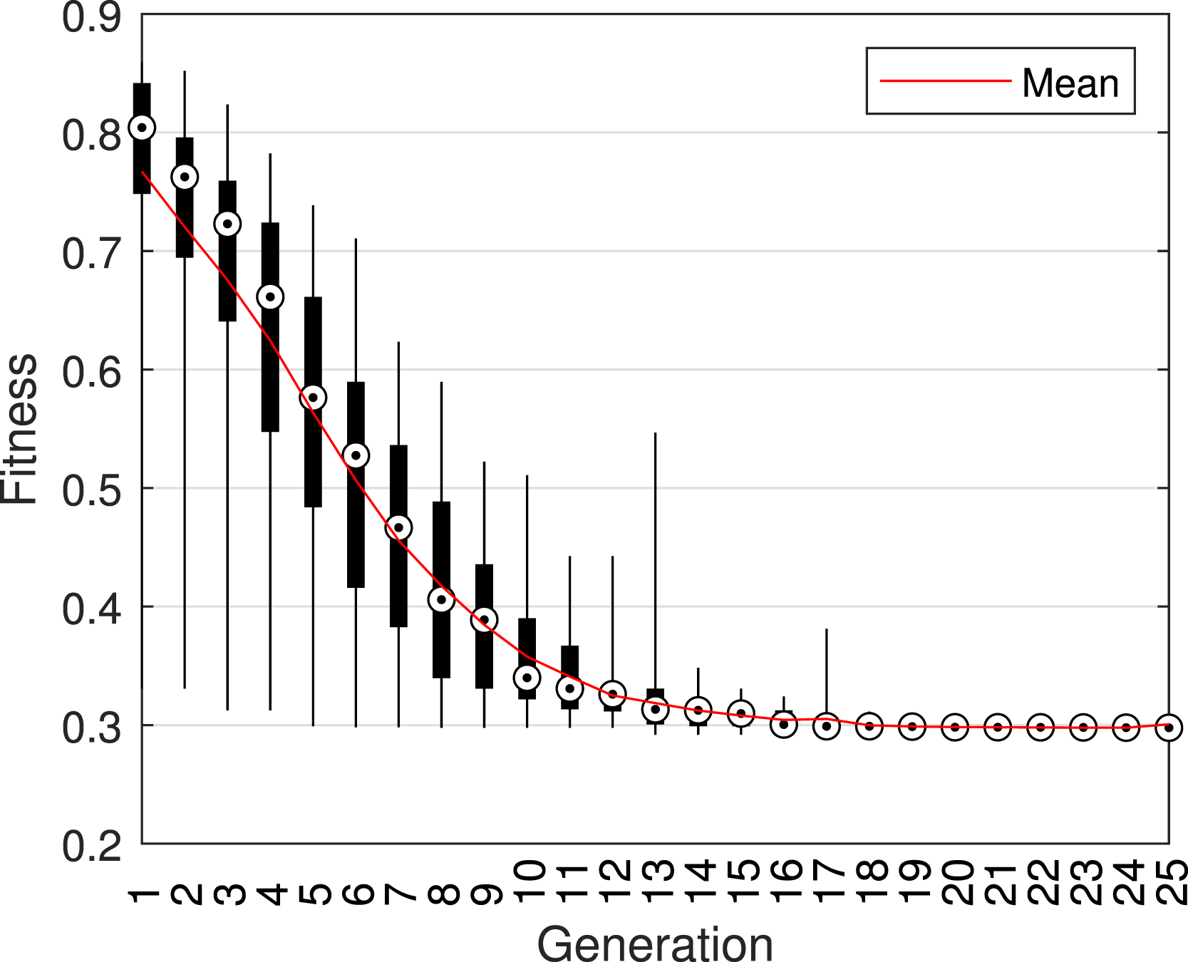
9: end for 10: Compute specimen Fitness: 11: end for 12: Rank specimens in order of fitness and select candidates for reproduction 13: Create offspring from candidates and cull resulting population to size 14: Mutate population, then reduce mutation factor 15: end for To reduce computation time, a preliminary search is conducted to inform the scope of the GA. Figure 14 shows a Figures 15 and 16 show the convergence rate for the GA operating under the boundary conditions for ξ and V
k
. The optimal QDGL parameters from the GA were found to be ξ = 0.54 and V
k
= 0.18.
System response error
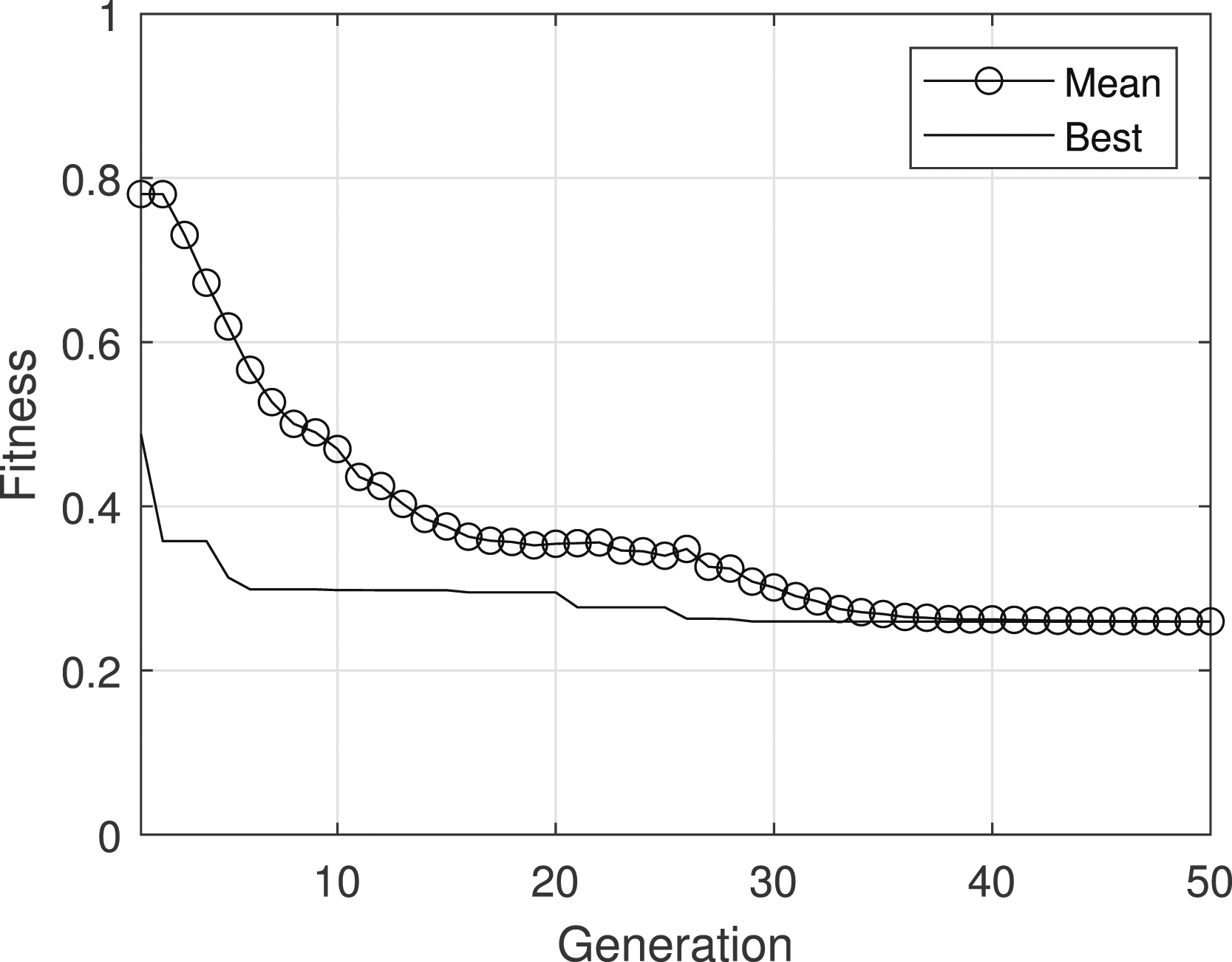
Convergence of 2D GA to optimise quasi-dynamic guidance law parameters.
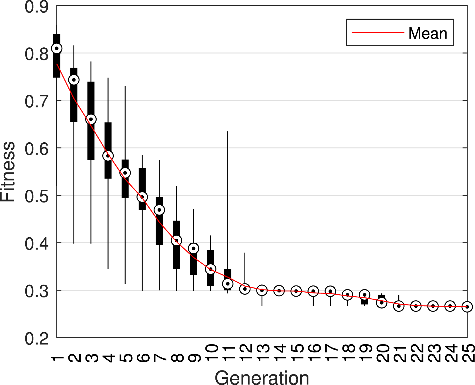
Generation distribution during initial convergence of GA for QDGL parameters.
PID controller gain optimisation
Figure 9 included a block H which represents the chosen controller for V
Dem
. A PID controller is used to investigate the proportional, integral and differential aspects of V
Dem
during feedback. The use may reveal system behaviour that was not otherwise obvious from the previously discussed framework and highlight any weaknesses of the QDGL approach. During the simulation, V
Dem
is decomposed in the YZ plane to the YZ earth axis giving
Figure 17 shows a preliminary search of independently varying the PID controller gains, corollary to Figure 14. The gains are initially held at Contribution of independent k
P
, k
I
and k
D
to the system error.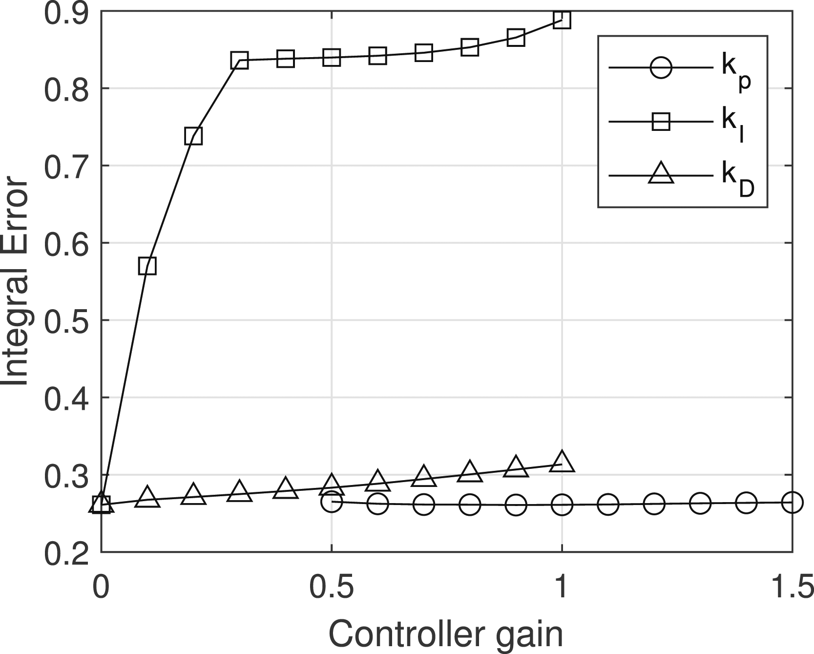
Figures 18 and 19 show the convergence rate of the 3D-adapted GA. The optimal configuration of PID gains was found to be Convergence of 3D GA to optimise PID controller gains. Generation distribution during initial convergence of GA for PID controller gains.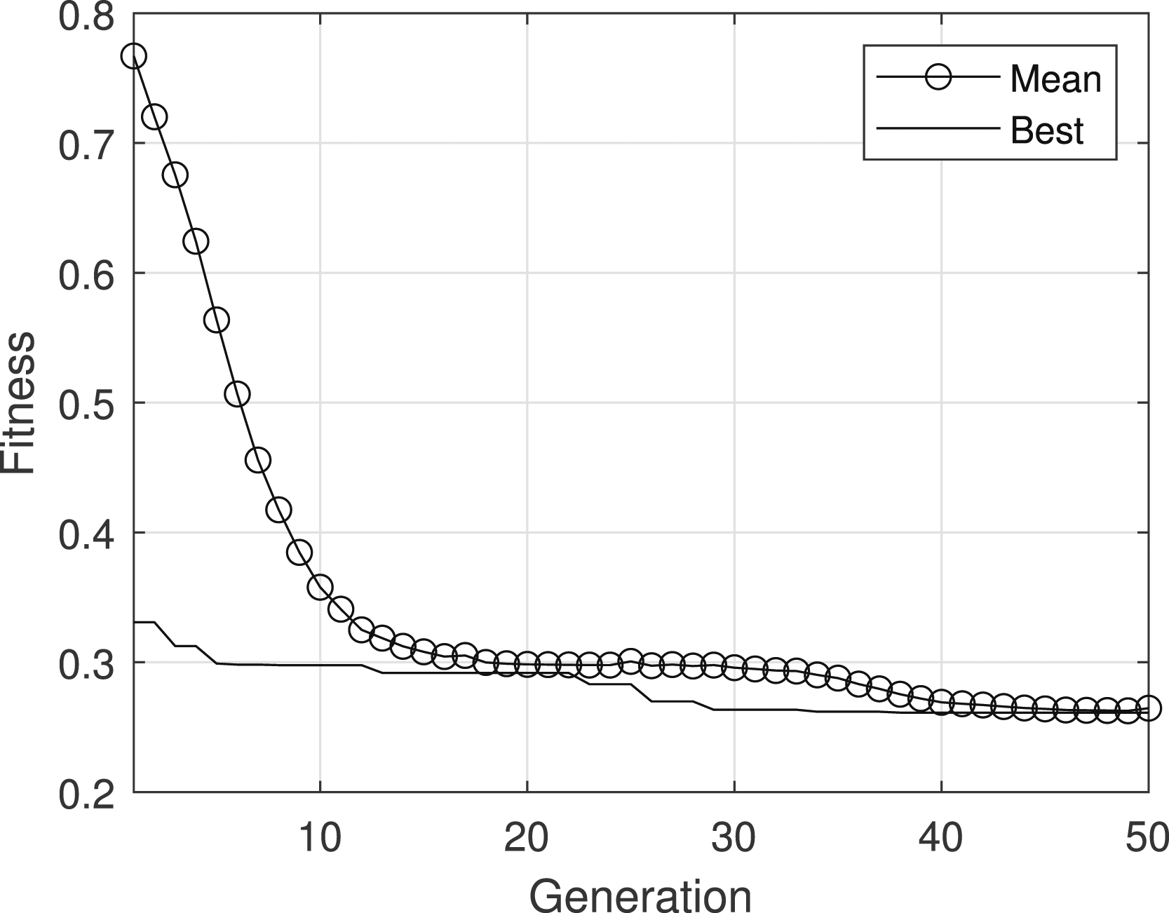
Disturbance rejection and system performance
The optimised QDGL is now tested for disturbance rejection capabilities and performance against different target profiles. Figures 20 and 21 show how the projectile responds to different disturbances. In each case, the projectile and target are initialised at a specified distance, the target closes the distance under normal operation and is then allowed to remain in steady state for a sufficient time until the chosen disturbance is applied and synchronised at 50s. System response to various target distance disturbances. System response to various target velocity disturbances (low: V = 0.01 ms−1, medium V = 0.1 ms−1, high: V = 1 ms−1).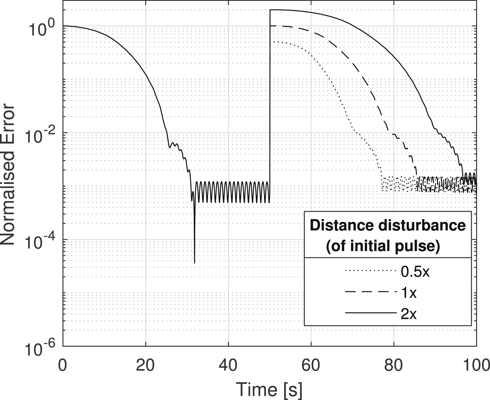
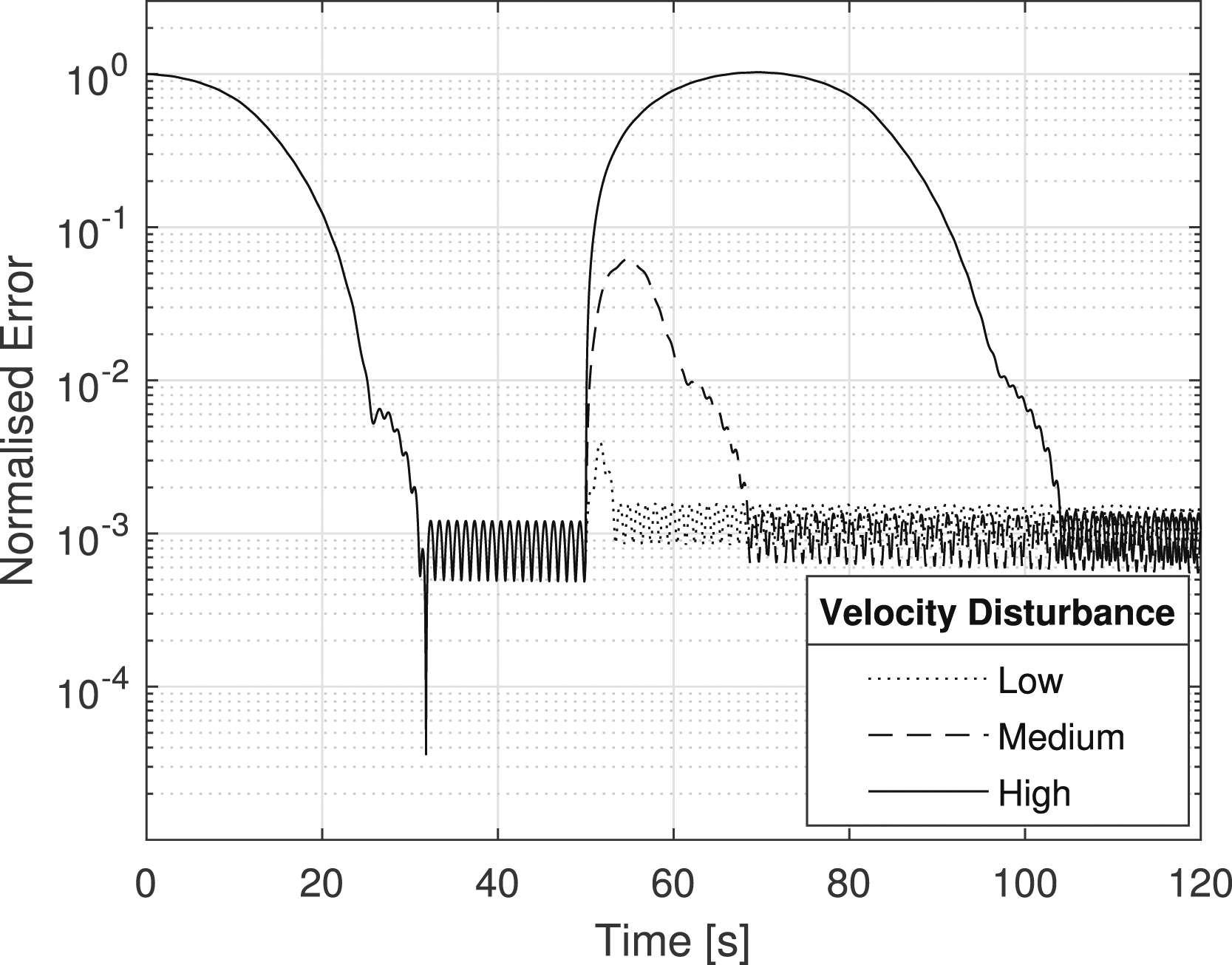
Figure 20 shows disturbance displacements, where at 50s, the target coordinates are set to be at a magnitude of 0.5x, 1x and 2x that of the initial displacement, as indicated by the figure. For all magnitudes of displacement, the error change is discontinuous. The initial correction response is similar for all due to the demand of the velocity autopilot saturating the control mechanism. Once the projectile has slowed sufficiently, it enters the linear regime at the same point in each case, d ≈ 10−2, since the regime switching is governed by a certain distance. There is a small discrepancy between linear regime switching for the disturbances and the initial reference signal. The reference signal enters slightly later at a lower distance. This is likely caused by the projectile crossing the regime threshold d2 with more of the roll rotation left to complete, meaning it will travel longer before the speed is corrected again. The similarity in response is due to the fact that in all cases, the initial relative velocity between the projectile and target is zero, and thus, the system will respond as if the simulation has just been initialised at different distances.
Figure 21 shows velocity displacements, where at 50s, the relative velocity of the target is instantaneously changed to a low, medium and high respective speed, radially away from the projectile. The positions of the projectile and target are not changed; they are then free to dynamically evolve. When the velocity disturbance is low, within what the actuator mechanism is capable of correcting in one roll rotation, the disturbance is corrected quickly. With a medium disturbance, beyond the correction of one bias manoeuvre, the system takes longer to recover. Since this is a velocity disturbance, the maximum error increase is not instantaneous, rather it coincides with the instant where the target is no longer moving away from the projectile and the relative speed is zero. From this point, the closing of the projectile is similar to the distance disturbances. This is the same for the high velocity disturbance, except that the rate of reduction of error divergence takes longer to correct.
Figure 22 shows the average normalised error for a 104 MCS batch against both stationary and moving targets. The response against stationary targets is the same as previously in this section. Against moving targets, however, the error initially increases a small amount before decreasing in a manner similar to the response against static targets. This initial increase is due to the random chance of the projectile being initialised with speeds directed away from the target, and then having to correct this dispersive motion before beginning the correction procedure. Performance of the quasi-dynamic guidance law against target profiles.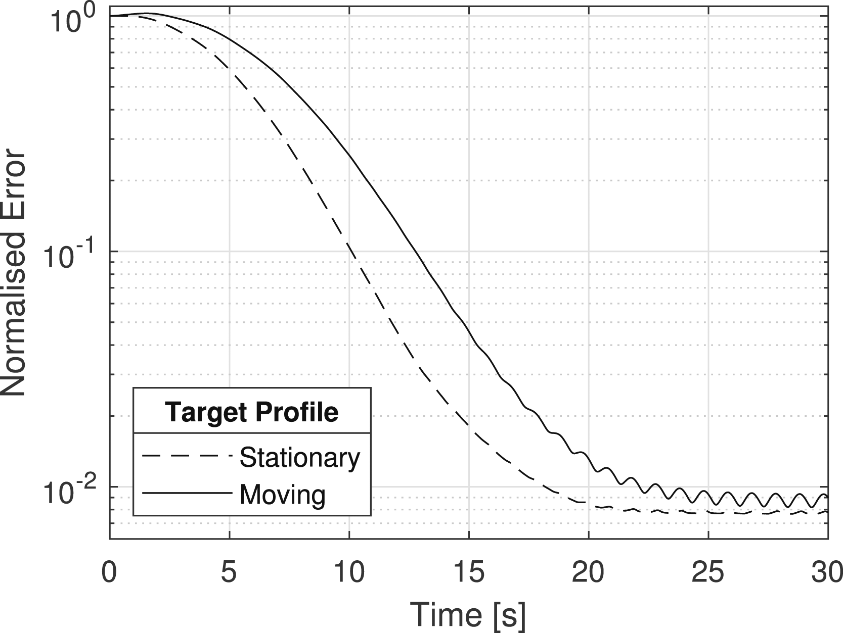
Conclusions
A 7 DOF dynamic model for a dual-spin projectile (DSP) is presented and implemented in computational simulations. A novel projectile design is presented along with the unconventional control method of asymmetric roll-rate biases. The quasi-dynamic guidance law (QDGL) is developed and a parametric study is conducted which shows how modifying QDGL parameters affect the system response. A Monte Carlo simulation (MCS) procedure is described, which is used to meaningfully compare the system response for different parameter configurations. A genetic algorithm which utilises the MCS procedure is then used to optimise the QDGL parameters and PID controller gains. The disturbance rejection capabilities of the optimised QDGL are tested, as well as the effectiveness against both static and dynamic targets. In all cases, the QDGL is able to reduce the distance error to a satisfactory level.
Full dynamic coupling and aerodynamic disturbances have not been considered in this paper but will be the topic of further investigations. In addition, the use of this QDGL should be explored with a dynamic or time dependant control force and arbitrarily complex roll rate switching profiles.
Footnotes
Declaration of conflicting interests
The author(s) declared no potential conflicts of interest with respect to the research, authorship, and/or publication of this article.
Funding
The author(s) disclosed receipt of the following financial support for the research, authorship, and/or publication of this article: This paper was sponsored by EPSRC ICASE Grant reference 1700 064 and BAE Systems
Data availability
The data that support the findings of this study are available from the corresponding author, James N., upon reasonable request.