Sage Journals: Discover world-class research

Abstract

A technique has been developed to analyse the free-space acoustic signature of the Rolls-Royce Merlin engine in order to provide diagnostic information relating to its performance. The work is motivated by a need to maintain the reliability and maximise the lifetime of this historic engine which is an important component of the aircraft operated by the UK Battle of Britain Memorial Flight (BBMF). For convenience, the data were extracted from the soundtrack of a video recording made whilst the aircraft was undergoing a full-power ground-run. The aim of the work is to generate information relating the individual firings of each cylinder and this is presented as a multi-level colour image. Here, the ignition time history for two revolutions (six ignitions) is shown vertically and corresponds to the bank of exhaust ports facing the microphone. Subsequent similar histories are presented along the horizontal time axis. The results are sensitive to engine speed variations, and a correlation between successive vertical columns is carried out to quantify this drift and adjust the data accordingly. Seven engine speeds from 842 to 2740 rpm are examined. The processed data illustrate that some speeds exhibit well-defined, single ignitions whereas others show varying degrees of after-firing type effects. At the higher engine speeds, it would seem that the cylinder ignition amplitudes become much more irregular, and the results for 2740 rpm indicate a breakdown in engine performance. The coefficient of variation (Cv) has been demonstrated as a measure of these factors. Finally, a technique has been proposed and demonstrated for the identification of individual cylinders in the firing sequence. The data acquisition process is relatively straight-forward and should not demand excessive time to cover a full range of engine speeds. With further investigations, it could be possible to readily relate the imaging results to specific engine faults.

Keywords

Acoustic signature Battle of Britain Memorial Flight combustion engine diagnostics Merlin ignition

Introduction

Monitoring techniques play a major role in assessing the performance of aircraft engines. Over the years, many different methods have been adopted and the majority have required making physical contact between the engine and the sensor. This could be via a connection to a traditional cockpit instrument,^1–3 or by applying temporarily a specialised device for research purposes,⁴ possibly under laboratory conditions. An alternative approach is to acquire engine performance information by remote access, where the sensor is a significant distance away. This can be attractive in that it can be applied easily to different aircraft having the same engine type and avoids the need for the fitting of special sensors. In this case, the information of interest is carried by the acoustic wave radiating from the engine or airframe, and it can be recorded by employing one or more suitable microphones. Such acoustic data are often recorded digitally and lend themselves to further sophisticated data processing to retrieve the required performance parameters.

Remote acoustic measuring techniques have been proposed for a variety of aerospace applications. Perhaps the earliest example was the use of concrete reflectors, between about 1916 and the 1930s, to provide early warning of incoming enemy aeroplanes and airships,^5,6 but these had limited range. More recently, in situations where range is less important, acoustic investigations have been carried out to classify aircraft type, or measure location and speed.^7–9 A passive acoustic system has been examined for the covert detection, tracking and classification of low flying aircraft crossing an international border.¹⁰ Estimates of aircraft speed, heading, frequency spectrum and altitude are made and aircraft are classified as helicopter, piston engined, turboprop or jet. Other work using passive acoustic sensors employs the Doppler effect through a genetic algorithm, to locate the position of manoeuvring aircraft.¹¹ The rise in popularity of multi-rotor unmanned aircraft systems has stimulated research into their nuisance contribution in urban environments, close to humans and dwellings. Ref. 12 reports work carried out on a quad-rotor aircraft, employing sound pressure level meter measurements in the field and sound source localisation using an acoustic array in a laboratory environment. Further work on unmanned aerial vehicle (UAV) tracking and localisation is reported in Refs. 13–15, and an examination of the multiple-UAV localisation problem in a dynamic contested environment is described in Ref. 16.

Noise mapping of sound sources around airports is used to assess the environmental impact of overflying aircraft. Developments of this, applied to aircraft on approach, have used spectral analysis to provide more sophisticated results to characterise dominant frequency components and relate them to their likely origins on the airframe and the engine.¹⁷ In recent years, airframe components such as flaps, slats and landing gear have become increasingly significant contributors to overall aircraft noise, and the phased microphone array^18,19 has provided a means of identifying these features. A suitable inversion process is required to estimate the location and strength of these separate contributions and²⁰ provides an extensive review of the imaging algorithms widely used in aeroacoustic experiments, ranging from the simple conventional beamforming technique to the more computationally intensive deconvolution and inversion methods.

The phased microphone array is extensively employed in wind tunnels, which offer a controlled environment for the investigation of scaled models^21–23 or aircraft components,^24–26 although exact replication of flight conditions is difficult due to factors such as modelling accuracy, high background noise level and discrepancy in the Reynolds number.

Other acoustic engine measurements at ground level include the possibility of pre-flight fault detection²⁷ and the visualisation of full-scale jet noise for tied-down tactical aircraft such as the F-22A Raptor.^28–30 Work on spectral decomposition of engine noise is described in Refs. 31 and 32, and the identification of noise sources from aeroengine fans by using phased arrays has been reported.^33,34 Acoustic measurements have also been proposed as a means of deducing engine power settings during start-up and take-off, which are often not published by the airlines. As a measure of thrust, the rotational speed of the low-pressure shaft is deduced by extracting its corresponding radiated frequency component, through generation of a spectrogram using the short-time Fourier transform.³⁵

Inevitably, the most reliable results for engine and airframe noise emissions are obtained for full-size aircraft in operational conditions, although these bring problems of propagation effects and moving sources.^36–39 Again, the phased microphone array provides a valuable insight into the aeroacoustic mechanisms and enables the identification and analysis of the distribution of noise sources on the aircraft.^40–44 Furthermore, the microphone array is proving of value in measuring the noise variability arising from the wide range of conditions associated with aircraft of different types when taking off or landing.^45–48

This article examines a new microphone measurement technique which is appropriate to various types of internal combustion engine, but here is applied in particular to the Rolls-Royce Merlin engine. The Merlin engine is essential to ensure the continuing operation of the historic Spitfire, Hurricane and Lancaster aircraft which form part of the UK Battle of Britain Memorial Flight (BBMF). In order to ensure that the BBMF can pursue its national role, it is important to maintain the reliability of this engine and maximise its lifetime. Accordingly, it is worth examining possible engine diagnostic techniques which might support this need. Such solutions should be easy to implement and readily cover the full range of operating speeds. Furthermore, they would be attractive if they could be used with low-cost instrumentation and require no modification to the existing ground-run test procedure.

In 2016, a video was posted on YouTube to illustrate a full-power ground-run of BBMF Spitfire MK356.⁴⁹ According to the description, the aircraft had sustained an engine unserviceability and had to be ground-run to establish the cause of the fault. After studying this video, it was decided to examine the soundtrack, in order to establish whether useful diagnostic information could be obtained from the acoustic record. Figure 1 shows a screenshot from the video which indicates the location of the camera during the test. This article describes the procedures involved.

Figure 1.

Screenshot from video.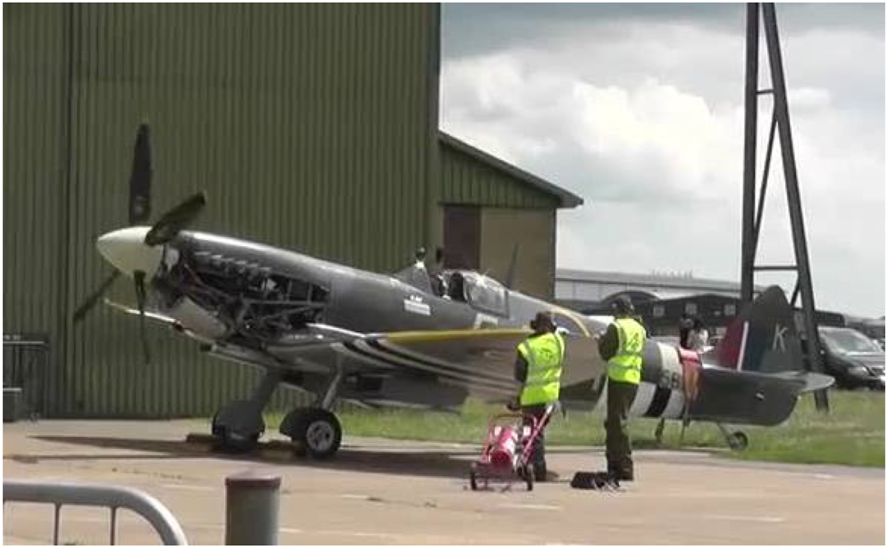

Features of the acoustic record produced

The Merlin engine operates through a sequential firing of its individual cylinders, each ideally producing a well-defined pulse of exhaust emission which generates a sound impulse. A typical cylinder will fire once every two revolutions of the engine and it is the sum of the responses from all cylinders which will be sensed by a human observer or a microphone. This signal has the characteristics of a pulse train with a particular mark-space ratio, or duty cycle, and will give rise to a corresponding frequency spectrum, which will be discussed later. It is important to note that for the measurements discussed here, only half of this pulse train is available, and this corresponds to the bank of exhaust ports facing the microphone. From the data, it is evident that the other bank, facing away from the microphone, does not generate a significant acoustic amplitude at the microphone. For a complete firing record, a second microphone would be located symmetrically to the first microphone, at the other side of the aircraft.

Measurement parameters

It is important to be able to relate engine speed to the various frequencies present in the sound spectrum produced by the exhaust emissions.

Let the engine speed be N rpm, or (N/60) revolutions per second, so that the time for one revolution is 60/N s. Two revolutions of the Merlin engine are required for 12 cylinder firings and the time for this is

T_{12} = \frac{2 \times 60}{N} s

(1)

This is also the time for six cylinder firings along one bank,

T_{6}

, and so the time between individual firings on one side of the engine,

T_{F}

, is given by

T_{F} = \frac{T_{6}}{6} = \frac{20}{N} s

(2)

The frequency (or first harmonic) associated with these firings,

F_{F}

, is given by

F_{F} = \frac{1}{T_{F}} = \frac{N}{20} Hz

(3)

The range of engine speeds and corresponding first harmonic parameters for the Merlin engine is, typically, from 1000 (50 Hz) to 3000 rpm (150 Hz).

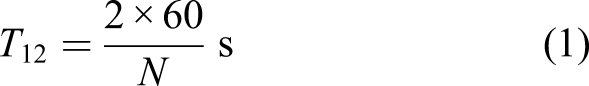
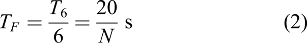
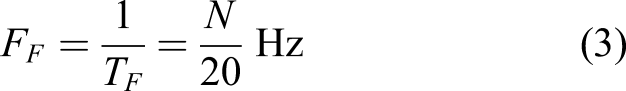
If the first harmonic $F_{F}$ of the frequency spectrum is known, then the engine speed can be found from equation (3) so that $N = 20 F_{F} rpm$ . The pulse train produced by the acoustic signal from the engine has a frequency spectrum composed of an infinite number of harmonics which are multiples of the fundamental. As will be shown later, it is beneficial to view how this frequency spectrum varies with time.

Data processing

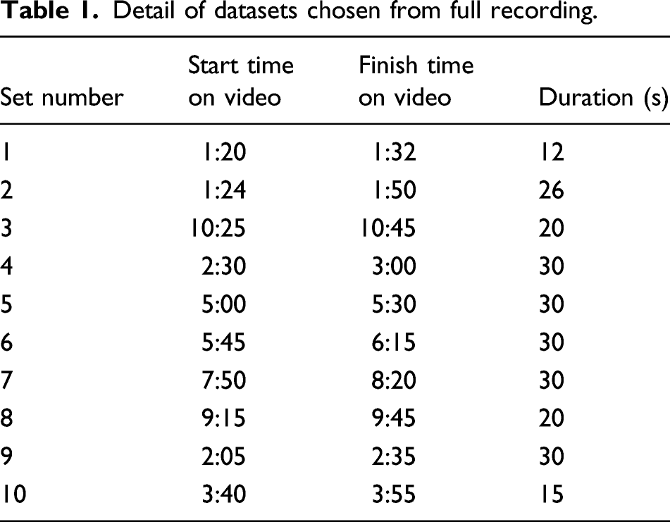
The first stage of processing involved conversion of the audio soundtrack of the video into a WAV file. This was carried out using the Standard Edition of Total Recorder⁵⁰ set to a stereo sampling rate of 48 kHz. These data were then converted into ASCII format by using a routine written in GNU Octave.⁵¹ In all, 10 sets of data were chosen from the full recording to represent a range of different engine operating conditions. These are summarised in Table 1. The majority of the subsequent processing was carried out using software written in Fortran.⁵²

Table 1.

Detail of datasets chosen from full recording.

Set number	Start time on video	Finish time on video	Duration (s)
1	1:20	1:32	12
2	1:24	1:50	26
3	10:25	10:45	20
4	2:30	3:00	30
5	5:00	5:30	30
6	5:45	6:15	30
7	7:50	8:20	30
8	9:15	9:45	20
9	2:05	2:35	30
10	3:40	3:55	15

Short-time Fourier transform processing

In dealing with acoustic data where the frequency response is likely to vary with time, it is very informative to employ the short time-Fourier transform (STFT) to generate a spectrogram. In this way, particular features can be easily identified and extracted for further processing.

As an example, the STFT of Set 5 is shown in Figure 2, over a 40 dB dynamic range. (The ‘jet’ rainbow colourmap has been chosen to enhance the visualisation of the results presented in this article. Should the images be reproduced in a monochromatic format, the features of interest will still be preserved). The video demonstrates a substantial increase in engine speed at around 5:06 and this is seen in the STFT as a significant increase in the frequencies of the spectral components. At 5:10, the engine speed is gradually reduced and this is also clear in the STFT as all spectral components return to their earlier values. It should also be noted that the image shows clearly the cut-off effect of the microphone at frequencies approaching zero.

Figure 2.

STFT of Set 5.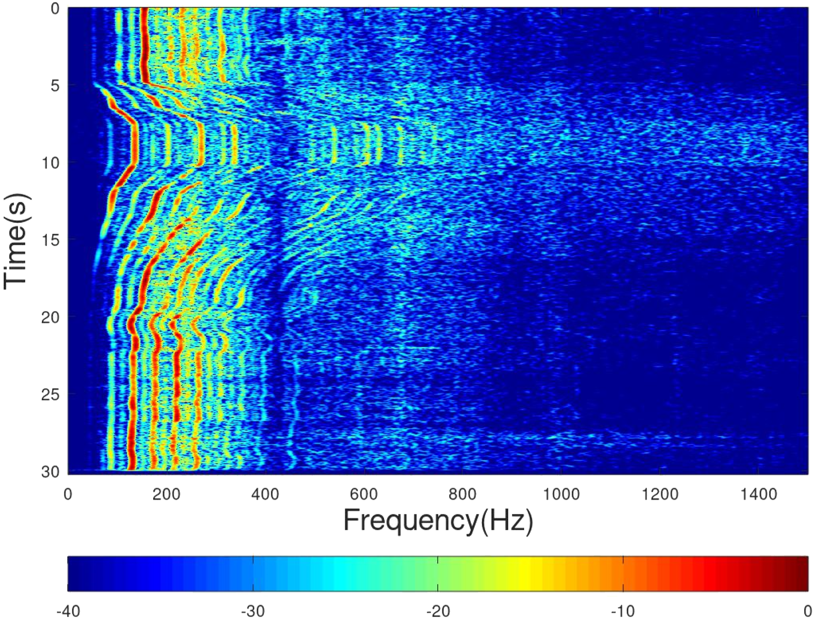

As mentioned later, an accurate measurement of the fundamental frequency must be deduced from the STFT, and for this reason, the raw data are interpolated by a factor of 16 in the frequency domain.

General procedure

The sequential firing of the cylinders generates a regular sequence of pulses in the time domain, and the aim of this work is to generate information on the individual firings of each cylinder. In order to achieve this, suitable processing of the time-domain data is needed. In particular, it was necessary to make significant corrections for the frequency response of the microphone used on the video camera. For typical engine tick-over speeds, the STFT results show that frequencies as low as 50 Hz are produced and these are outside the normal audio bandwidth of the microphone. By examining the low-frequency roll-off shown in the STFT, a correction function of approximately 18 dB per octave was derived and used as the first step in the data processing. Whilst this has been sufficient for demonstrating the feasibility of the procedure, microphones with good low-frequency responses should be used for more rigorous applications of the technique.

After carrying out frequency response correction of the raw data, it is beneficial to improve the signal to noise ratio and this was carried out in software by using a moving average filter⁵³ to reduce unwanted higher frequency components. This filter is optimal in that it produces the lowest noise for a given edge sharpness, which is attractive for pulse information retrieval. The filter width was arrived at by examining its effects on the data set where the ignition sequences are very well-defined. It was found that inter-pulse noise contributions increased as the filter width was reduced below one-third of the acoustic pulse width and so this was chosen as a lower limit. To satisfy this requirement for the range of acoustic pulse widths under consideration, a moving average filter width of 2.3 ms was used.

Inevitably, the zero-frequency, or dc level, of the pulse train is lost in the recording process, and the recorded data consist of the fundamental frequency and higher order harmonics. In defining the pulse edges, the zero crossover of this waveform is a sensible choice because it relates to an optimum threshold in terms of the original PAM waveform. To aid interpretation of the results, data below the threshold are set to zero.

Figure 3(a) shows a typical time-domain response obtained from the recorded acoustic waveform of Set 4, from approximately 2:57 to 3:00 in video time.

Figure 3.

(a) Time domain response and (b) pulse period extracted for Set 4.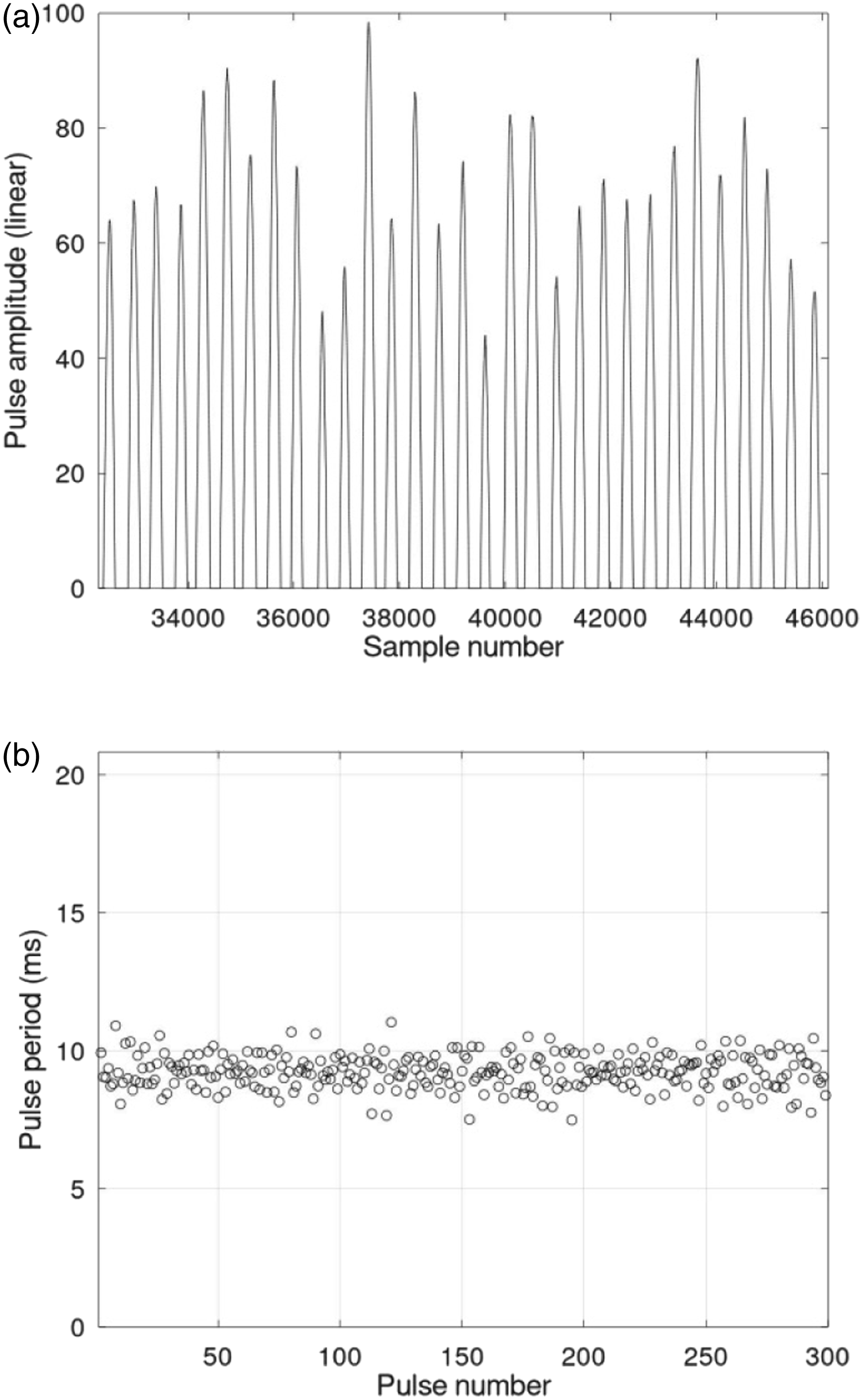

13,814 samples are presented on the horizontal time axis and these correspond to a time window of approximately 0.288 s. Amplitude variations are seen and these will be a measure of differing cylinder output levels. The finite slope on the rising and falling edges is due to the rise time of the ignition process and also the use of the moving average filter. The filter does not, however, significantly affect the zero crossover positions or the peak values, and so the integrity of these important parameters is maintained.

Using a software edge detection procedure, the number of samples between successive pulses can be found and is shown in Figure 3(b) for a longer section of the waveform, of duration 2.8 s. The mean value of this response is 446 samples, which corresponds to a pulse period of 9.29 ms and an engine speed of 2152 rpm.

Ignition data are presented as a multi-level colour image with the ignition time history for two revolutions (six ignitions) shown vertically and with subsequent similar histories presented along a horizontal time axis. The time associated with the vertical axis length is 6/ $F_{F}$ where $F_{F}$ is the fundamental frequency associated with the engine speed. If the engine speed changes, then engine ignitions will not occur at the same vertical time and the response will drift either upwards or downwards as time goes by. The value of $F_{F}$ is deduced by careful measurement of the fundamental frequency from the STFT for the time interval under consideration. Sequential blocks of data corresponding to time intervals of 6/ $F_{F}$ are then extracted and used to build the image.

As an example of this, consider the ignition data for Set 3 from 10:30 to 10:40, which is shown in Figure 4(a) over a linear amplitude range. The sequence for the six ports is seen clearly, but it is evident that the engine speed is varying over the time interval. For exactly constant engine speed, six horizontal responses would be expected.

Figure 4.

Ignition history for Set 3 from 10:30 to 10:40, (a) without and (b) with correlation adjustment.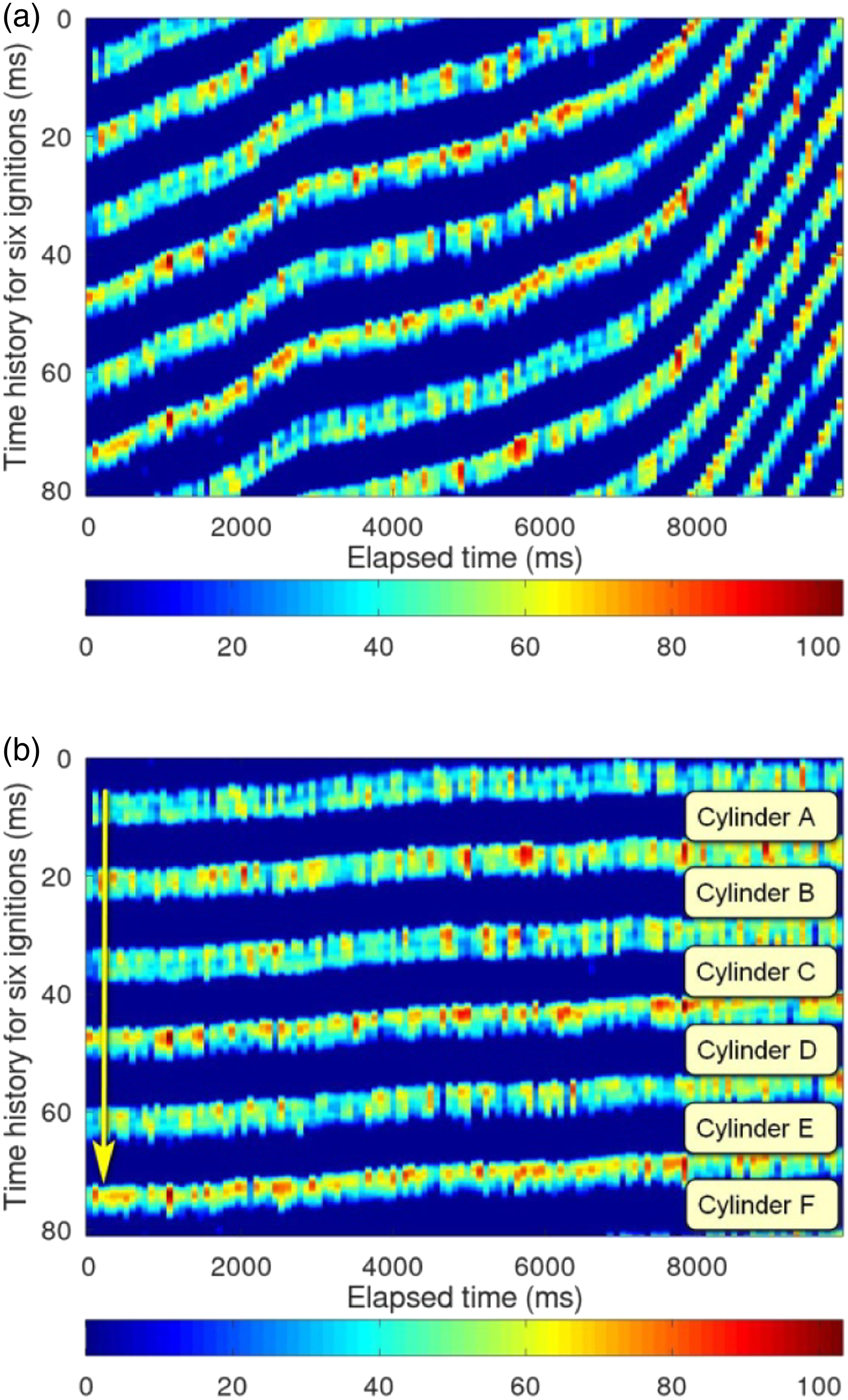

To correct for this, a correlation between successive columns is carried out to quantify the drift and adjust the data accordingly. Note that the correlation output is a speed variation monitor. Following this procedure, the image becomes that shown in Figure 4(b).

Whilst not perfect, the procedure has removed the majority of the speed variation problem and enables a much clearer interpretation of the data. In this result, a very clear and well-defined ignition sequence is seen, with quiet zones between successive ignitions. The arrow indicates the sequence of ignitions (cylinders A to F) for each engine cycle. For each cylinder, approximately 124 successive ignitions have been mapped over the 10 s period. There is evidence of differences in performance between cylinders, and procedures are available to extract the power output variations for each individual cylinder as time goes by.

It should be noted that these sequential ignitions are generated by a non-sequential cylinder firing order and care must be taken in relating the above results to particular cylinders. This raises an interesting challenge as to how the performance of a particular cylinder can be identified and a suggestion of how this might be achieved is discussed later. Despite this limitation, the technique can still provide useful information on engine performance.

Results of data analysis

In an attempt to cover a reasonably representative engine speed range, the acoustic datasets shown in Table 2 were extracted from the soundtrack. The data lengths are limited at the higher engine speeds, but still provide useful results. In any future investigations, a more complete set of engine speeds could be specified. Note that the speeds shown above are average values over the range of the data record.

Table 2.

Datasets chosen for representative speed range.

Nominal engine speed (rpm)	Set duration (seconds)	Video time interval
842	10	05:55–06:05
990	5	02:30–02:35
1037	10	09:25–09:35
1482	10	10:30–10:40
1659	2.1	02:37.3–02:39.4
2173	2.8	02:56.9–02:59.7
2740	11	03:44.6–03:51.2

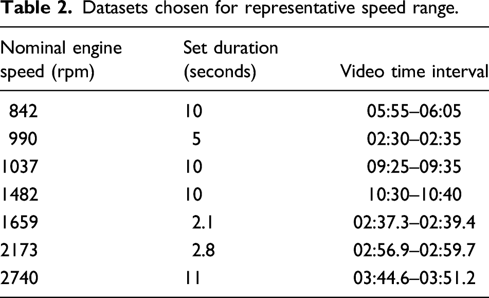
The processed data show a range of interesting results, illustrating that some speeds exhibit well-defined, single ignitions whereas others show varying degrees of after-firing type effects. At the higher engine speeds, it would seem that the cylinder ignition amplitudes become much more irregular, and the results for 2740 rpm indicate a breakdown in engine performance. These results are discussed in more detail below.

Considering Figure 5(a), the video indicates that engine hunting is taking place during this period. Careful examination of the ignition record indicates that there are six regularly spaced dominant firing sequences, one for each cylinder. Each of these is followed shortly by a weaker firing sequence and then a further, less-weak sequence. The pattern is regular for all cylinders.

Figure 5.

Ignition histories.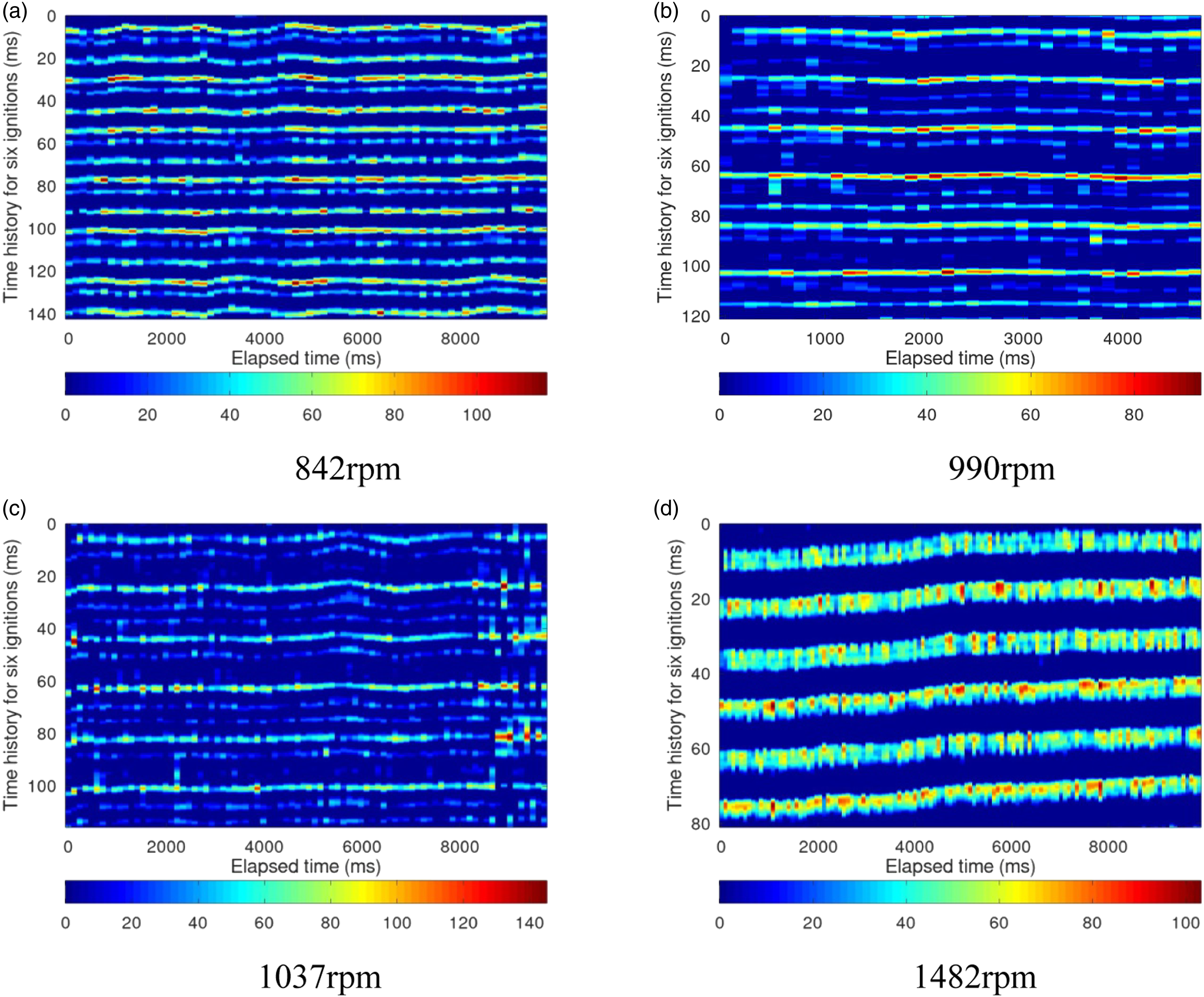

Following the increase in engine speed to 990 rpm, Figure 5(b) shows that the six regularly spaced dominant firing sequences are now much more obvious, as a result of reduced after-firing. It is interesting to note the existence of several smeared-out after-firing bursts.

After a further small increase in engine speed to 1037 rpm, once again there are six regularly spaced dominant firing sequences, as seen in Figure 5(c). Following the labelling convention introduced in Figure 4(b), primary ignitions A, C and E appear to be followed by single after-fires, whereas primary ignitions B, D and F exhibit double after-fires.

The result in Figure 5(d), for 1482 rpm, appears to show a significant improvement in engine performance, with six very well-defined ignition sequences, and no visible after-firing effects. There are, however, noticeable variations in output amplitude for each cylinder as time progresses. By tracking each response, this change can be extracted and displayed. The following results relate to the peak amplitude, but it is also possible to extract information proportional to the average power in each ignition pulse. The peak amplitude variations for each cylinder are shown in Figure 6(a) on a linear scale.

Figure 6.

(a) Peak amplitudes for each cylinder at 1482 rpm; (b) positions of amplitude peaks at 1482 rpm.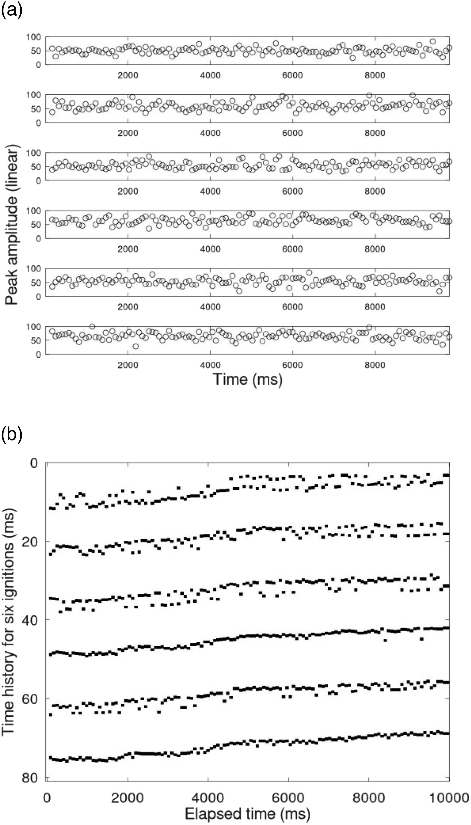

A different presentation can be used to enhance the visibility of the peak amplitude positions, which are shown by the horizontal dark lines in Figure 6(b). These marker lines indicate the consistency of ignition onset from one pulse to the next. It is seen that sequences D and F show good consistency, whereas the remaining sequences are more erratic and demonstrate regular deviations in the timing of ignition onset. Here, the deviation is of the order of 2.5 ms (equivalent to around 22° crank angle change at this speed) and is likely to have a noticeable effect on engine performance.

Increasing the speed from 1482 to 1659 rpm initiates a further onset of after-firing effects. As shown in Figure 7(a), sequences B, D and F exhibit obvious smeared-out after-firing bursts.

Figure 7.

Ignition histories and STFT.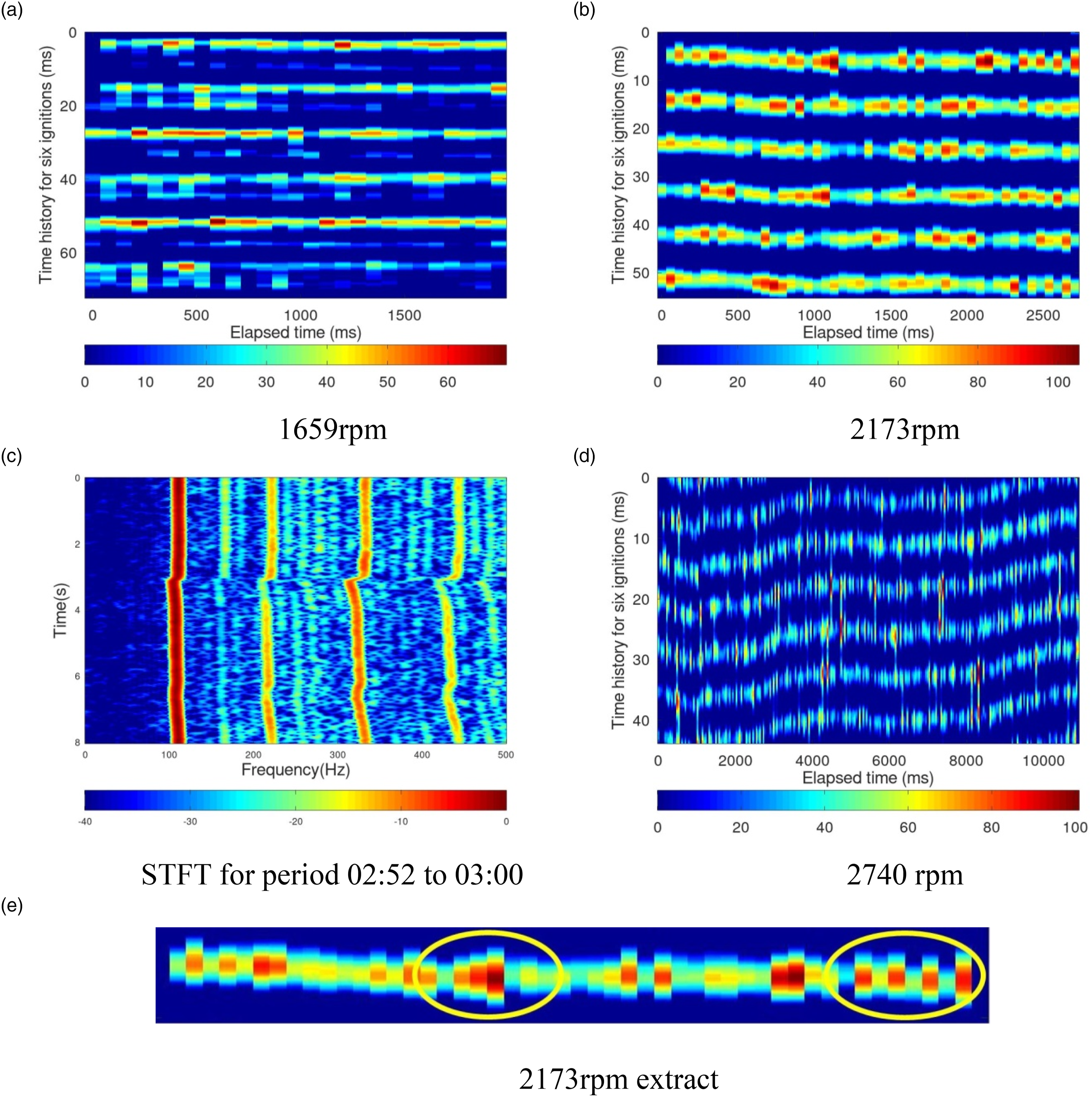

After a further increase in speed to 2173 rpm, Figure 7(b) indicates a return to six very well-defined ignition sequences and no visible after-firing effects. However, it is clear that for all cylinders the output power varies considerably as time progresses. Certain interesting features are seen in the top ignition sequence which is shown again in Figure 7(e). In the left-hand highlighted selection, a gradual build-up of output power occurs over four successive ignitions, and then this is immediately followed by a set of low-power outputs. In the right-hand highlighted selection, successive alternations between high- and low-power outputs are seen.

It is interesting to view the STFT just prior to and during the time period associated with Figure 7(b), and this is shown in Figure 7(c). What appears to be a sudden loss in power is evidenced by the discontinuity seen at a time of 3 s (02:55 on the soundtrack), where the engine speed falls rapidly by around 110 rpm. Over the next 5 s, the engine gradually recovers its original speed. No clear evidence of power loss is seen from the ignition histories for this period, but in the current investigation, these do not include information from the other bank of cylinders. It is worth noting the sensitivity of the STFT to this type of fault and that it may offer a useful signature for utilisation in automatic feature recognition software.

In Figure 7(d), where the engine is operating near to its maximum speed, performance has been degraded, and the firing sequences are very erratic, with significant variations in power output as time evolves.

Cv as a measure of engine performance

The coefficient of variation (Cv) is a statistical measure of the dispersion of data points in a data series around the mean. It represents the ratio of the standard deviation to the mean and in this work it is proposed that it can be used to examine irregularities in the firing sequence. Irregular firing sequences for a cylinder imply more stress on the engine, leading to more wear and reduced life. It is therefore argued that Cv might be a quantitative measure of these effects.

Figure 8 shows the resulting values of Cv obtained from the peak amplitudes at seven different engine speeds over the range considered. Consistent values of Cv are seen from 842 rpm up to 2173 rpm, but the result for 2740 rpm returns a much higher value. This latter result implies an increased firing irregularity, and this is evident when the sets of firing images are studied in Figures 5 and 7.

Figure 8.

Cv results.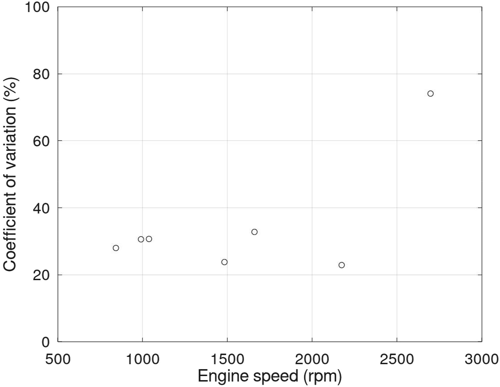

Identification of individual cylinders in firing sequence

It would be beneficial to be able to relate a particular ignition sequence to the cylinder which produced it, but the single microphone measurement method described here does not permit this. A technique is now proposed that overcomes this restriction by employing the measurement configuration shown in Figure 9,⁵⁴ where two separate microphones are used to record the acoustic signal from the engine. For convenience, the broadside direction of this two-element array is directed towards the centre of the exhaust stack, but this is not critical to the method. The cylinders are assumed to be numbered as 1 to 6 from the propeller end of the engine towards the rear of the aircraft.

Figure 9.

Measurement configuration using two-element microphone array. (Microphone locations not to scale and are typically 20 m distant from the engine).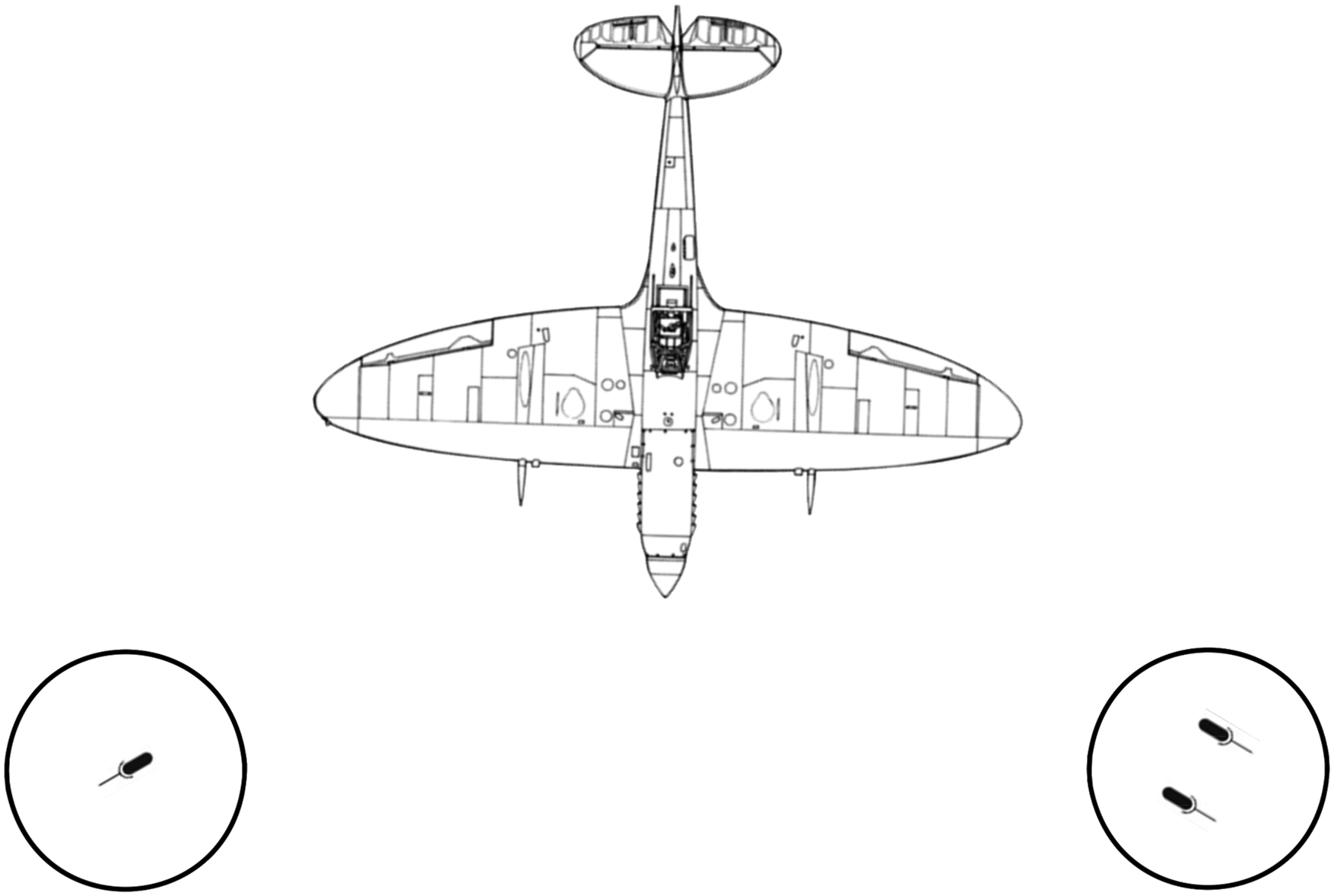

Consider the difference signal derived from the two microphone channels. In this case, the arrangement can be viewed as a two-element receive array with a null in the broadside direction. By applying a suitable time shift between the channels, this null can be steered away from broadside in either direction. Clearly, we now have the ability to point the null at a particular exhaust port and cancel the acoustic signal received from it. Consequently, the multi-level colour image of the ignition time history will clearly indicate the missing signal and so enable identification of the cylinder involved. The width of this null is not zero and hence it will introduce some attenuation of the difference signal from adjacent cylinders. Despite this, a clear indication of the correct cylinder is still obtained.

Uncertainty in knowing the direction of the synthesised null is not a problem. In practice, it is straightforward to choose a time shift which positions the null direction well away from the exhaust stack. At this stage, the multi-level colour image of the ignition time history will show strong signals for all six cylinders. Now, by gradually adjusting the time shift to steer the null towards and across the port stack, observation of the corresponding ignition time history will indicate a sequential disappearance and re-appearance of image rows which will enable identification of corresponding cylinders. It is recognised that calibration of the two microphone channels will be advisable to normalise their outputs.

In order to demonstrate this technique, as far as possible with real signals, the results used earlier for the nominal engine speed of 2173 rpm have been adapted. For convenience, it has been assumed that the first data pulse corresponds to Port 6 in Figure 9 and that the firing sequence is cylinders 6, 5, 4, 3, 2 and 1. It is recognised that this differs from the true sequence, but it should offer an easier understanding of the results to be presented below. By extracting individual data pulses from the time sequence, the time-domain signals that would be received at the two microphones can be synthesised.

These data can now be processed with appropriate time shifts. Consider cases where the null is steered to point at each port location in sequence from 6 to 1. Figure 10 shows the corresponding ignition time histories, over a 30 dB dynamic range, where the top ignition image row corresponds to cylinder 6 and the bottom row to cylinder 1. It is clear that the cylinders can be correctly related to their ignition sequence. It can be seen that the nature of the image rows has changed due to the difference algorithm applied, the central nulls being derived from taking the difference between two slightly shifted pulses. It should be noted that this method only requires the measurement of signals from one bank of six ports because of the known relative firing sequence for the complete set of 12 ports. Indeed, the correct relationship need only be extracted for one port to allow the remainder to be deduced.

Figure 10.

Ignition time histories resulting from null being steered to point at each port location in sequence from Port 6 to Port 1.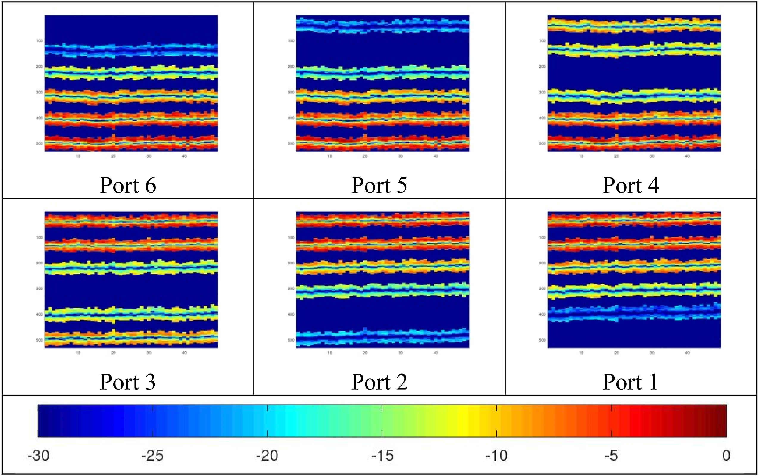

Conclusions

A technique has been developed to analyse the free-space acoustic signature of the Merlin engine and provide diagnostic information relating to its performance. It has been shown that individual cylinder ignitions can be identified and data extracted relating to their power output and firing pattern.

A correlation process has been successfully applied to compensate for engine speed variations and reduce the drift in the ignition histories displayed.

Some simplifications have been made to the data processing. An approximate correction function was used to compensate for the microphone frequency response. Confidence in this was confirmed elsewhere by comparing its effects with theoretically generated frequency response data. However, in future tests, this limitation would be removed by using microphones with good low-frequency responses. An additional simplification was to use a fixed width for the moving average filter at all engine speeds, despite differences occurring in the acoustic pulse widths at the exhaust ports. Investigations showed that this gave improved noise performance and did not markedly affect the zero crossover positions or the peak values so maintaining the integrity of these important parameters. Finally, the engine speeds are specified as average values over the duration of any data record, but in future tests, more precise control of speed would remove this limitation.

The processed data show a range of interesting results, illustrating that some speeds exhibit well-defined, single ignitions whereas others show varying degrees of after-firing type effects. At the higher engine speeds, it would seem that the cylinder ignition amplitudes become much more irregular, and at the highest measured speed of 2740 rpm, there would appear to be a breakdown in engine performance. The Cv has been demonstrated as a measure of these factors.

Further investigations would be of value in demonstrating the capabilities of this technique. It is proposed that two microphones having good low-frequency responses would be used to capture information relating to all 12 cylinders. An additional third microphone would be employed if cylinder identification were to be needed. Furthermore, it is recommended that a well-defined range of engine speeds be examined to provide a more comprehensive analysis of engine performance.

A technique has been proposed and demonstrated for the identification of individual cylinders in the firing sequence. The method utilises a pair of microphones receiving signals from one bank of cylinders and is tolerant of positioning errors.

The data acquisition process is relatively straight-forward and should not demand excessive time to cover a full range of engine speeds. With further investigations, it could be possible to readily relate the imaging results to specific engine faults and provide a means of optimising the performance and lifetime of the engine.

Work is also being carried out to examine the feasibility of applying this process to an aircraft in the flypast mode.

Footnotes

Declaration of conflicting interests

The author(s) declared no potential conflicts of interest with respect to the research, authorship, and/or publication of this article.

Funding

The author(s) received no financial support for the research, authorship, and/or publication of this article.

ORCID iD

John C Bennett

References

Federal Aviation Administration . Flight instruments. Pilot’s Handbook of Aeronautical Knowledge. www.faa.gov/regulations_policies/handbooks_manuals/aviation/phak/.

Schroer

. Cockpit instruments [A century of powered flight:1903-2003]. IEEE Aerosp Electron Syst Mag 2003; 18(7): 13–18.

Chorley

. Seventy years of flight instruments and displays. Aeronaut J 1976; 80(788): 323–342.

Ilic

Rasuo

Jovanovic

, et al. Impact of irregularities in the piston engine operation on the inflight vibration level. In: 29th Congress of the International Council of the Aeronautical Sciences. St Petersburg, Russia, 7 September 2014, pp. 4749–4754.

Scarth

. Echoes from the sky: Acoustic detection of aircraft. Chicago, IL: Independent Books, 2017.

Sockett

EWA

. Concrete listening mirror at Fulwell, Sunderland. Durham Archaeol J 1990; 6: 75–76.

Tong

Xie

Y-H

, et al. Estimation of low-altitude moving target trajectory using single acoustic array. J Acoust Soc America 2016; 139(4): 1848–1858.

Sendt

Pulford

Gao

, et al. A system for automatic classification of aircraft flyovers using acoustic data. In: Final Program and Abstracts on Information, Decision and Control, Adelaide, SA, 11–13 February 2002, pp. 169–174.

Ferguson

Quinn

. Application of the short‐time Fourier transform and the Wigner-Ville distribution to the acoustic localization of aircraft. J Acoust Soc America 1994; 96(2): 821–827.

10.

Nielsen

. Acoustic detection of low flying aircraft. In: IEEE Conference on Technologies for Homeland Security. Boston, MA, 2009, pp. 101–106. doi: 10.1109/THS.2009.5168021.

11.

Martin

Genesca

Romeu

, et al. Passive acoustic method for aircraft states estimation based on the Doppler effect. IEEE Trans Aerospace Electron Syst 2014; 50(2): 1330–1335.

12.

Kloet

Watkins

Clothier

. Acoustic signature measurement of small multi-rotor unmanned aircraft systems. Int J Micro Air Vehicles 2017; 9(1): 3–14.

13.

Blanchard

Thomas

J-H

Raoof

. Acoustic localization and tracking of a multi-rotor unmanned aerial vehicle using an array with few microphones. J Acoust Soc America 2020; 148(3): 1456–1467.

14.

Guo

Ahmad

Chang

. Classification, positioning, and tracking of drones by HMM using acoustic circular microphone array beamforming. EURASIP J Wireless Commun Networking 2020; 1(2020): 1–19.

15.

Ferguson

Gao

, et al. Aircraft flight parameter estimation using acoustic multipath delays. IEEE Trans Aerosp Electron Syst 2003; 39(1): 259–268.

16.

Manickam

Swar

Casbeer

, et al. Multi-unmanned aerial vehicle multi acoustic source localization. Proc Inst Mech Eng G: J Aerosp Eng 2021; 235(3): 273–294.

17.

Khardi

. An experimental analysis of frequency emission and noise diagnosis of commercial aircraft on approach. J Acoust Emission 2008; 26: 290–310.

18.

Billingsley

Kinns

. The acoustic telescope. J Sound Vibration 1976; 48(4): 485–510.

19.

Billingsley

. A comparison of the source location techniques of the acoustic telescope and polar correlation. J Sound Vibration 1978; 61(3): 419–425.

20.

Merino-Martínez

Sijtsma

Snellen

, et al. A review of acoustic imaging methods using phased microphone arrays. CEAS Aeronaut J 2019; 10(1): 197–230.

21.

Oerlemans

Broersma

Sijtsma

. Quantification of airframe noise using microphone arrays in open and closed wind tunnels. Int J Aeroacoustics 2007; 6(4): 309–333.

22.

Blacodon

. Analysis of the airframe noise of an A320/A321 with a parametric method. J Aircraft 2007; 44(1): 26–34.

23.

Guo

Joshi

Noise characteristics of aircraft high lift systems. AIAA J 2003; 41(7): 1247–1256.

24.

Ramos do Amaral

Himeno

FHT

do Carmo Pagani

, et al. Slat noise from an MD30P30N airfoil at extreme angles of attack. AIAA J 2018; 56(3): 964–978.

25.

Bulté

Redonnet

. Landing gear noise identification using phased array with experimental and computational data. AIAA J 2017; 55(11): 3839–3850.

26.

Guo

Yamamoto

Stoker

. Experimental study on aircraft landing gear noise. J Aircraft 2006; 43(2): 306–317.

27.

Miljkovic

Fault detection for aircraft piston engine by exhaust noise analysis. In: Proceedings of the 34th International Convention MIPRO, Opatija, Croatia, 23–27 May 2011, pp. 756–761.

28.

Wall

Gee

Gardner

, et al. Near‐field Acoustical holography applied to high‐performance jet aircraft noise. Proc Mtgs Acoust 2011; 9(1): 040009.

29.

Wall

Gee

Neilsen

, et al. Cylindrical acoustical holography applied to full-scale jet noise. J Acoust Soc America 2014; 136(3): 1120–1128.

30.

Harker

Gee

Neilsen

, et al. Source characterization of full-scale tactical jet noise from phased-array measurements. J Acoust Soc America 2019; 146(1): 665–680.

31.

Miles

. Separating turbofan engine noise sources using auto- and cross spectra from four microphones. AIAA J 2008; 46(1): 61–74.

32.

Neilsen

Vaughn

Gee

, et al. Three-way spectral decompositions of high-performance military aircraft noise. AIAA J 2019; 57(8): 3467–3479.

33.

Caldas

Greco

Pagani

, et al. Acoustic imaging of in-duct aeroengine noise sources using rotating beamforming and phased arrays. IEEE Trans Comput Imaging 2017; 3(3): 485–492.

34.

Shah

White

Hensley

, et al. Continuous-scan phased array measurement methods for turbofan engine acoustic testing. J Eng Gas Turbines Power 2019; 141: 081201.

35.

Schluter

Becker

. Determination of aircraft engine speed based on acoustic measurements. Hamburg, Germany: Inter-Noise, 2016, pp. 778–785.

36.

Howell

Bradley

McCormick

, et al. De-Dopplerization and acoustic imaging of aircraft flyover noise measurements. J Sound Vibration 1986; 105(1): 151–167.

37.

Camier

Padois

Provencher

, et al. Fly-over source localization on civil aircraft. In: 19th AIAA/CEAS Aeroacoustics Conference, Berlin, Germany, 27–29 May 2013, pp. 2013–2261.

38.

Ruijgrok

. Elements of aviation acoustics. 2nd ed. Delft, The Netherlands: VSSD, 2007.

39.

Sijtsma

. Beamforming on moving sources. National Aerospace Laboratory (NLR). Tech. Rep. NLRTP-2006-733, 2006.

40.

Piet

Michel

Böhning

. Localization of the acoustic sources of the A340 with a large phased microphone array during flight tests. In: 8th AIAA/CEAS Aeroacoustics Conference, Breckenridge, CO, 2002, pp. 2002–2506.

41.

Guérin

Siller

. A hybrid time-frequency approach for the noise localization analysis of aircraft fly-overs. In: 14th AIAA/CEAS Aeroacoustics Conference (29th AIAA Aeroacoustics Conference), Vancouver, BC, 5–7 May 2008, pp. 2008–2955.

42.

Merino-Martínez

Snellen

Simons

. Functional beamforming applied to imaging of flyover noise on landing aircraft. J Aircraft 2016; 53(6): 1830–1843.

43.

Fleury

Malbéqui

. Slat noise assessment from Airbus A340 flyover phased-array microphone measurements. AIAA J 2013; 51(7): 1667–1674.

44.

Khorrami

Lockard

Humphries

, et al. Preliminary analysis of acoustic measurements from the NASA-Gulfstream airframe noise flight test. https://ntrs.nasa.gov/citations/20080018649.

45.

Simons

Snellen

van Midden

, et al. Assessment of noise level variations of aircraft flyovers using acoustic arrays. J Aircraft 2015; 52(5): 1625–1633.

46.

Vieira

Snellen

Simons

. Experimental assessment of sound quality metrics for takeoff and landing aircraft. AIAA J 2021; 59(1): 240–249.

47.

Snellen

Merino-Martínez

Simons

. Assessment of noise variability of landing aircraft using phased microphone array. J Aircraft 2017; 54(6): 2173–2183.

48.

Merino-Martinez

Snellen

Simons

. Determination of aircraft noise variability using an acoustic camera. In: 23rd International Congress on Sound and Vibration, Athens, Greece, 10–14 July 2016, pp. 2727–2734.

49.

MrMoorkey . BBMF Spitfire Mk LFIXe MK356/5J-K full power ground run. https://www.youtube.com/watch?v=XjD-vLqEyIA.

50.

http://www.totalrecorder.com/productfr_tr.htm.

51.

https://www.gnu.org/software/octave/.

52.

https://en.wikipedia.org/wiki/Fortran.

53.

Smith

. The scientist and engineer’s guide to digital signal processing. 2nd ed. San Diego, CA: California Technical Publishing, 1999.

54.

Spitfire Blue Print Courtesy of EVOlution Graphics B.V. Hilversum, The Netherlands.

Analysis of the free-space acoustic signature of a BBMF Rolls-Royce Merlin engine from 842 rpm to 2740 rpm

Abstract

Keywords

Introduction

Features of the acoustic record produced

Measurement parameters

Data processing

Short-time Fourier transform processing

General procedure

Results of data analysis

Cv as a measure of engine performance

Identification of individual cylinders in firing sequence

Conclusions

Footnotes

Declaration of conflicting interests

Funding

ORCID iD

References