Embedded large eddy simulation of transitional flow over NACA0012 aerofoil

Abstract

An accurate computation of near-field unsteady turbulent flow around aerofoil is of outstanding importance for aerofoil trailing edge noise source prediction, which is a representative of main contributor to airframe noise and fan noise in modern commercial aircraft. In this study, an embedded large eddy simulation (ELES) is fully implemented in a separation-induced transitional flow over NACA0012 aerofoil at a moderate Reynolds number. It aims to evaluate the performance of the ELES method in aerodynamics simulation for wall-bounded aerospace flow in terms of accuracy, computational cost and complexity of implementation. Some good practice is presented including the special treatments at RANS-LES interface to provide more realistic turbulence generation in LES inflow. A comprehensive validation of the ELES results is performed by comparing with the experimental data and the wall-resolved large eddy simulation results. It is concluded that the ELES method could provide sufficient accuracy in the transitional flow simulations around aerofoil. It is proved to be a promising alternative to the pure LES for industrial flow applications involving wall boundary layer due to its significant computational efficiency.

Introduction

Today, noise reduction is an important part of product design in the transportation industries because the noise disturbs passengers, operators and the surrounding community. ¹ In the case of aircraft noise, the success in reducing the noise from the propulsion system over the past 40 years has made the aerodynamic noise from the unsteady turbulent flow over the aircraft surfaces (called airframe noise) a significant proportion of the total noise. ²

Both computational and experimental investigations have been performed to predict and reduce the airframe noise level. However, many fundamental aeroacoustic problems have not been fully explored and understood, and reliable noise prediction schemes and feasible noise reduction means still need further research efforts. Aerofoil trailing-edge noise (also called aerofoil self-noise) is currently one of the favourable and active research topics in aeroacoustics. It is representative of more complex cases such as airframe noise from high-lift device and fan blade noise. Aerofoil trailing edge noise is generated due to the scatter of turbulent kinetic energy from turbulent boundary layer into acoustic energy at aerofoil trailing edge. The aerodynamic noise prediction requires the time accurate computation of the noise generation in the near field and its propagation from the unsteady and generally turbulent flow field in the far field. ³

Experimental aeroacoustic investigation can be expensive, and therefore the numerical simulations have been increasingly used. Since early 90 s, two NASA programs have resulted in considerable advances in both modelling and prediction of airframe noise. ⁴ Four noise prediction methodologies are recognized since then – fully analytic method, computational fluid dynamics (CFD) combined with the acoustic analogy, semi-empirical method and fully numerical method. ⁵ The hybrid Computational AeroAcoustics (CAA) method is currently the most popular methodology due to its great computational efficiency. It combines a near-field CFD simulation to find the noise source strengths and an acoustic analogy for propagation of sound to the far field. The main obstacle in the development of this method is the accurate computation of the turbulent flow strength (noise source) in the near field.

Today’s numerical computation of industrial turbulent flows is mainly based on Reynolds-Averaged Navier-Stokes (RANS) turbulence models. RANS methods can produce reasonable integrated quantities, but fail to capture complex flow features such as separation and vortex shedding. With the advancement of computing facilities, scale-resolving simulation (SRS) models are becoming favourable because they can provide additional information and high accuracy that cannot be obtained from the RANS simulation, such as the pressure and velocity fluctuations in turbulent flow around aerofoil.

The most widely used SRS model over the last decades is the large eddy simulation (LES) method. It is based on the idea of solving numerically the problem-dependent large turbulent scale fluctuations in space and time while modelling the effect of more universal and isotropic small turbulent scales using a subgrid-scale (SGS) model. It has been proved that LES method is a promising approach to improve our understanding of aerodynamic noise generation around aerofoil in the near field and provide accurate input data needed for the analytical-based noise propagation prediction in the far field.^6–9 However, in wall-bounded industrial flow, the turbulence length scale in near-wall boundary layer becomes very small relative to boundary layer thickness, which poses severe limitations for LES as a computational efficient method for industrial flow applications. For this reason, various hybrid RANS/LES models are being developed to bridge the gap between less accurate RANS and more computational costly LES method. In following section, a short review on the existing hybrid RANS/LES methods are given with emphases on their aerodynamic and aeroacoustic applications.

Hybrid RANS/LES methods

Numerous hybrid RANS/LES methods have been proposed in the open literature. Basically, the strategy can be categorized as zonal and non-zonal (also known as global) methods based on the region definition. In zonal approach, RANS and LES domains are predefined by user, whereas they are automatically established by the formulations in non-zonal approach. ¹⁰ Both zonal and non-zonal approach have advantages and weaknesses.

Basically, a non-zonal method is based on the concept that large eddies are resolved only away from walls and the wall boundary layers are covered by a RANS model. Examples of such global hybrid models are detached eddy simulation (DES) ¹¹ and scale-adaptive simulation (SAS). ¹² The switch between RANS and LES is triggered by modifying the length scale of the destruction term in the eddy viscosity transport equation. This method is simple and robust. The improved version of DES, such as the delayed DES (DDES), has largely solved the grey zone problems inherited in DES.^13–15 Another alternative to the classic LES in non-zonal method category is called wall-modelled LES (WMLES) method. ¹⁵ It applies a RANS model to cover the very near-wall boundary layer and then switches to the LES formulation for the main part of the boundary layer once the grid spacing becomes sufficient to resolve the local scales. WMLES model reduces the stringent and Reynolds number-dependent grid resolution requirements of wall-resolved LES. Several good review papers have been published on the non-zonal method.^10,16,17 Thé and Yu ¹⁰ reviewed the best practice for the non-zonal method’s implementation on wind turbine aerodynamics applications. Argyropoulos et al. ¹⁶ reviewed the problems and successes of computing turbulent flow by using RANS, URANS (unsteady RANS), VLES (very large eddy simulation), DES and hybrid non-zonal RANS/LES. Fröhlich and Terzi ¹⁷ presented a review of various non-zonal approaches covering basic concepts and principal strategies, classification of the approaches, description and assessment. It is concluded that the non-zonal methods are suitable for flows dominated by large coherent structures and strong unsteady profiles with higher accuracy compared to URANS approach.

For wall-bounded flows, as encountered in many aerospace industrial flow applications, it is clear that large domains cannot be covered totally in SRS mode, even when using WMLES. In most cases, it is necessary to cover only a small portion containing complex flow physics with SRS models, while the majority of the flow behaving uniformly can be computed in RANS mode. For such case, the zonal approach is designed. One of such examples is embedded LES (ELES) method, in which RANS and LES computational domain is predefined and individual eddy viscosity transport equation is solved in the RANS and LES zones, respectively. The two zones are then combined together at the predefined interface via explicit coupling of the velocity and the pressure. The difficulty of this approach is the need for complex coupling conditions at the RANS/LES interfaces.^18,19 In most cases, this is achieved by introducing synthetic turbulence based on the length and time scales from the RANS model to avoid the grey zones near the interface. It is noted that the ELES method is not a new modelling approach, instead it combines existing models/technologies in a flexible way in different portions of the flow field.

According to the best knowledge of authors, there are very limited application cases tested on zonal methods in open literature. Basically, the existing studies can be divided into purely aerodynamic application and aeroacoustic application. Most of the aeroacoustic applications of zonal RANS/LES method are for simple flat plate and aerofoil models.^20–22 Terracol ²⁰ implemented zonal method for aerodynamic noise source prediction over a flat plate and aerofoil model. Kim et al. ²¹ compared LES, RANS and zonal RANS/LES for turbulent boundary-layer flows past blunt trailing edges of several flat-back aerofoils. Mathey ²² evaluated the zonal RANS/LES approach in predicting the broadband and tonal noise source generated by flat aerofoil trailing edge. The tested chord-based Reynolds number ranges between $1\times {10}^6$ and $3\times {10}^6$ . Different techniques for creating turbulent perturbations at RANS-LES interface are used, including turbulence recycling, ²⁰ synthetic turbulence^20,21 and stochastic vortex method. ²² It is concluded that the zonal RANS/LES method is adequate for predicting aerodynamic noise source strength by vortical flow in the vicinity of the trailing edge over a range of frequencies. The zonal method allows to reduce the cost of such unsteady turbulent flow prediction significantly in comparison with the classic LES, due to the reduced extent of the LES domain. In practice, CPU time is reduced by a factor of the order of 40. ²⁰

For purely aerodynamic application, zonal method is normally used in complex flow conditions in order to provide additional flow details with high accuracy and computational efficiency. Zhang et al. ²³ applied a zonal ELES method over a complex high-lift configuration at ${\mathit{Re}}_c=1.0\times {10}^6$ . The zonal method reduces the computational effort of a wall-resolved LES over full domain by approx. 50%. Roidl et al.^24–26 performed a series of zonal RANS/LES simulation for compressible flow. The quality of the method is evaluated by comparing with pure LES, pure RANS and direct numerical simulation (DNS) data. Test cases include compressible flat-plate flow, shock-wave/turbulent boundary-layer interaction, and subsonic near-stall flow. It is found that the aerodynamic properties associated with near-stall conditions are satisfactorily predicted and the computational costs compared to a pure LES are decreased by a factor of approximately four.^24–26 For supersonic flow, Statnikov et al. ²⁷ used zonal RANS/LES method for a numerical analysis of the turbulent wake flow of a generic space launcher at $\mathit{Ma}=6.0$ and ${\mathit{Re}}_c=1.79\times {10}^6$ . The presented spectral analysis of wake flow characteristics shows a good agreement with the experimental data. The computational cost is hugely reduced compared to the pure LES. To compromise accuracy and computational cost more efficiently, a zonal multi-domain RANS/LES method is proposed and assessed by Sagaut and his co-workers,^28–30 in which the LES domain is decomposed further into several sub-domains differing by their spanwise extent and spanwise resolution.

The difficulty of implementing the zonal RANS/LES approach is the complex coupling conditions at the RANS to LES interface, where the artificial turbulence fluctuations are generated to reproduce the characteristics of the real turbulence as much as possible. Inevitably, the imperfect algorithm for generating artificial turbulence presents a compromise between accuracy, robustness, complexity of implementation and computational cost. ³¹ This is an active research area and is far from solved. Shur et al. ³¹ have done an excellent review on existing artificial turbulence generation techniques at the RANS-LES interface and concluded that none of the existing techniques, except for the vortex generation method (which has other disadvantages), is capable of providing acceptable accuracy for aeroacoustic problems. The vortex generation method is found to be much ‘quieter’ than other methods because it has less spurious sound source generated at the LES inflow; so it has a high potential for aeroacoustic simulation. ³¹

From the above review on the existing applications of the zonal hybrid RANS/LES methods, some major conclusions can be drawn: the area is rapidly evolving due to its high practical importance for many research and industrial applications; the zonal RANS/LES method has obvious advantages over the RANS models in the prediction of flow unsteadiness and turbulence development details, and can provide deeper insight into the flow physics; the accurately resolved flow unsteadiness will further benefit aeroelastic and aeroacoustic analysis; the zonal RANS/LES method has significant advantages over the pure LES method in terms of computational cost. In brief, the zonal RANS/LES hybrid method presents a very interesting compromise between flexibility, cost and accuracy.

It is noted that most of the ELES application cases are for fully turbulent flow with high Reynolds number. The transitional boundary layer flow around aerofoil at moderate Reynolds number has not been fully tested and validated. In a previous research on aeroengine aeroacoustic interactions, NACA0012 aerofoil with zero angle-of-attack at a moderate Reynolds number ${\mathit{Re}}_c=2\times {10}^5$ is considered.^6–9 Different turbulence modelling approaches are employed for an accurate computation of the transitional flow around the aerofoil trailing-edge, including the classic LES-WALE approach^6,7 and the wall-resolved LES approach with a high-order scheme.^8,9 The simulations are validated with wind tunnel experimental data.^32,33 The investigation aims to discover the fundamental mechanism of aerofoil trailing-edge noise generation due to the unsteady turbulence fluctuations and evaluate the capability of various turbulence scale-resolving methods on this topic. It is found that the LES-based simulations require very fine meshes in the vicinity of the wall in order to resolve streak-like structure in the near-wall region, which results in high computational cost – 9 million cells for the pure LES approach^6,7 and 16 million cells for the wall-resolved LES.^8,9 Apparently, the high computational cost and requirement limit the application of LES method in wall-bounded industrial flow with higher Reynolds number. Therefore, in present study, a zonal embedded LES method is implemented in the same case, aiming to evaluate the capability and performance of the ELES method in aerofoil aerodynamic simulation compared to the pure LES and the wall-resolved LES in terms of accuracy, complexity of implementation and computational cost. It is noted that only the high-fidelity ELES simulation on the transitional turbulent flow around the aerofoil trailing edge is performed in this study, which is believed to attribute to the aerofoil trailing edge noise generation in the near field. The prediction of the corresponding noise generation and propagation in the far field will be done later, and is not covered here.

The whole paper is structured as below: The present section gives a short review of the hybrid RANS/LES methods with emphasis on the zonal approach in aerodynamic and aeroacoustic applications; the subsequent section provides details about the implementation of the zonal ELES method over the NACA0012 aerofoil, including predefined RANS/LES sub-domain, non-conformal mesh strategy, boundary conditions, treatment of LES inflow, turbulence modelling approaches and discretization numerical schemes; then the simulation results accompanying with thorough validation are presented; the penultimate section evaluates the capability and performance of the ELES method and addresses the concluding remarks.

Methodology

NACA0012 aerofoil

A NACA0012 aerofoil with zero angle of attack is employed in this study. The case setup is designed to match the experiments of Sagrado ³² and the pure LES-based simulations^6–9 so that the ELES results could be validated properly. In the experiment, the aerofoil is placed at the exit of an open-circuit blower type wind tunnel with a rectangular cross section of 0.38 m by 0.59 m. The freestream turbulence intensity of the tunnel is 0.4%, allowing the investigation of the flow around the aerofoil in a smooth inflow. ³² The NACA0012 aerofoil used has a chord of 300 mm and an aspect ratio of 1. In the CFD simulation, a reduced chord of 297 mm for a blunt trailing edge is used to generate vortex shedding at the trailing edge, which has been identified as main contributor to narrowband noise and tones according to Blake ³⁴ and Sagrado. ³² The freestream velocity is 10 m/s, corresponding to a Reynolds number of $\mathit{Re}=2\times {10}^5$ based on the inlet velocity and the aerofoil chord length. The moderate Reynolds number is chosen mainly for the purpose of full validation against the existing experimental data and the LES-based simulations. It is also observed, in the experiment, that the boundary-layer flow around the NACA0012 aerofoil at this moderate Reynolds number experiences separation and transition to turbulence in the vicinity of the blunt trailing edge. Thus, narrowband peaks and tones associated with vortex shedding from the separated shear layer/blunt edge are superimposed onto the broadband noise induced by the turbulent boundary layer.

Embedded LES domain

The whole computational domain is a thin spanwise sector with a size of 20C × 10C × 0.22C, corresponding to the stream-wise, wall-normal and span-wise direction respectively, where C is the chord length. The 3D aerofoil model is located in the middle of the domain with a leading edge location of x = 0, y = 0 and z = 0 and a spanwise extension of 22% of chord length. X-axis is along the streamwise direction and z-axis along the spanwise direction. The domain inlet, top and bottom boundaries are 5 chord length away from the aerofoil body and the outlet boundary is 15 chord length away.

To implement the embedded LES method, RANS and LES zones are pre-defined by the user. The LES zone should cover the domain of interest and extend upstream and downstream by several boundary layer thickness $(\delta )$ , and meantime economically reduce the size of the LES domain. The upstream RANS-LES interface should be placed in a non-critical region of the flow, such as in a zone of undisturbed equilibrium flow, but not extended far into the freestream. The downstream LES-RANS interface should be placed several boundary layer thickness farther to avoid any negative influence of the downstream RANS model. For the current wall-bounded flow around aerofoil, boundary layer separation is found at around 60–65% of the chord,^8,9,32 which is determined as the starting point of the interest domain. The interface from RANS to LES is then placed at $x_{\mathit{RANS}-\mathit{LES}}=138\text{mm}$ from the aerofoil leading edge, by extending the interest domain upstream about three boundary layer thickness. It is noted that the artificial nature of the “turbulence” created at the RANS-LES interface results in an adaptation region needed to establish “mature” boundary layer turbulence in the LES downstream of the interface. One of the disadvantages of the vortex method is a relatively long adaptation region ( $\approx 10\delta )$ . Therefore, the RANS-LES interface is placed a bit forward to allow sufficient length for artificial turbulence establishment in the LES zone.

In Roidl et al.’s work, ²⁵ it is found that the local RANS solution has a non-negligible impact on the susceptible flow phenomena such as the separation when the RANS-LES boundary is located in a non-zero pressure gradient flow regime. The local pressure gradient is evaluated as a dimensionless Pohlhausen parameter K, which is defined as

$$K=\frac{\nu }{U_e}\frac{d{U}_e}{\mathit{dt}}$$

(1)

where ν is the kinematic viscosity and U_e is the velocity at the edge of boundary layer. Roidl et al. concluded that the zonal method is a promising approach to formulate embedded RANS-LES boundaries in flow regions where the Pohlhausen or acceleration parameter K satisfies $-1\times {10}^{-6}\le K\le 2\times {10}^{-6}$ . ²⁵ In this study, K is evaluated as $7.78\times {10}^{-7}$ at the RANS-LES interface location indicating the pressure gradient has negligible effect on flow transformation from the RANS zone to the LES zone.^25,26 The experimental data are available up to 8% of the chord in wake flow, ⁸ which is identified as the end point of the interest domain. The LES-RANS interface is determined by extending the interest domain downstream about six boundary layer thickness at trailing edge and is located at $x_{\mathit{LES}-\mathit{RANS}}=100\text{mm}$ from the aerofoil trailing edge. The height of the LES zone is placed at about twice as thick as the local boundary layer. A minimum of three to five boundary layer thickness on spanwise extension is necessary in the LES zone to avoid inaccuracy caused by the periodicity condition. In the current study, five boundary layer thickness (around 22% of the chord) are chosen in spanwise extension for both the RANS and the LES domain. A diagram of the embedded LES domain within the larger RANS domain is shown in Figure 1.

Figure 1.

Embedded LES domain within a larger RANS domain.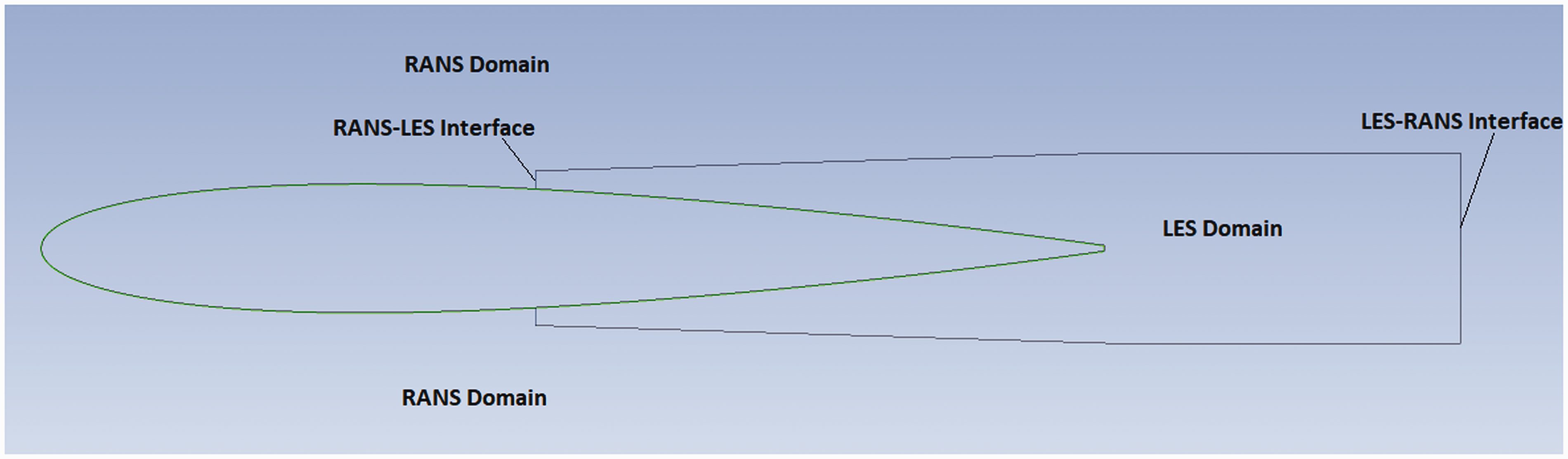

Non-conformal mesh generation

Multi-block structured mesh is firstly generated based on the whole domain and then divided into the RANS and the LES domain. The grid used in the RANS and the LES domain has to be conforming to the resolution requirements of the underlying turbulence models. Non-conformal mesh is generated at the RANS/LES interfaces to allow a refined grid in the LES domain. Typical RANS computations feature only one cell per boundary layer thickness in streamwise and spanwise directions. Typical LES requires mesh resolution with streamwise spacing of $x^{+}=10-100$ and spanwise spacing of $z^{+}\approx 20$ . To capture the boundary layer flow accurately, first cell wall normal spacing of $y^{+}<1$ is applied in both the RANS and the LES domain. The final mesh count is around four million hexahedral cells in total showing a significant reduction by a factor of approximate four compared to the wall-resolved LES method. ⁹ Mesh independence study based on the ELES simulation is performed.

The final mesh distribution at the mid-span plane for the whole domain and the local refined mesh in the LES domain are shown in Figure 2. The non-conformal mesh on the RANS-LES interface is shown in Figure 3.

Figure 2.

Mesh for the LES domain (left) and the entire domain (right).

Figure 3.

Non-conformal mesh on the RANS-LES interface – RANS side (left) and LES side (right).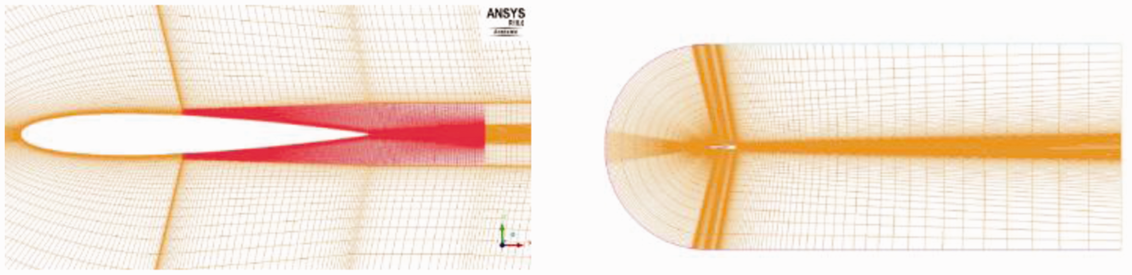

RANS/LES interface treatment

In the embedded LES domain, the top, bottom and downstream LES-RANS interfaces are treated as common interior zones. The most critical interface is the RANS-LES interface where the flow leaves the RANS domain and enters the LES domain. On the interface, the modelled turbulence kinetic energy in the RANS domain has to be converted into resolved energy in the LES domain by a turbulence generating method. Five classes of techniques of generating turbulent content at the RANS-LES interface have been developed, namely, precursor DNS/LES, turbulence recycling, synthetic turbulence generation, artificial forcing and vortex generation. ³¹ Vortex generation method is generally believed to be much quieter than all the other methods and is considered to be the most suitable turbulence generation method at the RANS-LES interface in aeroacoustic simulation. ³¹

Physically, vortex method is similar to those used in tripping boundary layer in experiments and can be used to trigger the turbulence development at the RANS-LES interface. Mathematically, the vortex method is based on the Lagrangian form of the 2D evolution equation of the vorticity ω which is given as below

$$\frac{\partial \omega }{\partial t}+(\overrightarrow{u}\nabla )\omega =\nu {\nabla }^2\omega$$

(2)

where the velocity vector is decomposed as

$$\overrightarrow{u}=\nabla \times \overrightarrow{\psi }+\nabla \phi$$

(3)

ψ is the 2D stream function and φ is the velocity potential. Taking the curl of this equation, one obtains

$$\omega =-{\nabla }^2\psi$$

(4)

The solution of equation (4) is given by the convolution of the vorticity with the 2D Green’s function

$$\psi (\overrightarrow{x})=-\frac{1}{2\pi }{\int \int }_{R^2}\mathit{ln}|\overrightarrow{x}-{\overrightarrow{x}}^{\text{'}}|\omega ({\overrightarrow{x}}^{\text{'}})\text{d}{\overrightarrow{x}}^{\text{'}}$$

(5)

This relation is used in equation (3) to yield the relation commonly known as the Biot–Savart law

$$u(\overrightarrow{x})=-\frac{1}{2\pi }{\int \int }_{R^2}\frac{(\overrightarrow{x}-{\overrightarrow{x}}^{\text{'}})\omega ({\overrightarrow{x}}^{\text{'}}).\overrightarrow{z}}{|\overrightarrow{x}-{\overrightarrow{x}}^{\text{'}}{|}^2}\text{d}{\overrightarrow{x}}^{\text{'}}$$

(6)

A particle discretization is used to solve the equation. These particles or “vortex points” are convected randomly and distributed randomly over the 2D face zone to generate turbulent fluctuations that needs to be specified at the RANS-LES interface. The vortex number that needs to be specified on the interface is related to the vortex size σ and the RANS-LES interface area A. The vortex size σ depends on the turbulence length scale L as below

$$\sigma =\frac{0.16\times L}{2}$$

(7)

$$L=\frac{k^{3/2}}{\varepsilon }$$

(8)

where k is the turbulence kinetic energy and ɛ is the turbulence dissipation rate. It is noted that the minimum vortex size is limited to the mesh size so that all the vortexes could be resolved properly. Assuming an ideal circular vortex is bounded by a square with length = height = σ, the vortex area is ${\sigma }^2$ and the maximum vortex number can be calculated as

$$n_{\text{max}}=\frac{A}{{\sigma }^2}$$

(9)

The vortex size σ on the RANS-LES interface is calculated from the initial RANS simulation and is shown in Figure 4. It can be seen clearly that there are two different scales of vortices on the interface. They are related to the near wall region, where the vortices are smaller by about one order, compared to the region away from the wall. For more realistic turbulence fluctuations generation, the RANS-LES interface is then split into two parts by means of a vortex size of $\sigma =0.0005\text{m}$ , resulting in one part near the wall and one part away from the wall. A mean vortex size is estimated by means of the mean turbulence length scale in each part of the interface, and then the mean vortex number could be calculated and applied on each part based on the corresponding vortex size and the interface area.

Figure 4.

Vortex size on the RANS-LES interface.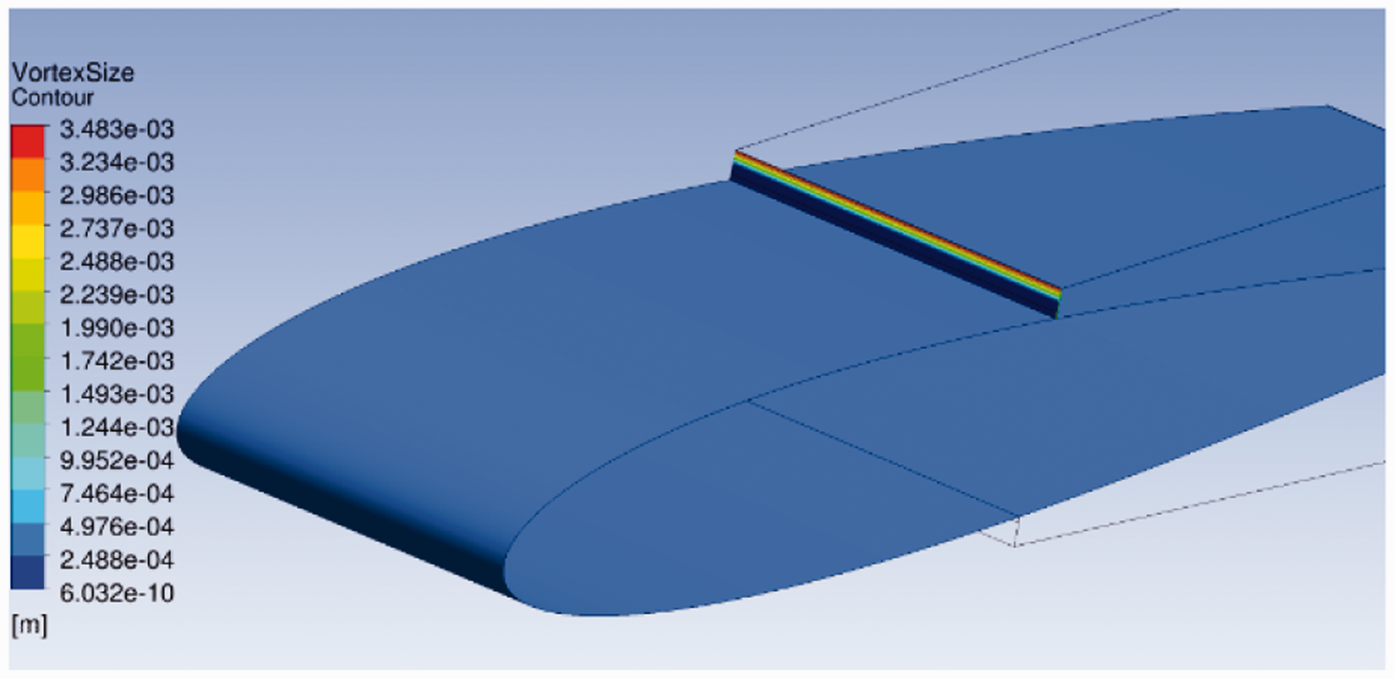

To verify the accuracy and efficiency of the splitting interface, two cases with and without interface split are tested. The surface pressure coefficient C_p for the two cases is presented and compared with the experimental data as shown in Figure 5. Here, C_p is defined as

$$C_p=\frac{P_{01}-P_s}{P_{01}-P_{s2}}$$

(10)

where P₀₁ is the inlet total pressure, P_s is the static pressure on the aerofoil surface and P_s2 is the outlet static pressure. This definition of the pressure coefficient accords with that in the experimental investigation. ³²

Figure 5.

Comparison of C_p for different RANS-LES interface treatment.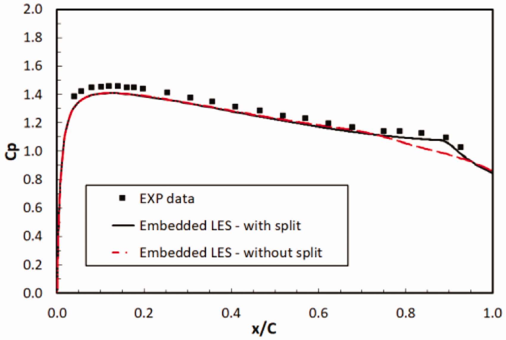

It can be seen that with the interface split, the boundary layer separation and transition are well predicted by the ELES. The C_p profile agrees well with the experimental data and the transition location with the maximum boundary layer displacement is predicted accurately. However, without the interface split, the artificial vortices are randomly distributed on the interface, resulting in unrealistic generation of the turbulence contents on the interface. It will alter the flow downstream in the LES zone globally, and thus eliminate the boundary layer flow separation and transition, as shown in Figure 5. Therefore, the interface split would enable more realistic vortices generation and distribution in the near wall region, where the initial instability waves and turbulence vortex are expected to develop, and thus produce more accurate results in the downstream LES simulation.

Turbulence modelling methods

The embedded LES allows combining the existing turbulence modelling and resolving technologies in a flexible way in the pre-defined RANS and LES zones. In this study, the classic LES with the wall-adapting local eddy-viscosity (WALE) subgrid-scale model is used in the LES domain. The WALE model is designed to return the correct wall asymptotic behaviour for wall bounded flows and a zero turbulent viscosity for laminar shear flows. It is suitable for the transitional flow simulation over the aerofoil.

It is advised that a separate RANS simulation is necessary to provide more realistic inlet conditions (velocity and turbulence profiles) at the RANS-LES interface. In this study, both k-ω SST fully-turbulent model and k-ω SST transition model have been tested in the RANS zone. The skin friction coefficient C_f is presented and compared in Figure 6, as an indicator for the boundary layer transition. It can be seen that, in fully-turbulent simulation, an early transition is predicted incorrectly (∼18% of the chord) upstream the LES zone due to the fully turbulent boundary layer assumption in the RANS zone. An abrupt drop of C_f at the RANS-LES interface (∼46% of the chord) implies the incorrect provision of the wall shear stress on the interface. However, with transition simulation in the RANS domain, C_f is transitioned continuously and smoothly across the interface and accurate wall shear stress is provided on the RANS-LES interface. Therefore, k-ω SST transition model is used in the RANS zone in this study in order to provide more accurate prediction on the boundary layer in the RANS domain and more physical RANS to LES transition on the interface.

Figure 6.

Comparison of C_f for different RANS model and interface treatment.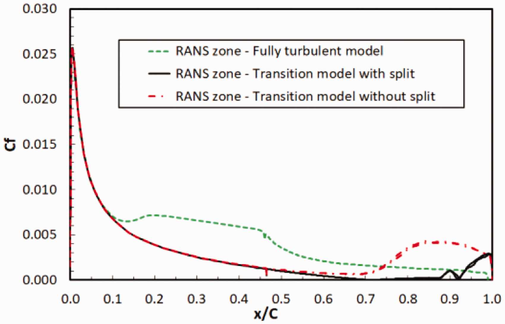

In addition, skin coefficient C_f for the two cases – with and without interface split is shown in Figure 6. It can be seen that with the interface split, the boundary layer separation and transition are observed near the trailing edge at the expected location. However, without the split, no separation takes place and the flow transition location moves upstream. This observation aligns with the C_p profile as shown in Figure 5.

Numerical scheme

In the RANS zone, second-order upwind discretization scheme is employed and pressure-velocity coupling scheme is used to solve the averaged Navier–Stokes governing equations. In the LES zone, bounded central differencing method is used for momentum spatial discretization. Large turbulence scales are resolved directly and small turbulence scales are modelled by the WALE subgrid-scale model. For transient discretization, bounded second-order implicit method is used in the whole domain. The commercial CFD solver, Fluent 18.2, is used for all of the simulations.

Results and discussion

An initial RANS simulation with $k-\omega \mathit{SST}$ transition model for the entire domain is performed. Once the RANS simulation gets reasonably converged, it is converted to unsteady RANS/LES simulation, in which $k-\omega \mathit{SST}$ transition model is kept in the RANS domain and LES + WALE model is used in the LES domain. Ten flow-through time based on the freestream velocity and the aerofoil chord length have been run to ensure the initial turbulent flow field is settled down fully. Turbulence samples are then collected with the turbulence flow averaging process for another 20 flow-through time.

The key flow characteristics around the NACA0012 aerofoil are collected and presented in the following sections. Comprehensive validation of the ELES results is performed by comparing with the experimental data and the wall-resolved LES results. Evaluation of the capability and performance of the ELES method in aerodynamics and aeroacoustics application is discussed in terms of accuracy, computational cost and complexity of implementation.

Transitional boundary layer flow development

The static pressure on the upper and lower surface of the aerofoil is averaged in time and its distribution is defined by pressure coefficient C_p, as defined in equation (10). The comparison between the calculated C_p and the experimental data is presented in Figure 7, together with the result from the inviscid flow calculation.

Figure 7.

Surface pressure coefficient on the aerofoil.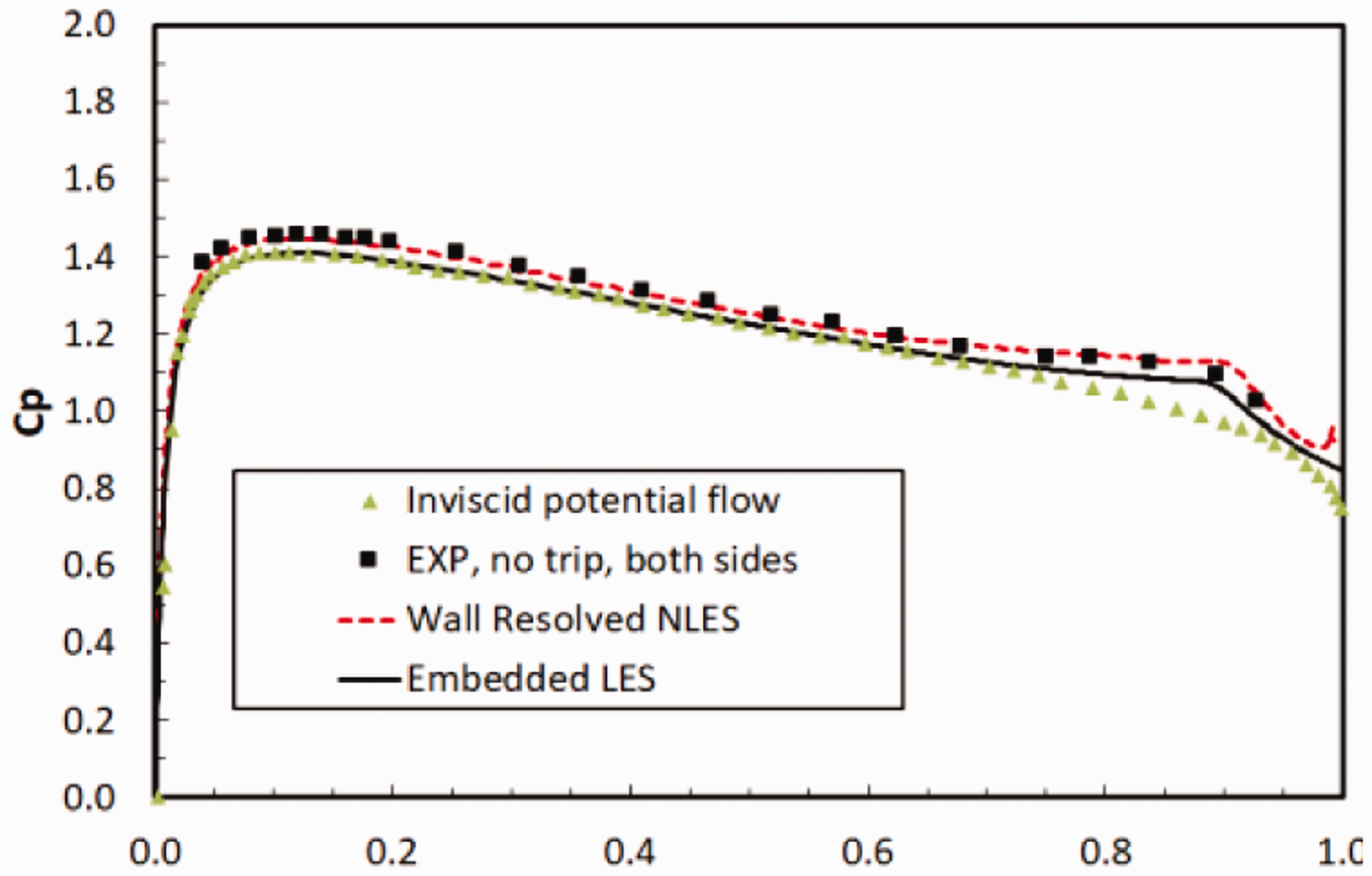

It can be seen that the pressure coefficient C_p from the ELES simulation agrees very well with the experimental data. As expected, the boundary layer is developed on the aerofoil surface and behaves as laminar flow up to 65% of the chord length ( $x/C=0.65$ ). After that, the boundary layer starts to separate until near the end of the aerofoil ( $x/C=0.97$ ), resulting in a separation bubble in the vicinity of the trailing edge as observed in the experiments. It is predicted that the boundary layer transition is undergoing in this area due to the laminar flow separation. The boundary layer reattaches afterwards at the very end of the aerofoil indicating the formation of turbulent boundary layer. It can be seen that the boundary layer flow separation and the reattachment afterwards are captured accurately in the ELES, while the value of C_p is slightly under-predicted by the ELES over the first half of the aerofoil.

Boundary layer thicknesses associated with different boundary-layer regimes were measured and analysed in the experimental investigation. ³² In the computational study, the boundary-layer thickness δ has been integrated from the analysis of the mean streamwise velocity profiles. The velocity at the edge of the boundary layer U_e was defined at the point where the velocity was 99.5% of the freestream velocity. The displacement thickness ${\delta }^{*}$ , the momentum thickness θ and the shape factor H are defined in equations (11) to (13)

$${\delta }^{*}={\int }_{y=0}^{\delta }(1-\frac{u(y)}{U_e})\text{d}y$$

(11)

$$\theta ={\int }_{y=0}^{\delta }\frac{u(y)}{U_e}(1-\frac{u(y)}{U_e})\text{d}y$$

(12)

$$H=\frac{{\delta }^{*}}{\theta }$$

(13)

The shape factor is then calculated and presented in Figure 8. The experimental data and the wall-resolved LES results are plotted together for comparison. At streamwise location of $x/C=0.4$ , the values of $H=2.4$ for the wall-resolved LES and $H=2.8$ for the ELES match the value of $H=2.6$ measured in the experiments. For Blasius boundary layer, $H=2.59$ is a typical value of laminar flow. ³⁵ The value of the shape factor increases towards the separation point, reaching a value of $H=3.67$ for the wall-resolved LES at $x/C=0.6$ and $H=3.5$ for the ELES and $H=3.25$ for the experiments at $x/C=0.65$ . A typical value of H in a separated laminar boundary layer is approximately 3.5. ³⁶ As Hatman and Wang ³⁷ reported, H reaches a maximum value in the region around the maximum displacement $x_{\mathit{MD}}$ of the separated shear layer. From Figure 8, it is evident that this occurs at $x_{\mathit{MD}}/C=0.86$ with a maximum value of $H\approx 4.7$ from both the experiment and the ELES, while the wall-resolved LES overpredicted the boundary layer separation and its maximum value of H reaches 5.5. Downstream the maximum displacement point, transition is undergoing, the boundary layer flow becomes turbulent and reattaches upstream of the trailing edge quickly. Accordingly, the shape factor H decreases sharply after the maximum displacement towards the trailing edge to a value around $H\approx 1.8$ from all the simulations and the experiment measurement. Overall, the ELES performs better than the wall-resolved LES in terms of H factor. Both the trend of the boundary layer development and the value of the boundary layer thickness match the experimental data. It is concluded that the ELES method is capable of capturing the flow features in different boundary layer regimes over the NACA0012 aerofoil at the moderate Reynolds number of ${\mathit{Re}}_c=2\times {10}^5$ . The predicted separation point, reattachment point and the maximum displacement point and the corresponding boundary layer thickness match the experimental data well.

Figure 8.

Boundary layer shape factor on the aerofoil.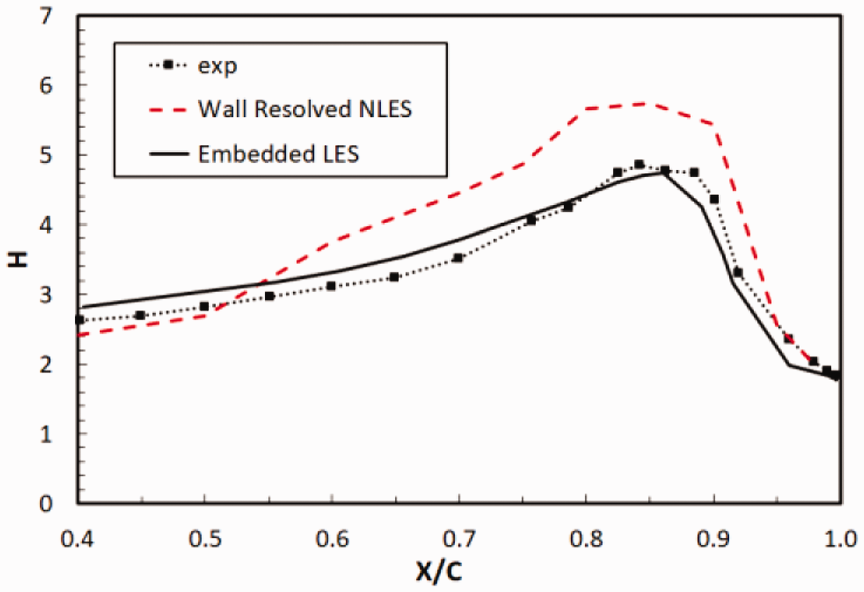

In the experimental data and the numerical prediction, transition takes place further downstream of the separation starting point, in the region of the maximum displacement at $x/C=0.86-0.88$ . According to Hatman and Wang, ³⁷ this is a typical laminar separation – short bubble transition mode, dominated by the Kelvin–Helmholtz (K–H) instability. In Figure 9, the plot of the mean velocity streamlines around the aerofoil trailing edge shows the laminar boundary-layer separation on both the top and bottom sides and the recirculation bubbles that formed. It indicates clearly that the laminar separation – short bubble transition mode takes place in the boundary layer.

Figure 9.

Mean velocity streamlines around the aerofoil trailing edge.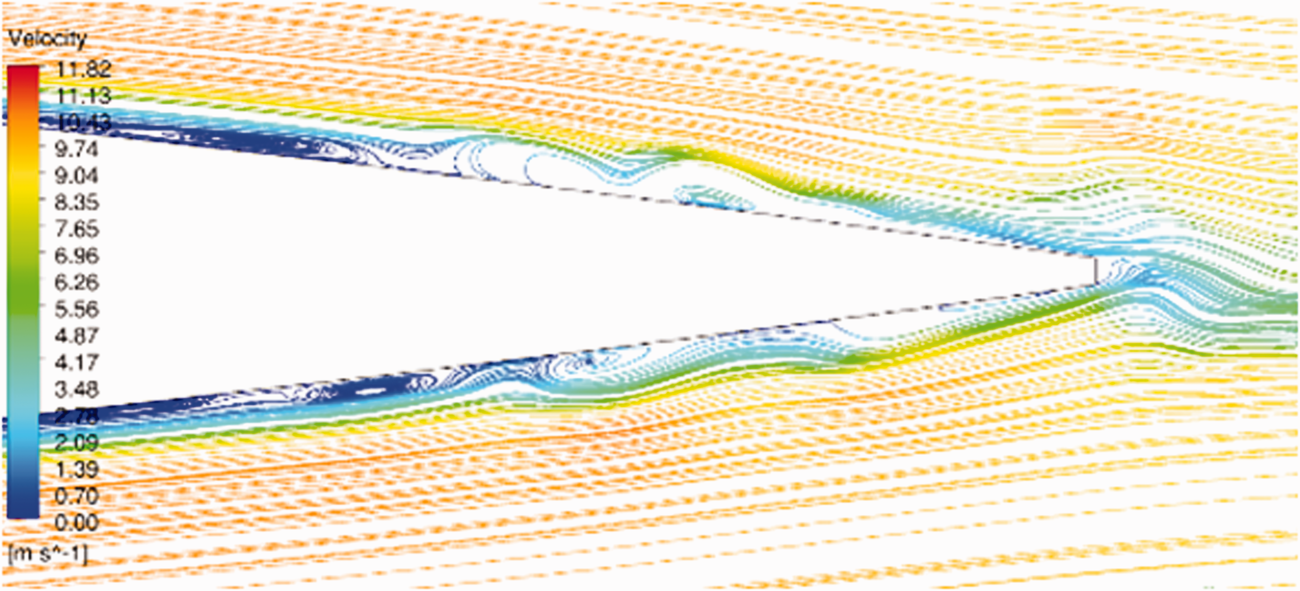

To examine the transitional and separated boundary layer further, the streamwise mean velocity U_m and the root-mean-square ( $\mathit{rms}$ ) field of velocity fluctuations $U_{\mathit{rms}}$ in the boundary layer are presented in Figure 10. Three representative locations in the boundary layer corresponding to the laminar flow regime ( $x/C=0.55$ ), the separation/transitional flow regime ( $x/C=0.86$ ) and the reattachment/turbulent flow regime ( $x/C=0.98$ ) are chosen. Again, the numerical results from the wall-resolved LES and the experimental data are plotted together for comparison. Both the mean velocity and the rms velocity are rescaled by the local external freestream velocity. Dimension Y in Figure 10 is the vertical distance away from the aerofoil surface.

Figure 10.

Mean and rms streamwise velocity profiles in the boundary layer.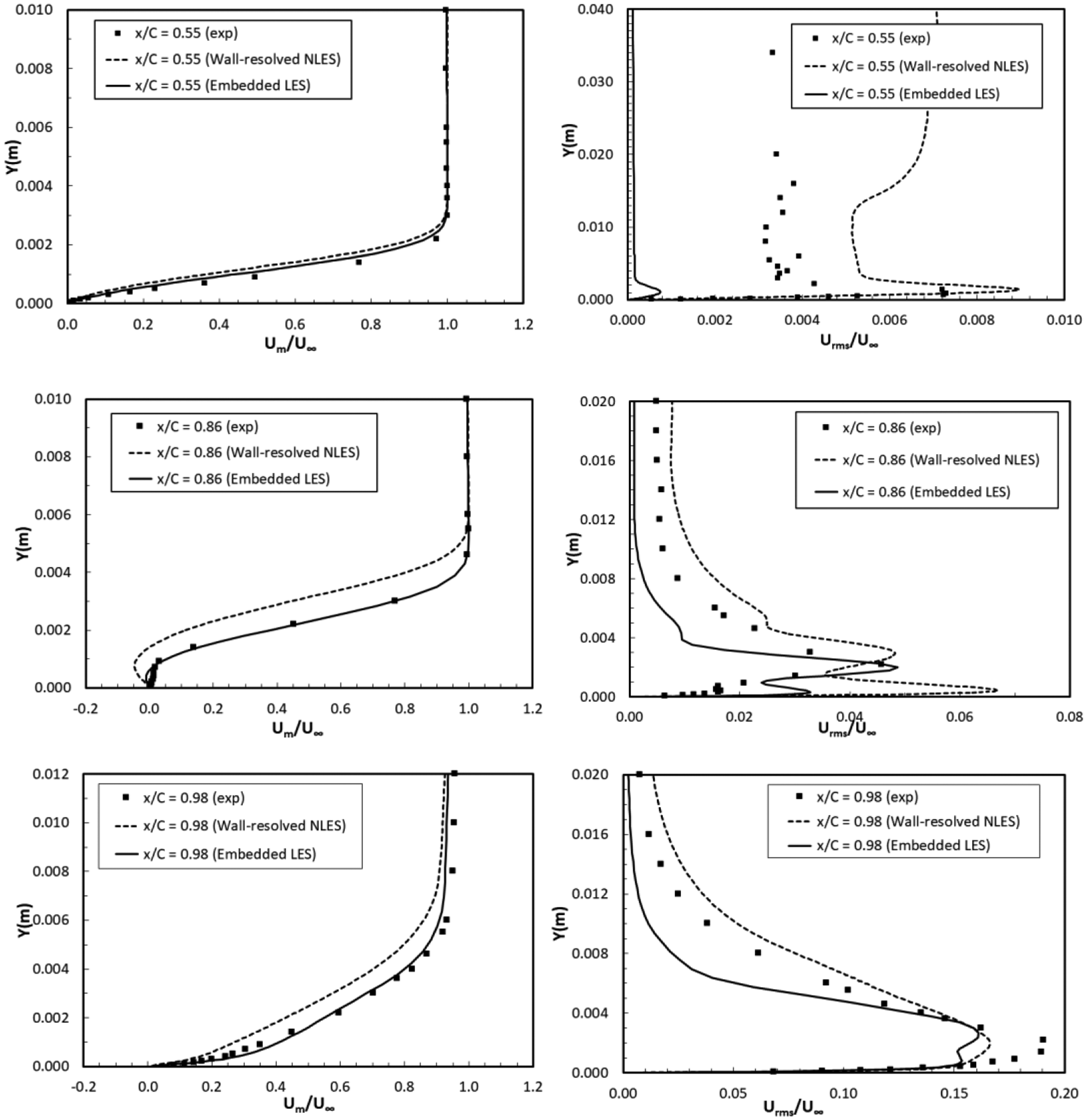

As shown in Figure 10, at the streamwise location of $x/C=0.55$ , the mean velocity distribution in the boundary layer presents a typical laminar flow profile with a thin boundary layer ( $\delta \approx 2.5\text{mm}$ ) and a small turbulence intensity level ( $U_{\mathit{rms}}<0.01$ ). At the location of $x/C=0.86$ , the boundary layer undergoes separation and reaches its maximum displacement point. The mean velocity distribution presents a transitional flow profile with an increased boundary layer thickness ( $\delta \approx 5\text{mm}$ ) and reversed flow in the near wall area. The turbulence intensity level is increased with a maximum value of $U_{\mathit{rms},\text{max}}\approx 0.05$ in the near wall region. Towards the trailing edge, at the location of $x/C=0.98$ , a typical turbulent boundary layer profile is presented with a much thicker boundary layer ( $\delta \approx 12\text{mm}$ ) and a much higher turbulence intensity level with $U_{\mathit{rms},\text{max}}\approx 0.15-0.2$ .

Comparing the experimental data and the numerical results in Figure 10, it can be seen that the mean velocity profiles from the ELES method agree very well with the experimental measurement in all three flow regimes. The ELES presents improved accuracy compared to the wall-resolved LES. The latter over-predicts the boundary layer thickness resulting in a stronger boundary layer separation and a larger displacement downstream ( $\frac{x}{C}=0.86$ ) until the flow reattachment matches the shape factor profile as shown in Figure 8. For the rms velocity, neither the ELES nor the LES can predict the profile very well. In all three flow regimes, the ELES under-predicts the turbulence intensity level in the boundary layer, while the wall-resolved LES over-predicts it in the laminar and the transitional regimes. Hatman and Wang ³⁸ found that the maximum value of the rms velocity for the separation-induced transition mode was approximately 0.18, which is similar to the numerical prediction of 0.17 from the wall-resolved LES and 0.16 from the ELES, found in the region around the reattachment point of $x/C=0.98$ .

It is noted that the directional insensitivity of hot-wire anemometry employed in the measurements of the boundary-layer velocity profiles resulted in distorted mean velocity profile in experimental measurement, which causes the significant disagreement between the numerical results and the experimental data in terms of the near-wall velocity distribution, as illustrated in Figure 10 at the location of $x/C=0.86$ .

Wall-normal mean velocity V_m and root mean square of its fluctuation $V_{\mathit{rms}}$ are also presented at the location of $x/C=0.98$ , as shown in Figure 11. It can be seen that, in the near wall region, the embedded LES performs better than the wall-resolved LES, showing a good agreement with the experimental data. However, in the region away from the wall, both methods deviate from the experimental data. Overall, the ELES method provides more accurate prediction of mean and rms velocity profiles than the wall-resolved LES method.

Figure 11.

Mean and rms wall-normal velocity profiles.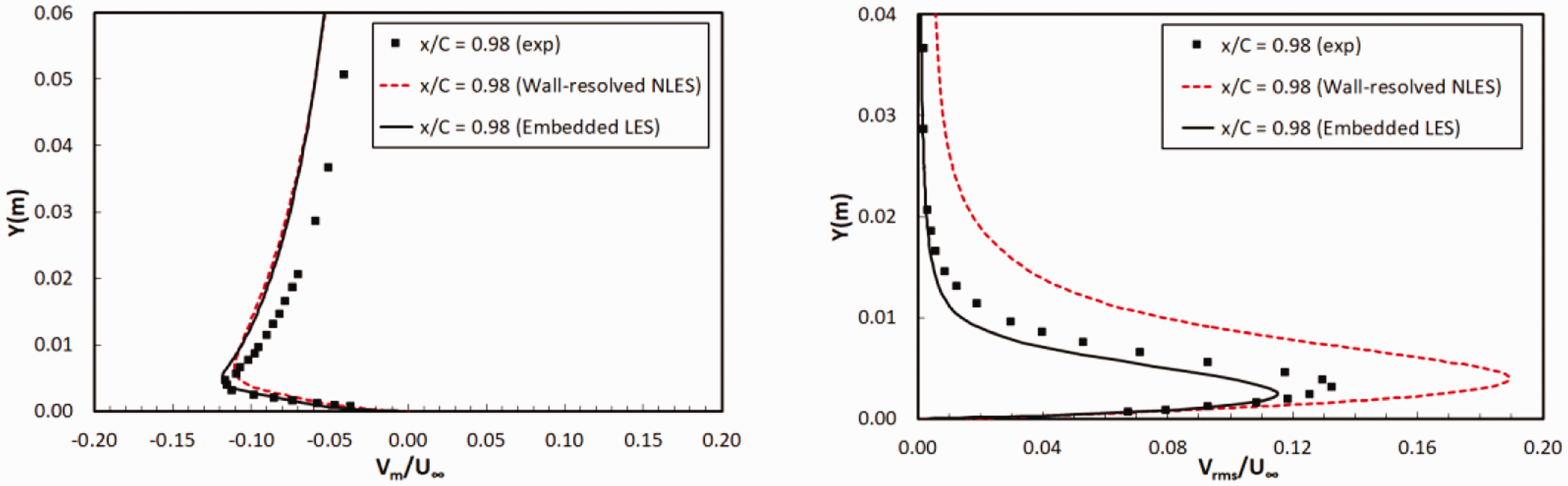

Turbulence development near aerofoil trailing edge

It has been identified that the unsteady turbulent fluctuation in the near-wall area around the aerofoil trailing edge is the main source for the aerofoil trailing edge noise generation.^9,32 Therefore, the turbulence development and its characteristics predicted by the ELES method will be presented and validated in this section.

One of the favourable ways to visualize the turbulent vortical structures around aerofoil trailing edge is using Q-criterion. It represents the balance between the rate of vorticity and the rate of strain, which is as expressed as follows

$$Q=\frac{1}{2}({\Omega }_{\mathit{ij}}{\Omega }_{\mathit{ij}}-{\text{S}}_{\mathit{ij}}{\text{S}}_{\mathit{ij}})=\frac{1}{2}\frac{{\nabla }^{2}p}{\rho }$$

(14)

where ${\Omega }_{\mathit{ij}}$ and ${\text{S}}_{\mathit{ij}}$ are the anti-symmetric and symmetric part of the velocity gradient respectively with the following expression

$${\Omega }_{\mathit{ij}}=\frac{1}{2}(\frac{\partial u_i}{\partial x_j}-\frac{\partial u_j}{\partial x_i})S_{\mathit{ij}}=\frac{1}{2}(\frac{\partial u_i}{\partial x_j}+\frac{\partial u_j}{\partial x_i})$$

(15)

In the core of a vortex $Q>0$ , vorticity increases as the centre of the vortex is approached. Thus, the regions of positive Q-criterion correspond to vortical structures. The contour of the iso-surface of Q-criterion with $Q=20,000$ coloured by turbulence vorticity magnitude is presented in Figure 12. It is found that towards the aerofoil trailing edge, the rolling-up of two-dimensional turbulent eddies is observed due to boundary-layer flow separation and transition. It progressively becomes three-dimensional at the blunt trailing edge and propagates forward into the wake flow in a very chaotic manner. The turbulence development length and width scales are clearly visualized.

Figure 12.

Contour of vorticity magnitude on iso-surface of Q criterion, 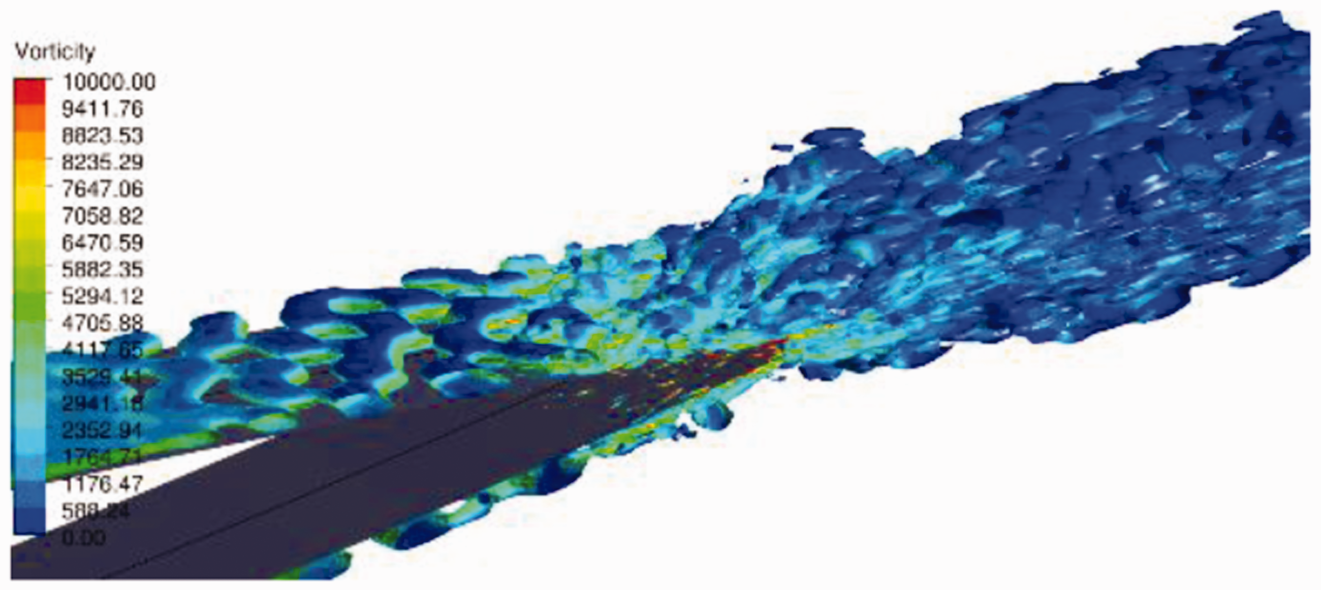$Q=20,000$ .

In Figure 13, the iso-surface of the vorticity magnitude is plotted coloured by the mean streamwise velocity. It can be seen that the vortices are developed within the boundary layer as they approach the aerofoil trailing edge, and propagate downstream and shed at the blunt trailing edge. In the vicinity of the trailing edge, a deep re-organization of the turbulent structure occurs.

Figure 13.

Iso-surface of vorticity magnitude coloured by the mean streamwise velocity.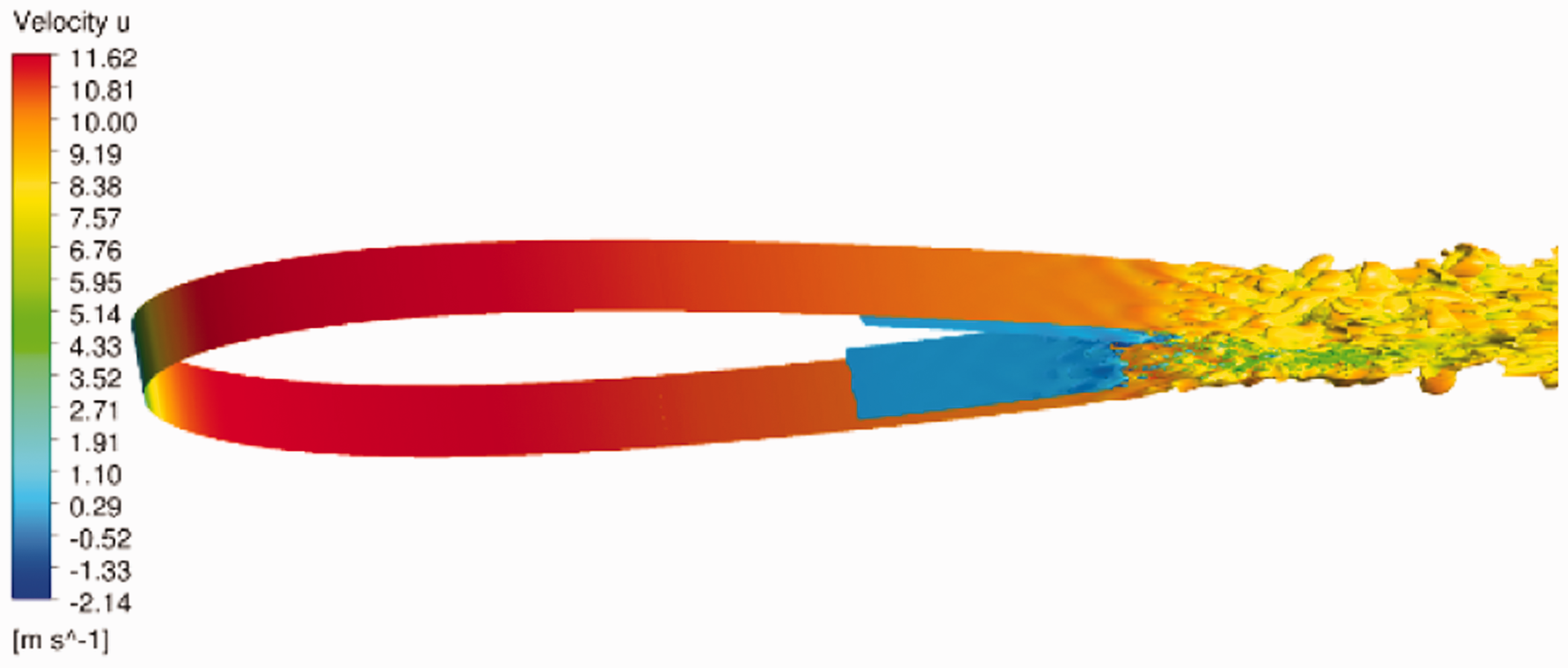

The turbulence development demonstrations here align with the observation in the experiment and the prediction from the wall-resolved LES. It indicates that the ELES method is capable of predicting the turbulent fluctuation in the near field around the aerofoil trailing edge; therefore, it is suitable for the noise source strength computation around aerofoil trailing edge.

Wake flow development

Wake flow development behind the aerofoil is examined in this section. In the experiment, velocity and turbulence profiles in three wake positions, $\frac{x}{C}=1.01,1.02\hspace{1em}\text{\hspace{1em}and\hspace{1em}}\hspace{1em}1.05$ are measured. Therefore, the mean streamwise velocity distribution and rms of the velocity fluctuations at the same locations from the embedded LES are presented and validated in Figure 14. Both velocities are scaled by the freestream velocity in the far field. It is noted that the velocity profiles present turbulence energy and momentum deficit in the wake flow.

Figure 14.

Mean and rms streamwise velocity profiles in the wake flow.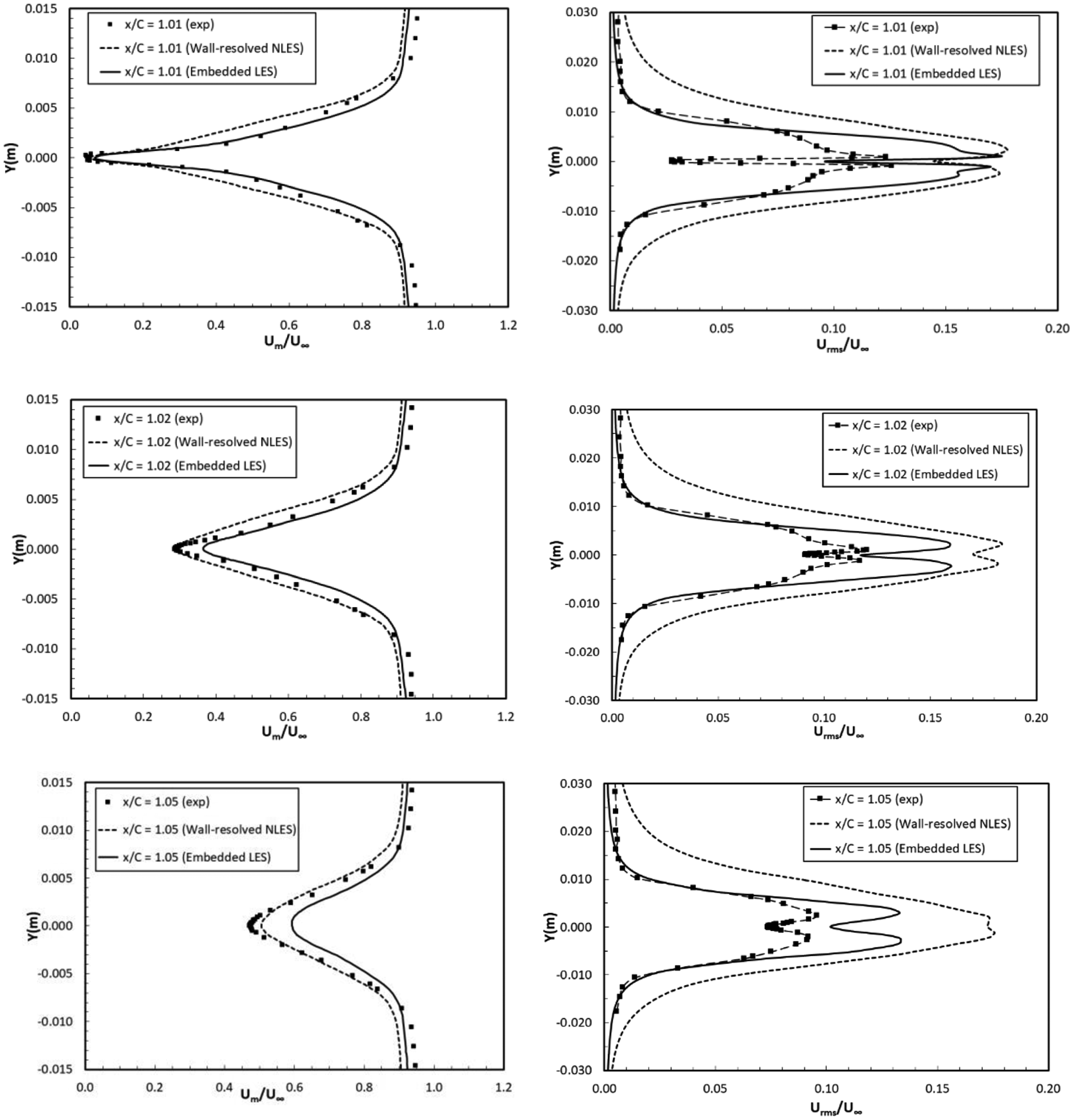

Due to the large trailing edge thickness, the wake flow velocity can reach very small values in the vicinity of the extended trailing edge central line, as shown at the wake location of $x/C=1.01$ in Figure 14. The rms velocity profile at this location shows two peaks with a sharp minimum between them, which may be related to the presence of a quasi-periodic unsteady vortex shedding from the blunt edge. It is noted that the thickness of the blunt trailing edge (1.6 mm) is the scale of the trailing edge quasi-periodic vortex shedding. Further downstream of the blunt trailing edge, the minimum values of the mean velocity and the rms velocity increase accordingly.

Comparing the experimental data and the computational results in Figure 14, it is found that at the location of $x/C=1.01$ , the ELES performs better than the wall-resolved LES. The mean velocity from the ELES simulation matches the experimental data very well. The minimum velocity appearing in the vicinity of the extended central line of the aerofoil is accurately predicted. The expansion of the wake flow velocity profile downstream the aerofoil trailing edge aligns with the experimental data. However, at the other two locations, the wall-resolved LES performs better than the ELES in terms of the minimum value of the velocity. The embedded LES under-predicts the momentum deficit in wake flow and the flow velocity is recovered much quicker than that in the wall-resolved LES at the locations of $\frac{x}{C}=1.02\hspace{1em}\text{\hspace{1em}and\hspace{1em}}\hspace{1em}1.05$ . For the rms of velocity fluctuations, both the ELES and the wall-resolved LES over-predict the turbulence energy values; however, the expansion of the rms velocity profile is predicted accurately in the embedded LES, while the wall-resolved LES over-predicts it significantly.

The wall-normal mean and rms velocity distribution in the wake flow at the location of $x/C=1.01$ are presented in Figure 15 together with the wall-resolved LES results and the experimental data for comparison. It can be seen that both the wall-resolved LES and the ELES results are in a good agreement with the experimental data in terms of the wall-normal mean velocity in the near wall region, while both under-predicts the mean velocity in the area away from the wall. For the rms velocity profiles, the ELES performs better than the wall-resolved LES showing two peaks with a sharp minimum between them, which matches the experimental data. However, the wall-resolved LES presents three peaks with two minimum values. Both the ELES and the wall-resolved LES under-predicts the rms velocity.

Figure 15.

Mean and rms wall-normal velocity profiles in the wake flow.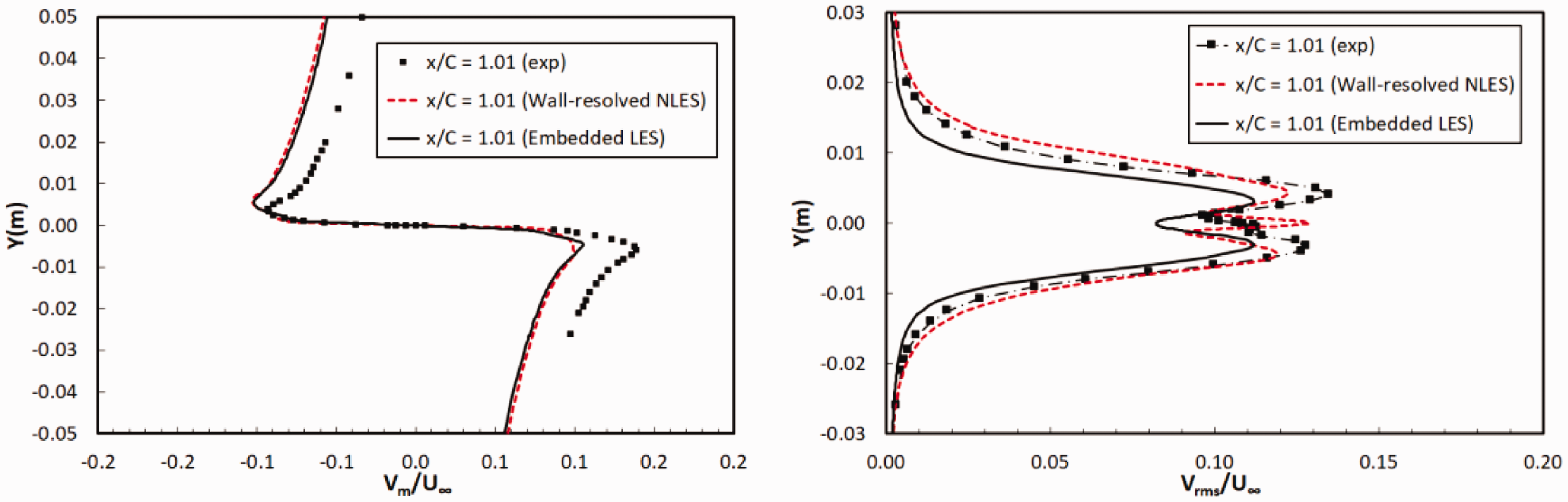

Conclusions

An accurate computational simulation for the near-field turbulent flow around aerofoil trailing edge is of outstanding importance for aerodynamic noise prediction. The aerofoil trailing edge noise has been identified as a significant contributor to fan noise and airframe noise.

In this study, a zonal hybrid RANS/LES method, called embedded LES, is implemented for the separation-induced transitional flow simulation around NACA0012 aerofoil trailing edge at a moderate Reynolds number. It aims to evaluate the capability of the ELES method in aerodynamics and aeroacoustics applications for wall-bounded aerospace flow.

Some good practice on implementing the zonal ELES method in transitional flow over aerofoil is detailed, including the definition of the RANS and LES sub-domain, non-conformal mesh generation, RANS-LES interface treatment, turbulence modelling methods in the RANS and LES zone, and the numerical discretization schemes. Particularly, the RANS-LES interface is split according to the different vortex size scale, and different vortex numbers are applied in the regions of near the wall and away from the wall. This special interface treatment guarantees a more realistic generation and distribution of the artificial turbulence fluctuations on the RANS-LES interface. Transition turbulence modelling method in the upstream RANS zone improves the accuracy of the LES inflow. Both practices improve the simulation accuracy in the downstream LES zone.

A comprehensive validation of the ELES results is performed by comparing with the experimental data and the wall-resolved LES results, in terms of transitional boundary layer flow development, turbulence development near aerofoil trailing edge and wake flow development. The capability of the zonal ELES method in wall-bounded aerospace industrial flow application is assessed in terms of its accuracy, computational cost and complexity of implementation.

Accuracy

The ELES results agree well with the experimental data in predicting the unsteady flow features, boundary layer separation and transition, and turbulence development near the aerofoil trailing edge. The predicted surface pressure distribution and the boundary layer thickness agree very well with the experimental data. The velocity distribution in three typical boundary layer regimes – laminar, transitional and turbulent – is well predicted, as well as the turbulence momentum deficit in the wake flow. The turbulence energy (rms of the velocity fluctuation) in the boundary layer and the wake flow is predicted in an agreeable range compared to the experimental data. Overall, the ELES method can provide the same level of accuracy as the wall-resolved LES method. For some of the unsteady flow characteristics, the ELES method performs even better than the wall-resolved LES method, such as the transitional boundary layer development and the velocity distribution in the boundary layer. It is concluded that the ELES method is suitable for the transitional turbulent flow simulation around aerofoil trailing edge for the purpose of aerodynamic noise source prediction.

Computational cost

In the present study, the embedded LES is run based on a second-order numerical scheme and a non-conformal mesh of 4M, while the wall-resolved LES is carried out based on a sixth-order scheme and a refined mesh of 16M. ⁹ Clearly, the computational cost of the ELES method is reduced significantly compared to the wall-resolved LES method due to the reduced LES domain and the less mesh size. However, at the RANS-LES interface, the modelled turbulence kinetic energy has to be converted into resolved energy by turbulence generating methods, which needs extra computing effort and time, while the reduced LES domain will ease the computing effort compared to the wall-resolved LES over the entire domain. A reduction factor of approximately four in computing CPU time is achieved without altering the accuracy. However, compared to the RANS method, the ELES method is still computationally expensive.

Complexity of implementation

To implement the embedded LES method, it is necessary to pre-define the RANS and the LES domain by the user, generate the non-conformal mesh at the RANS/LES interfaces and provide special treatment on the interface, all of which will result in extra work comparing to the pure LES method. Regarding the turbulence modelling and the numerical scheme, the ELES method is literally a combination of existing models/technologies in a flexible way in the RANS and the LES zone, so it will not cause any extra complexity. In summary, apart from the extra work on pre-defining the LES domain shape and size as well as the RANS-LES interface treatment, the ELES method has similar or even less level of implementation complexity as those in the pure LES methods.

The successful implementation of the ELES method in this study provides a computationally efficient approach for hybrid aeroacoustic simulation with sufficient accuracy. It is proved to be a promising approach for industrial flow applications involving wall boundary layer due to its significant computational efficiency. This study is not the first attempt to implement the ELES method in aerofoil trailing edge noise source generation, but it is the first one to implement it in a transitional boundary layer flow simulation. The separation-induced transition and the resulting turbulent flow development around aerofoil trailing edge are accurately predicted by the ELES, which makes the present study a good source of validation with some good practice for any further similar investigations.

The recommendation for next stage work is to validate the embedded LES method in more complex aerospace industrial flow application, such as the high-lift configuration. Also, further work on improving the LES inflow conditions is needed, particularly for its aeroacoustic application. According to Shur, ³¹ a “sudden” formation of strong vortical structures accompanied with an unsteady mass source at the RANS-LES interface would generate spurious noise and the risk of drastically corrupting the genuine aerodynamic noise of the flow. Therefore, special acoustically oriented modifications of the existing turbulence generation methods are needed to suppress the spurious noise sources at the RANS-LES interface.