
Abstract
In-service railway vehicles are increasingly used for autonomously monitoring railway track condition with no disruption to passenger and freight timetables. However, comparison of track geometry recordings with inspection measurements from Track Recording Vehicles (TRVs) can be challenging due to longitudinal misalignment of recording data. Following review of existing literature on challenges of recording alignment, a method for autonomously correcting the longitudinal alignment of track geometry monitoring recordings with reference inspection data is presented which makes use of Hidden Markov Models (HMMs). This methodology is robust to estimation errors and can produce global alignment to known track sections with minimal constraints provided. Recordings taken from a section of high-speed rail line in the United Kingdom validate the methodology. Results indicate that one journey per 32 hours can be correctly and autonomously aligned to the reference, enabling more frequent monitoring of track geometry degradation at a lower cost than monthly TRV inspections can permit. The technique scales to larger fleets of instrumented vehicles to provide wider and more frequent network coverage.
Keywords
Introduction
Condition monitoring of railway track geometry is essential for ensuring safe and reliable operation of passenger and freight train services. Inspection and monitoring of railway track condition are critical albeit costly responsibilities for railway infrastructure managers.
Stakeholders must quickly assess relevant information from large (and growing) volumes of data generated from increasingly sophisticated methods for inspecting and monitoring track condition. Infrastructure managers compare recording data with prior measurements to measure the deterioration in railway track quality over time. Line-side or vehicle-mounted sensors provide measurements, with current industry best-practice relying on inspection using Track Recording Vehicles (TRVs), though there is increasing use of instrumented in-service vehicles for track condition monitoring.
Both types of track geometry recordings—inspection and monitoring—exhibit errors in positional along-track alignment when compared with other recordings for the same section of track (see Figure 1). These errors can be significantly larger for recordings from in-service vehicles, for which the starting position and route are not known in advance. Example comparison of Unaligned (left) and Aligned (right) recordings for HS1 (North Section).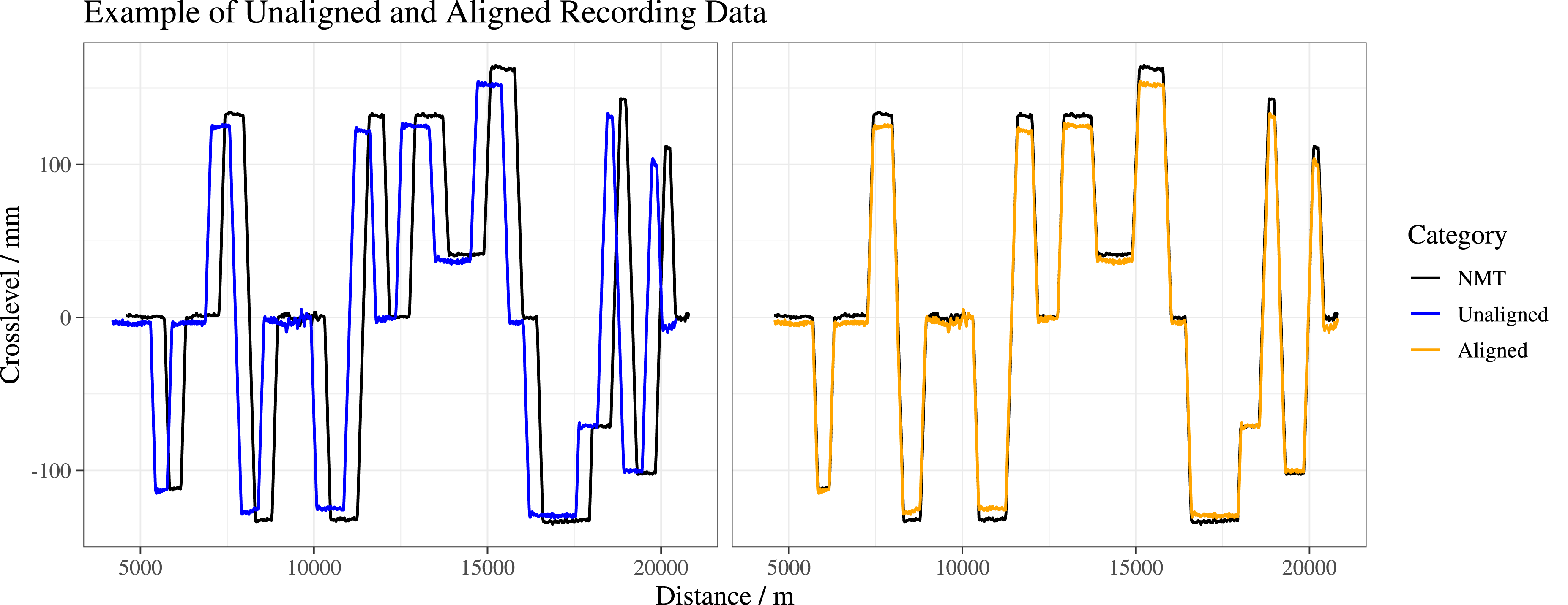
This paper presents a comprehensive review of track geometry recording alignment methods alongside detailed discussion of aligning track geometry recordings from in-service vehicles, followed by presentation of a methodology for reliable general-case alignment of these recordings. Recording data from a vehicle operating on the High Speed 1 (HS1) line in Kent, UK forms the basis of a case study. These results are discussed and improvements on the initial methodology are explored. Finally, conclusions and recommendations for future work are presented.
Background
Track geometry is recorded using numerical measurements describing 3-dimensional variation of left, right and combined rail positions. Combined measurements form a Track Quality Index (TQI) which reports the variation of track geometry parameters over given lengths of track. 1 These sections may be overlapping, grouped according to their characteristics, or defined in an ad-hoc manner. Repeated track geometry measurements of the same sections of track can be compared allowing change in track condition to be reported.
Track inspection
Infrastructure managers must accurately assess the condition of track in order to ensure that its condition is safe to allow passage of railway vehicles.
Data from TRVs includes position along the track and velocity of the measurement vehicle at point of measurement, along with recordings of primary track geometry parameters (crosslevel/cant, vertical irregularity/top and lateral alignment) and secondary track geometry parameters (twist, cant deficiency).
Network Rail, the national UK infrastructure manager, reports data points from their TRVs at a fixed interval in the distance domain: every 0.2 m. Vertical irregularity and lateral alignment are reported over a wavelength (35m or 70m) while twist is reported over lengths of track (3m and 5m).
A single set of recording data (henceforth referred to as a journey) is reported alongside identifying metadata. This includes the recording date, Engineer’s Line Reference (ELR) code and Track ID (TRID) code. The latter two are, respectively, used to identify the route along with individual running lines e.g. Up Main (towards London) or Down Main (away from London) and, together, allow the specific section of track covered by the recording train to be identified in an asset database.
TRVs in use worldwide include Japanese ‘Doctor Yellow’ inspection vehicles for Shinkansen high-speed lines, 2 Network Rail’s New Measurement Train (NMT), 3 China’s CJ-4G 4 and Austrian Railways’ track recording coach. 5 All vehicles record track geometry parameters at regular distance intervals, typically 0.20–0.25 m.
There are limitations in the use of TRVs. They are expensive to purchase and operate and consume train paths in the timetable. As a result, the minimum typical inspection period for a line in the UK is 4 weeks. 6
Track monitoring
Methods of acquiring track geometry data have been developed which do not rely on running dedicated vehicles, instead relying upon instrumenting in-service trains with Inertial Measurement Units (IMUs): research from the University of Birmingham, 7 Italy, 8 Japan 9 and others, Spain, 10 and India. 11
Inertial measurement units can provide estimation of common parameters used in TQIs: vertical irregularity, 12 lateral alignment, 13 and crosslevel.7,14 Gauge cannot be measured using purely inertial methods.
Other sensors can be fitted to in-service trains, with optical sensors able to provide better estimation of gauge and lateral alignment. 15 These require a higher maintenance frequency due to accumulation of dirt affecting measurements.
While the frequency at which in-service vehicles traverse tracks is an advantage over TRVs, there are limitations. Passenger and freight services slow down, accelerate, or stop frequently, which affects track geometry estimation accuracy. 16 It may not be possible to install sensors in an optimal position on the train. Finally, route taken by trains through the network and starting and ending positions are not known in advance.
Comparison of track geometry inspection and monitoring
Inspection is performed using TRVs and is used for decision making on safety-critical interventions, thus data must be accurate and robustly aligned. TRVs are typically attended by operators who provide input as to which section of track that the vehicle is traversing.
Conversely, in-service vehicle-based monitoring is unattended and provides no information on which track is being traversed. Monitoring can be undertaken using inexpensive sensors on in-service vehicles and is not typically relied upon for safety-critical decision making, instead used to monitor degradation of track sections which may benefit from preventive maintenance or further inspection.
Recording alignment
Distance traveled by recording vehicles is typically estimated by tachometer. 17 These sensors are inaccurate in poor adhesion or high traction conditions due to wheel slip and slide and require re-calibration due to wheel wear. 18 Algorithms can compensate for wheel slip in distance estimation19–21 which require sophisticated onboard processing but cannot remove uncertainty entirely.
TRVs are designed and built with tachometers installed, however in-service vehicles may not have them fitted. Tachometer installation is intrusive and, while new trains will likely be equipped with tachometers for train control purposes, this data may not be available to condition monitoring teams. Avoiding tachometer installation would enable more widespread condition monitoring of railway track through fitting IMUs to older rolling stock.
Accurate distance estimation is critically important in comparing journeys to determine possible changes in track geometry. Assuming perfect sensors, acquisition processes and track alignment, as well as perfect knowledge of origin position within the track network, multiple journeys will overlap in the along-track longitudinal (x) domain, measurements of the same sections of track will be coincident and there will be no discrepancies requiring correction.
These conditions are not possible and some degree of automatic or manual alignment is required to correct x positions of data points from journeys to ensure they correspond to previous journeys. Successive recordings may exhibit linear or non-linear shifts in their x values of 1 mm to 1m per km, with larger non-linear shifts more likely for recording data acquired without tachometer availability. Other reasons for misalignment may include differing start locations for vehicles, differences in vehicle dynamic properties, errors in distance estimation or irregularities in the track itself.
Monitoring data alignment faces challenges not seen in inspection data alignment. These include unknown starting location, as inspection trains begin from known locations, no knowledge of planned journey, as inspection trains operate along planned routes known by operators, and a need to reject journeys not relevant for monitoring purposes e.g. depot movements.
A global alignment considers all possible positions for a specific recording, whereas a local alignment has prior knowledge about where a recording is taken to an upper bound of ≈200–1000 m. 17
Constraints aid in identifying global alignment e.g. geospatial recording data from the train or prior knowledge on where a train begins its journey from. Operational constraints restrict possible track sections traversed by a train e.g. parallel Up and Down lines.
Unattended recordings taken from in-service vehicles do not have prior knowledge on which track sections are traversed and require global alignment in order to compare to previous recordings.
Alignment methods
In summary, prior work on aligning track geometry recordings centers primarily on track inspection data, with little work on aligning track monitoring recordings from instrumented in-service vehicles. ≈25% of publications used some form of feature identification to detect discrete elements of geography: curves, switches & crossings (S&Cs), and curvature / crosslevel transitions. ≈30% sequence similarity detection algorithms e.g. Dynamic Time Warping (DTW) and Correlation Optimized Warping (COW), which were most effective for local sections of recordings. One study used fixed RFID tags with known locations, 22 providing absolute localization upon detection. These assets may not be installed on all lines of interest due to cost of installation and difficulty in proving benefits, require dedicated equipment for their detection, and historic recordings would not contain them.
Geo-location of trains through integration of geospatial sensors and digital track maps has been researched for train operations and control,23,24 and has recently shown good repeatability when applied to condition monitoring recordings. 25 However, such methods rely on accurate infrastructure data being made available and are less practical in long tunnels or deep cuttings where signal availability is a concern. 26
Variations of DTW applied non-linear x domain shifts to sections of recordings.17,27 Two publications used multi-scale DTW aligning recordings at lower resolutions initially.27,28 Cross-correlation is also used17,29–31 but lacks non-linear scaling. This has been successfully worked around through scaling of correlation windows but requires sufficient TRV recording data. 32 Dynamic programming featured most commonly, mainly for formulating recursive solutions to optimization problems.28,29,33–35
Feature identification from track geometry recordings reduces alignment problem size. Features have been identified from curves and S&Cs based on curvature, 29 transitions between sections of constant crosslevel 36 and detecting feature points in curves from crosslevel traces35,37; the latter implementing parallel computation of the alignment.
A novel approach combined multiple channels of inspection data to address channel-inside offset errors, building a database of historical recordings for an incremental learning algorithm. 38 Another paper demonstrated channel-inside offset correction, using modified Correlation Optimized Warping (COW) to correct positional errors. 39
These approaches are all sensitive to global alignment and require recordings to have low (typically < 1 km) initial error in positional alignment.
An approach not previously considered in track geometry recording alignment is encoding the sampled journey along the tracks as a series of features and aligning the journey to transitions through known states. Optimal global alignment to a reference could then be found using the Viterbi algorithm. This approach does not require prior knowledge of vehicle location and will be considered in the remainder of this paper.
Hidden markov models
Transition through curves, S&Cs, and other features along a railway line can be treated as a stochastic process where each feature is a discrete state. In track geometry monitoring recordings, we do not know the state of the vehicle with respect to the railway line (i.e. its position) at all times, but the recording data includes observations—e.g. roll rate, crosslevel, grade—that can estimate the path through a sequence of states.
By encoding the transitions through features observed in a track geometry recording as a sequence of states, a Hidden Markov Model (HMM) can be formulated for the given track section. The optimal alignment of (sub)-sequences of features in other recordings can thus be found to the HMM using the Viterbi algorithm.
HMMs have previously found use in railway applications—enhancing topological track maps with geometric information 40 and safety-critical localization of track-side workers 41 —though are most often associated with speech and pattern recognition problems.
The following section outlines the formulation of HMMs for given track sections and analysis of sequences of observations from track monitoring recordings through which highest-likelihood states, and therefore highest-likelihood vehicle positions, are obtained via the Viterbi algorithm.
Methodology
HMM alignment algorithm
Figure 2 outlines the novel algorithm developed for this paper, which takes two inputs: reference track geometry recordings taken from TRVs and sample track geometry recordings taken from IMUs attached to in-service train bogies. Subsequent sections explain individual processes in the algorithm with blue text annotations to refer to the specific process in Figure 2. Flowchart outlining the algorithm introduced in this paper.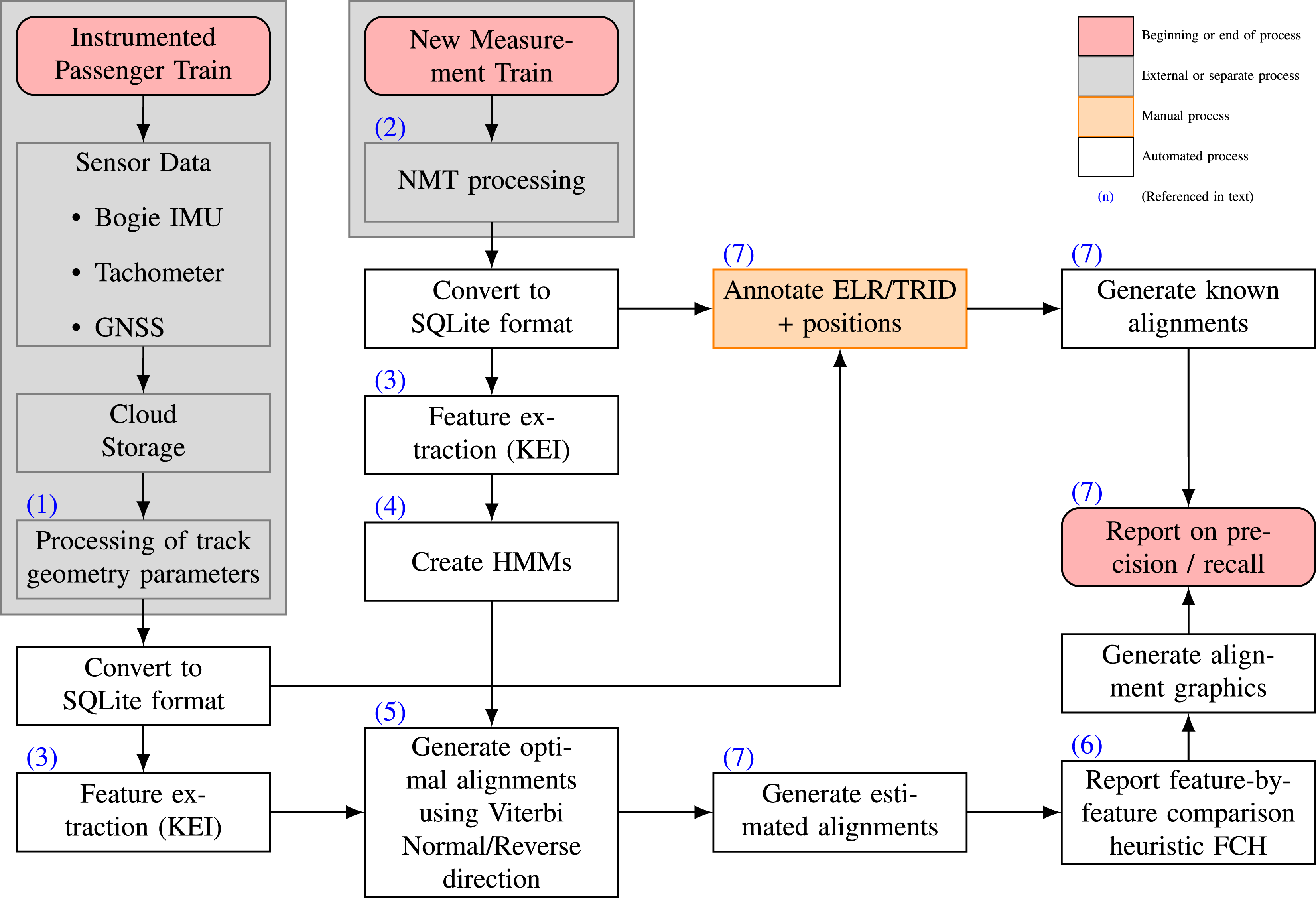
Track geometry processing
Raw time-domain data collected from IMU sensors is processed to extract track geometry estimates at 0.125 m intervals.7,16
NMT processing
Data recorded using sensors on the NMT is processed to extract track geometry estimates at 0.20 m intervals.3,32
Feature extraction
Each sample and reference recording is processed to identify a sequence of features, which is used as the basis for the reference HMMs and for the matching of sample recordings to reference recordings. 29
HMM formulation
Features extracted from each reference recording form the underlying state sequence of their corresponding categorical HMM. Each feature corresponds to a specific state, identified by its category (positive or negative lateral curvature). 42
Each categorical HMM is initialized with an m length initial probability vector P0 and m ⋅ m state transition matrix • probability of starting in the first state is 0.9 • probability of starting in any remaining state is uniformly distributed across the remaining probability
• probability of transitioning to the next state is 0.8 • probability of remaining in the same state is 0.1 • probability of transitioning to any future state after the next state is uniformly distributed across the remaining probability • probability of transitioning to any prior state is 0.0
For example, a five-state sequence would have the following P0 and
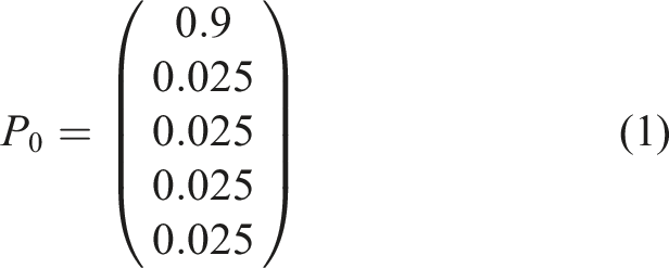
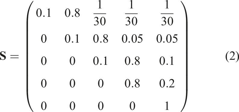
P0 and
Optimal alignment
Each sequence of sample features is divided into subsequences of length m, where m is the number of states in a given reference HMM. Each journey can be aligned to any number of reference HMMs. For an n length sample recording and an m length reference HMM of m features there are n − m − 1 possible subsequences. Furthermore, a track section can be traversed by the vehicle in either direction, so alignments are performed to both a normal and reversed set of features. The maximal-likelihood sequence of states traversed to give each m length subsequence of observations is found using the Viterbi algorithm. 42
The m length subsequence of features having the highest log-probability for a journey is annotated as the optimal alignment, indicating high likelihood of the order of states given observed sample features. The highest probability is for transition to the next state. Same-state and skipped-state probabilities are intended to handle missed features in the reference dataset or vice versa. Figure 3 illustrates this with an example. Robustness of HMM alignment algorithm to false negatives: State two is skipped as corresponding feature was not identified in sample.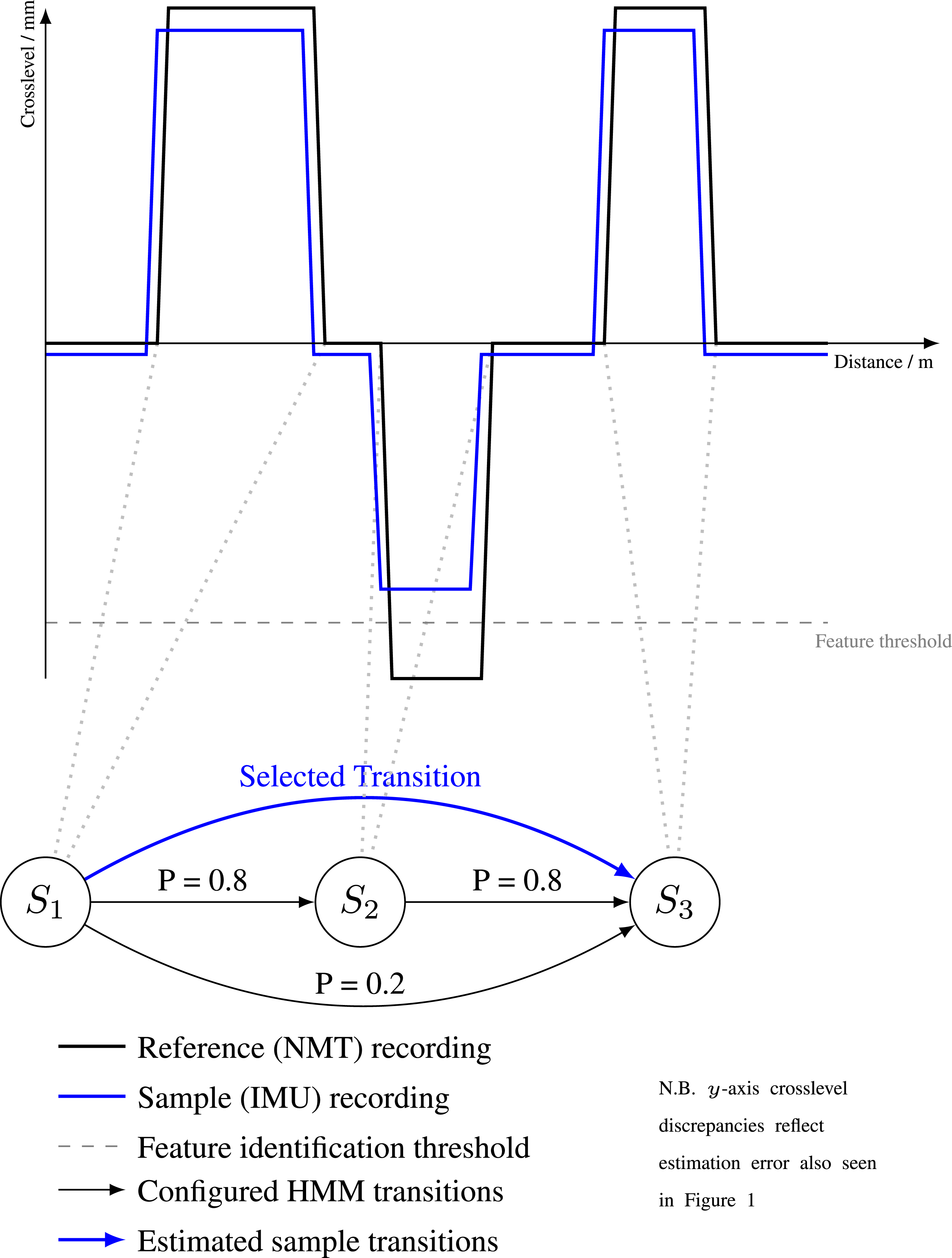
Identifying correct matches while rejecting false positives is challenging. Analysis in this paper assumes that the subsequence with the highest log-probability is a correct match to the reference. This assumption is reviewed in the conclusions.
Feature comparison heuristic
Each N length sequence of sample features is compared on a feature-by-feature basis with the N length sequence of reference features forming the HMM. This produces a statistic indicating similarity of sample features to corresponding reference features, denoted as Feature Comparison Heuristic (FCH).
On both a per-feature and per-sequence basis, FCH accounts for: • Variation in feature length between sample and reference • Variation in feature crosslevel magnitude between sample and reference • Proportion of overlap of sample feature with previous feature
FCH starts from 0, which indicates that two corresponding features are of equal length, equal crosslevel magnitude, and sample feature does not overlap with the previous feature. To summarize the overall similarity of an alignment to its reference, values of FCH for all sample features are summed.
A simple overlap correction algorithm applies a correction to the start x value of subsequent features if an overlap is found for every alignment produced by HMM-AA.
Alignment validation
HMM-AA produces N ⋅ M optimal alignments, where N is the number of sample recording journeys and M is the number of reference recording journeys. Two methods are used to validate HMM-AA, both of which rely on annotation of expected track sections.
Expected track sections
Each of the N sample recordings has 0–M expected track sections. These are annotated by hand following extraction of features from IMU journey recordings, and indicate: (a) Discrete track sections (ELR/TRID codes) are traversed by the journey (b) Order in which specific track sections are traversed (c) For each track section traversed, x values within sample recording where traversal of specific section starts and ends
Validation using FCH
Each N ⋅ M optimal alignment has a corresponding FCH value. The optimal value of FCH is found across all alignments which maximizes retrieval of relevant (i.e. correctly identified) alignments.
Precision, recall and F1 statistics can be computed for any threshold of FCH. These statistics are used in classification and information retrieval problems, though have limitations in their ability to assess algorithm performance. 43 The optimal value of FCH is the value for which maximal values of precision, recall and F1 are obtained.
In this study, each sample recording could be matched to 0–M reference recordings, therefore the contribution of each recording to the overall values of precision and recall (i.e. number of retrieved, relevant, and relevant retrieved instances) may be more than 1. This is accounted for in formulation of the total for each instance.
Validation using location overlap
Each N ⋅ M optimal alignment having a corresponding expected track section is selected. For each optimal alignment, the following values can be found: • Expected x values in sample recording corresponding to start and end of specific track section, based on the annotated expected track section • Estimated x values from optimal alignment of sample features to reference HMM, based on x values of start feature and end feature • Proportion of overlap of estimated track section with expected, indicating whether HMM-AA derived alignment fits entirely or partially within expected range
These values are used to summarize the proportion of optimal alignments fitting entirely within the expected range, indicating that the correct subsequence of sample features was selected.
Case study
The HS1 line from London St Pancras to Folkestone in Kent, UK was selected as the case study. This is the only high-speed line currently in operation in the UK, chosen due to its simple geography of two lines (an Up line, towards London from Folkestone, and a Down line, towards Folkestone from London) and minimal switches & crossings. This reduced the number of possible track sections that could be matched as all journeys fit into the categories outlined in Figure 4. Recording data was available from a Eurostar Class 374 train instrumented with a IMU covering the period from 12-Nov-2022 until 27-Dec-2022 (45 days). The line is split into three track sections by ELR code, with NMT recording data available for two: HS1 (North) and HS1 (South) in Figure 4. NMT data covering 11 dates between 27-Aug-2021 and 21-Oct-2022 was available, however only the first recording contained crosslevel data. Track geometry recordings and Track Sections: (a) North and South sections of HS1, (b) full Down line, (c) full Up line.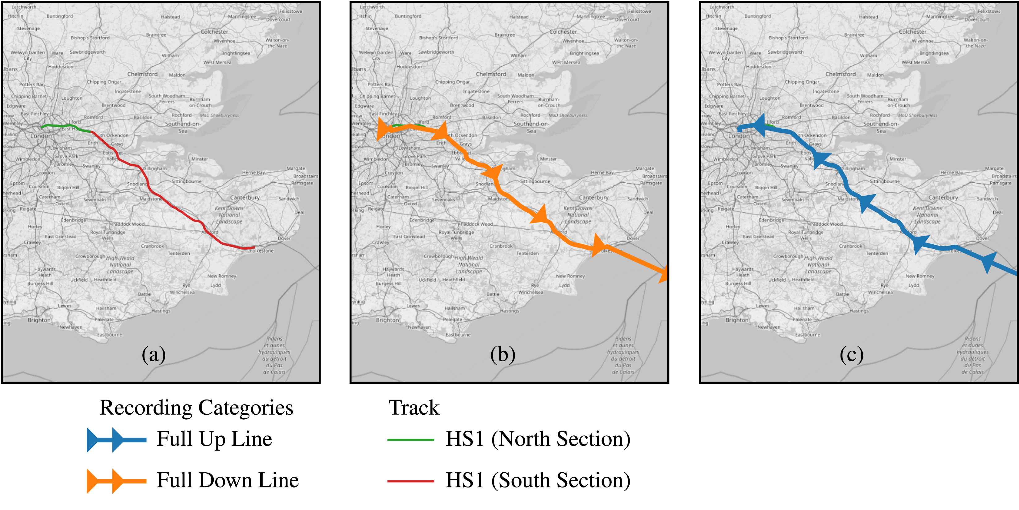
While data was recorded both inside and outside of the UK, this study was concerned solely with alignment to track sections situated within the UK.
Results and discussion
An example of unaligned and aligned recording data can be seen in Figure 1. Figure 5 and Table 1 summarize the results of this case study. Summary graphics from HS1 case study: (a) Precision, Recall and F1 Curves, (b) Correctly versus Incorrectly Matched Sections, (c) Amount of Overlap with Expected Track Sections. Summary of validation results for HMM-AA in this case study.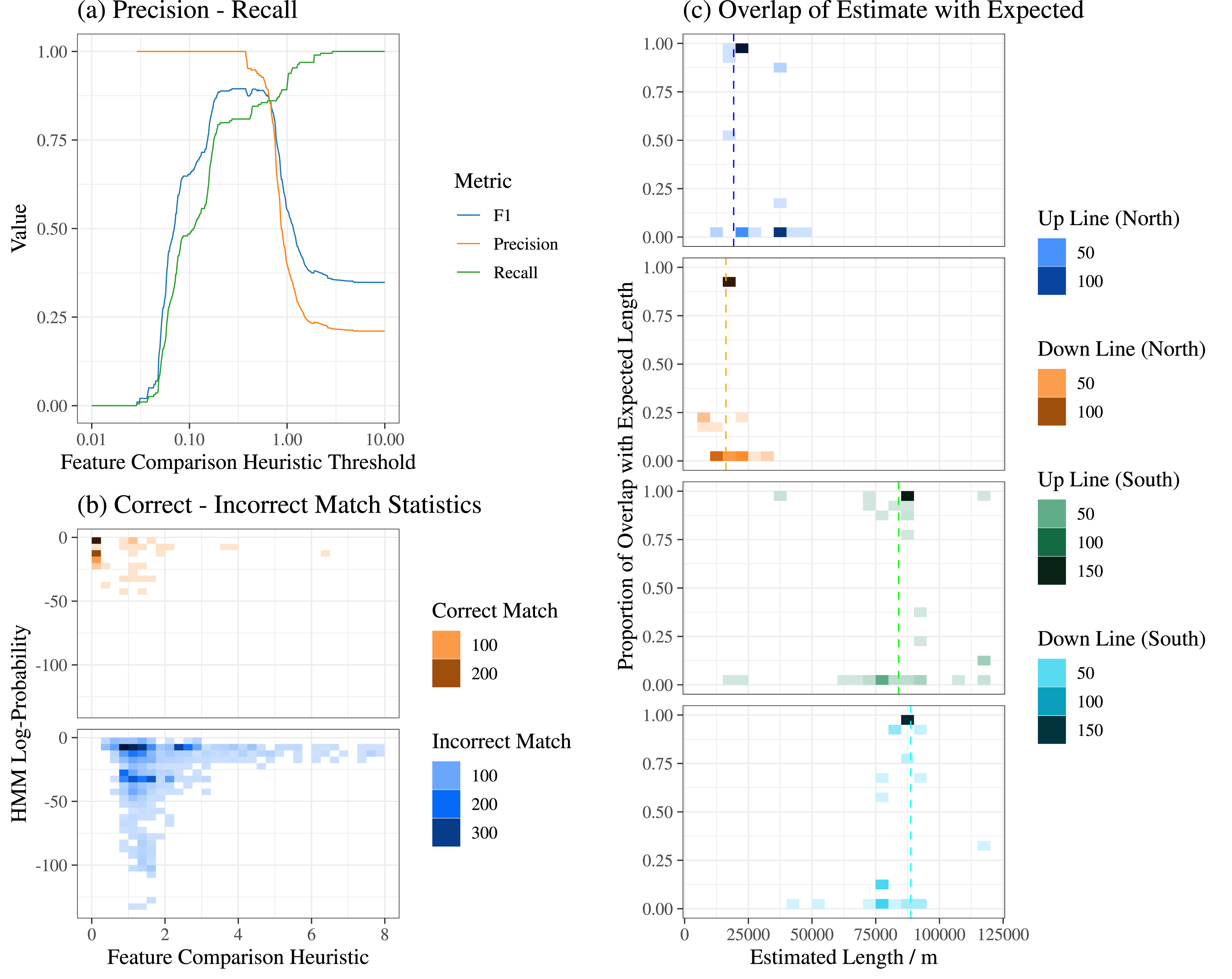
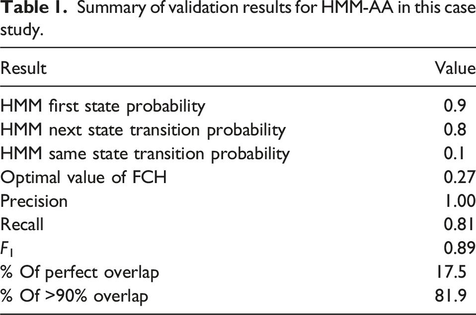
Figure 5 presents three graphics. Plot (a) presents variation of precision, recall and F1 (see page 5) with different thresholds for feature comparison heuristic FCH. The highest value of F1, 0.89, is found at FCH = 0.27 with corresponding precision of 1.00 and recall of 0.81. These values are presented in Table 1.
Plot (b) presents two 2D-histograms. The density variable (darkening gradient) is the number of optimal alignments. One journey may have up to 16 optimal alignments: 4 track sections, two directions (normal or reverse) and two feature configurations: unshifted or shifted (see page 5). The two panels and color schemes indicate whether the optimal alignment corresponds to the expected track section (see page 5): correct matches indicated with orange gradient, incorrect matches with blue, and darker shading indicates higher density of alignments in that quadrant. The two independent variables shown are HMM log-probability (x -axis) and FCH (y -axis) for the optimal alignment in question. Quadrants to the left indicate close similarity between sequences of features in the sample and reference recording. Quadrants to the top indicate a high probability of the feature sequence being observed in the HMM. For example, the top-left quadrant indicates high similarity between sample and reference features along with high likelihood of that specific sequence of sample features being observed given the corresponding HMM.
Plot (c) presents four 2D-histograms. The density variable (darkening gradient) is the number of optimal alignments matching the expected track section. The four panels and color schemes indicate which track section the alignment was matched to. There are four track sections (two on the Up line, two on the Down line) making up the section of line studied (see Nomenclature on page 9 for detail on the North and South sections). The x axis displays the estimated length of track (i.e. the distance between the estimated start and end features obtained from the Viterbi algorithm). The y axis displays proportion of overlap with the expected track section: 1 indicates that estimated length fits entirely within expected length, and 0 indicates that estimated length is entirely outside expected length. A dashed vertical line indicates mean expected length of track for given track section across all optimal alignments for that track section. Darker shading indicates a higher density of alignments in that quadrant. Quadrants to the top indicate that selected sample track segments are coincident with selected reference HMMs, indicating good performance. Conversely, quadrants to the bottom indicate that track segments were selected that are not near to the reference, indicating poor performance. The North section of HS1 is 60 km shorter than the South section, shown by differing positions of the dashed vertical line. Quadrants around this line on the x axis indicate that selected sample track segments have similar length to mean expected reference length; this generally indicates good performance, though expected length does vary between recordings due to differing start and end locations.
Out of all optimal alignments, 17.5% fit entirely within expected lengths (‘perfect’ overlap), corresponding to values of 1.0 in Plot (c); 81.9% of optimal alignments overlapped by more than 90% with their expected lengths, corresponding to values of 0.9 or higher in Plot (c). These values are presented in Table 1 along with the parameters used for configuring the HMM.
Discussion
Plot (a) shows that actions increasing precision result in decreased recall, typical in classification problems. The value of FCH maximizing both precision and recall, 0.27, results in precision of 1.00 indicating all selected optimal alignments at this threshold are matched with the expected track section. This demonstrates that global alignment from recordings to traversed track sections can be found without additional sources of position data, and that a threshold can be selected resulting in no false positives.
Plot (b) allows further understanding of the precision-recall graph. Optimal alignments matched to correct track sections (orange) are clustered in the top-left with values of FCH <0.25 having high density. There are no incorrectly matched optimal alignments (blue) with values of FCH <0.25. Incorrect matches show wider distribution of both FCH and log-probability. However, large magnitudes of both FCH and log-probability are seen even for optimal alignments expected to produce a match. High values of FCH indicate HMM-AA picking a subsequence of features providing a good match to the HMM but poorly aligned when compared feature-by-feature. Large negative values of log-probability indicate that the maximally likelihood sequence of features has a low certainty. This is seen for longer recordings which tend to have lower values of FCH and higher values of log-probability, indicating difficulties in identifying matches based solely on log-probability. Alignments matched to TRL2 have lower log-probability and higher values of FCH from having fewer features, comprising a high proportion of the ‘tail’ observed in the incorrect match graphic.
Plot (c) shows two distinct categories of alignments: those matching with overlap of >75%, and those not matching with overlap around 0%. The highest density of alignments are all ≈100% and, for all four track sections, these alignments all had estimated lengths around the mean expected value (vertical line). The global nature of HMM-AA provides an explanation: an alignment could occur from any subsequence of features in the recording and the matched section could be far from the expected section. Longer track sections (TRL3) have higher variation in estimated track length from having more features than shorter sections (TRL2), leading to high range in distances between features.
Conclusions and future work
HMM-AA, introduced in this work, demonstrates general-case alignment of track geometry recordings taken from in-service vehicles enabling autonomous comparison of track monitoring recordings at scale without manual input. HMM-AA aligns recordings using track geometry features (curves, switches & crossings) to HMMs trained on TRV recordings, reducing the mean number of data points involved in producing an alignment from ≈ 900000 sample points to ≈100 features following feature extraction.
Precision and recall metrics were generated for different thresholds of FCH with a value of 0.27 found to be optimal for this study, giving an overall precision of 100% and recall of 81%. Each estimated track section was compared with pre-annotated expected locations to confirm the correct section was selected. 17.5% of recordings fully overlapped with expected locations, with 81.9% overlapping with over 90% of expected range. Over 80% of possible alignments were false positives, excluded through FCH which heavily penalized remaining in the same state. Other improvements to global matching accuracy are suggested later in this section.
This implementation of HMM-AA took 127 minutes to calculate 9576 combinations of optimal alignments. An average track section length of 50 km gives a mean solution time of 15 ms per km. DTW, by contrast, takes around 1.5s per km. 27 Local and global alignment algorithms cannot be reliably compared in this way, and DTW can complement HMM-AA to provide higher quality local alignment.
This study included 45 journeys which traversed the entire Up line and 49 journeys which traversed the entire Down line, over a period of 45 days. With 75% of these journeys successfully matched with correct track sections, a mean monitoring period of 32 hours can be achieved. While there were extended periods in which the specific instrumented vehicle was not in service, instrumenting additional vehicles in operation along the route would further increase the frequency of track monitoring on the HS1 line. It is, therefore, not necessary to achieve 100% recall in matching of recordings in order to monitor changes in track geometry condition and success rates presented here are sufficient to provide frequent assessment of both running lines, augmenting regular TRV-based inspection. It is possible to improve this further, enabling greater network coverage from in-service railway track condition monitoring, as outlined below.
Future work
Extraction and storage of track features can be implemented alongside track geometry data acquisition as a standard process. This could be done in the time-domain, allowing alignment to be performed immediately after data acquisition and with minimal computational overhead. Further work could use additional information to constrain journeys investigated e.g. infrastructure constraints (line speed, line direction), geofencing (location of recordings), planned timetable and actual routing of the instrumented train service, to form the topic of future work by the author in this area.
The ‘uncertainty’ of a given journey, defined as spatial difference between corresponding distances on sample and reference at end of reference recording following alignment to start of reference, merits investigation. A non-zero value for uncertainty indicates systematic errors in estimation of speed and distance in sample recordings or errors in reported distances in reference recordings, and could be investigated further using the ‘uncertainty’ metric in an optimization model. The impact of uncertainty on estimation of track geometry parameters, given position estimation and track geometry estimation are sensitive to speed, is not understood and quantified, and providing robust analysis of error bounding in track geometry estimation may assist business adoption of this technology.
Further improvements to HMM-AA would include biasing the algorithm against selecting significantly different length sample track sections to the reference to address the horizontal drift seen in Figure 5(c), investigation of sensitivity of generated alignments to HMM parameters, alerting to misidentified or duplicated features through inclusion of feature magnitude and width, and improving crosslevel estimates using a regression model.
HMM-AA was not designed to automatically identify misidentified or duplicated features. Through further analysis of FCH and comparison of feature magnitudes and widths, corresponding features having different feature widths could be identified and combined with a regression model for improving crosslevel estimates based on statistical differences with reference data.
The key issue causing misalignment of datasets is error and uncertainty introduced with speed, distance and position estimation. This has further impact on track geometry estimation as track geometry value estimation from inertial sensors is highly dependent on speed. The methodology presented here enables future work on quantification of distance and speed estimation errors and their impact on track geometry estimates.
This study purposefully selected a line of route with minimal switches & crossings to demonstrate the principle of the algorithm. For journeys through more complex geography, introducing constraints on vehicle position would reduce the search space size for alignment and improve confidence in alignment quality. Further work is needed to validate FCH in such geography alongside integration with geospatial positioning methods. Finally, business challenges in managing adoption of in-service condition monitoring will present themselves in future development of this technology.
Widespread instrumentation of in-service vehicles will lead to significant volumes of monitoring data which can be used to monitor degradation of railway track geometry. The techniques introduced in this paper enable the utilization of this data to provide insights on developing faults at a daily or even hourly frequency compared with a monthly frequency from TRVs, enabling a data-driven approach to preventive maintenance and reducing the risk of line closure and disruption to passengers and freight customers.
Footnotes
Acknowledgements
The authors acknowledge MoniRail, Network Rail High Speed, Eurostar Engineering Centre and Eurotunnel for supporting this work. Map data from OpenStreetMap.
Funding
The authors received no financial support for the research, authorship, and/or publication of this article.
Declaration of conflicting interests
The authors declared no potential conflicts of interest with respect to the research, authorship, and/or publication of this article.