Sage Journals: Discover world-class research

Abstract

This study investigates numerically the effects of bogie side component positions on the flow behaviour and aerodynamic noise of high-speed trains. To reduce simulation cost, the model size and flow speed are scaled down, while ensuring that the Reynolds number remains within a range conducive to similar flow behaviour. The Delayed Detached Eddy Simulation method with Spalart-Allmaras turbulence model is adopted for flow simulations. The time histories of the wall pressures are employed to predict the far field noise using the Ffowcs Williams and Hawkings equation. Analysis of pressure fluctuations on the bogie and car body show that, as the bogie side components protrude further into the flow, the area exhibiting strong noise source on the bogie surfaces increases, while it decreases on the rear walls of the bogie cavity. The aeroacoustic results reveal that the radiated noise rises at higher frequencies and drops below 160 Hz for the bogie and 300 Hz for the car body as the side components protrude further. When the bogie side components are shifted outwards by 400 mm, the overall unweighted sound pressure reduces by 2 dB but the A-weighted level increases by 2.5 dB. The total A-weighted sound power level is increased by 2.9 dB compared to the reference case.

Keywords

Train bogie aerodynamic noise side components DDES Ffowcs Williams & Hawkings

Introduction

At speeds above 300 km/h, the noise produced by high-speed trains increases more rapidly due to the presence of aerodynamic noise.¹ There are various aerodynamic noise source regions on a high-speed train, such as the bogies, pantographs, gaps between coaches, train nose and the wake region.^2–7 Of these, the bogie regions have the largest contribution to the overall sound power.⁴ Among the various components of the bogie, those on the sides significantly impact the noise generation due to their proximity to high-speed flow outside the bogie cavity.^5,8 These side components include the axleboxes, the bogie side frames, and external suspension dampers. In reality, their lateral location relative to the car body can vary between different designs of vehicle due to differences in the train loading gauge and the track gauge. These differences are expected to affect the aerodynamic noise from the bogie region. Therefore, it is of great practical significance to study how the lateral position of the bogie side components influences the noise generation from the bogie region.

Latorre Iglesias et al.⁵ investigated the aerodynamic noise generated by a 1/7 scaled bogie model in a wind tunnel. The effect of the lateral positions of bogie side components was investigated by extending one side of the bogie laterally by up to 100 mm, thereby exposing the side components to the incoming flow. Increased noise levels were observed as the bogie side frame protruded further from the cavity, which were mainly attributed to intensified pressure fluctuations due to greater exposure of certain bogie components to the incoming flow. However, the mechanisms behind these changes were not thoroughly analysed due to the limitations of experimental methods.

As well as experimental studies, various numerical investigations of bogie aerodynamic noise have been carried out. Zhu et al.³ investigated the effect of a fairing on bogie noise in a simplified cavity using delayed detached eddy simulations (DDES) for flow and the Ffowcs Williams and Hawkings (FW-H) equation for far-field noise. The fairing installed at the side of the bogie cavity reduced pressure fluctuations by preventing upstream flow from interacting with bogie components, leading to a significant reduction in aerodynamic noise. This suggests that noise generation around the bogie region is greatly influenced by the flow conditions at the sides of the bogie cavity. He et al.^8–10 used similar methods with a more detailed bogie model, which included additional components. They further extended the study by incorporating the bogie into a realistic car body. Strong noise sources were identified at the rear wall of the cavity, the bottom of the bogie and on the side components such as dampers, axle boxes and wheels, which is caused by impingement from the detached shear layer at the cavity’s front edges. This finding agrees with results from Minelli et al.,¹¹ who identified the shear layer detached from the surface of the car body as the primary cause of noise sources on the bogie.

Both previous experimental and numerical studies suggest that bogie aerodynamic noise is closely related to the positions of side components relative to the upstream shear layer. The aim of this study is to use numerical methods to examine the mechanism behind changes in noise spectra and overall sound pressure levels when side components extend outside the bogie cavity. Detailed simulations investigate flow parameters and noise for various configurations with different lateral positions of bogie side components. The flow field is calculated using the DDES method, and far-field noise is assessed via the FW-H equation. Flow features, noise source distributions, sound pressure levels (SPL), and sound power levels (SWL) of different components are analysed and discussed.

Computational setup

Computational model

The flow along the sides of the bogie cavity influences the noise from the bogie side components such as axleboxes, dampers, and air springs, while components positioned between the wheels like motors, gearboxes, or disc brakes are primarily affected by the flow entering the cavity from the bottom.¹⁰ Therefore, to minimize the computational expense, the components between the wheels are omitted from the computational model, as seen in Figure 1(a), rendering the bogie model symmetric. The local flow around the bogie side components is not significantly affected by the flow at the other side of the car body. In addition, the noise propagation in the turbulent flow around the car body will not be considered in the current study. Therefore, these conditions justify the use of a half-width model, with a symmetry plane introduced on the central plane of the vehicle.

Figure 1.

Computational model and its dimensions; (a) the bogie model; (b) the side view of the model; (c) the computational domain (half-width model).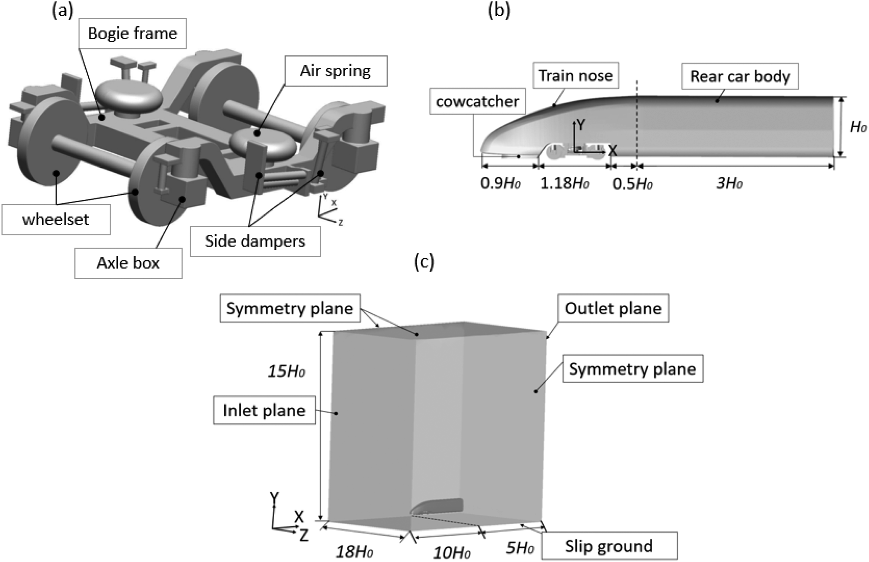

Figure 1(b) and (c) show the dimensions of the computational domain, which are scaled with respect to the height of the train body H₀ (3.795 m at full scale). For convenience, the train coordinates are chosen, in which the train is stationary, while the incident flow moves in the opposite direction at the train’s operating speed. Fixed velocity boundary conditions are assigned at the inlet plane and a zero-pressure outlet boundary condition is specified at the outlet plane. The top, middle and side planes are assigned symmetry boundary conditions. The positions of the upstream boundary and the various symmetry boundaries were carefully chosen to be far enough away to avoid any impact on the flow around the vehicle. All solid surfaces of the train are set as non-slip walls.

The length of the train model is approximately 5.6H₀. The inlet plane is located around 10H₀ away from the train nose. This distance is carefully chosen according to the numerical study in Minelli et al.,¹¹ Li et al.¹² and Wang et al.¹³ To minimise the influence from the outlet boundary condition at the downstream end, while restricting the size of the model, the first carriage is truncated at a position 3.5H₀ behind the rear wall of the bogie cavity, just before the location of the second bogie cavity. According to the research from Minelli et al.,¹¹ Gao et al.¹⁴ and Zhang et al.¹⁵ a distance of 3.5H₀ is sufficient to allow a zero pressure boundary condition to be specified at the outlet plane. Since the focus of this paper is on the area of the bogie side components, the rails have been omitted for simplicity; the ground is located at a nominal distance of 250 mm below the bottom of the wheels. The moving ground effect is not considered, and thus, a slip wall boundary condition is assigned to the ground.

The position of the side components of the bogie relative to the car body varies with different combinations of train loading gauge and track gauge. Different widths of the car body are required for compatibility with different train loading gauges. However, for convenience, the shape of the car body is kept unchanged in the simulation (the width of the car body W = 3.444 m in full scale) and the lateral position of the bogie components is varied by extending the wheelset axles and other transverse members, similar to the approach used in the experiments of Latorre Iglesias et al.⁵

In addition to standard gauge track (1435 mm), various broad gauges are used (ranging from 1524 mm to 1610 mm) as well as narrow gauges (1067 mm or smaller). The loading gauge varies according to the age and design of each country’s railway system. Across various loading gauges, the width of the carriage ranges from 2.7 m to 3.4 m. Based on these combinations of loading and track gauges, four cases are considered. As shown in Figure 2. In the case m100, the axles are shortened by 100 mm (full scale) on each side, resulting in more components being shielded by the cavity compared to the reference case. In cases 200 and 400 the wheels are shifted outwards by 200 mm and 400 mm (full scale) on each side. These two cases represent generically a smaller loading gauge (such as that present in the UK) and standard track gauge. In these two cases, more side components of the bogie will protrude from the side of the cavity, leading to an expected acceleration of the flow impacting those components.

Figure 2.

Sketch showing the relative positions of the bogie components with respect to the car body for the different wheelset axle extensions: −100, 0 (reference), 200 and 400 mm (at full scale on each side). End view with vertical direction towards the left of the figure.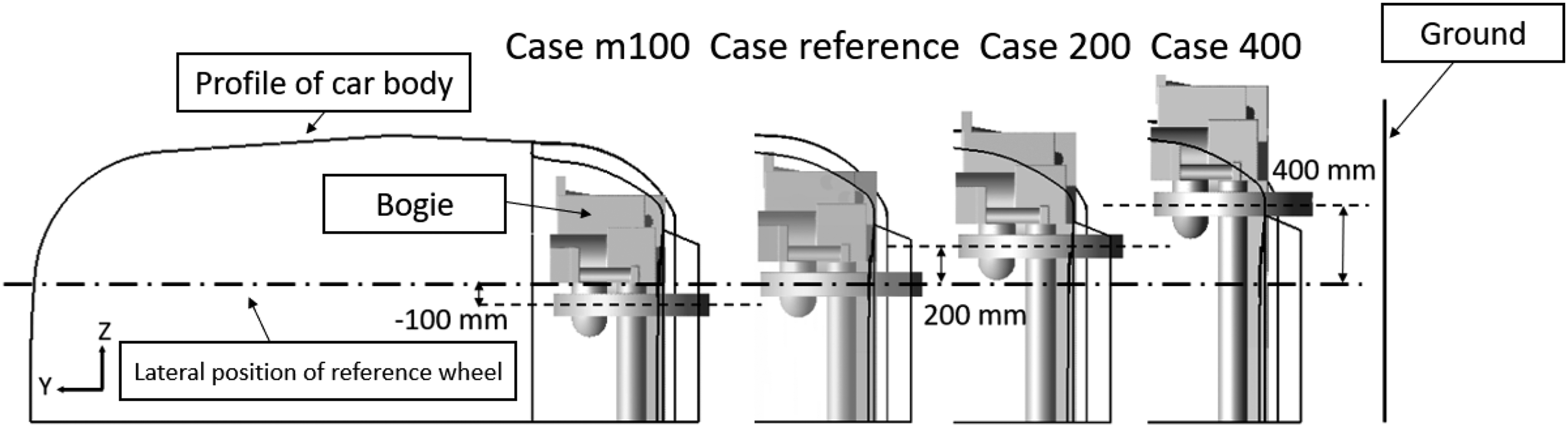

Grid strategy and numerical set-up

The primary challenge in aeroacoustic calculations of the bogie is to obtain acceptable simulations of the complex flow.⁴ The complicated geometry and flow phenomena around the bogie make achieving a suitable discretization of the computational domain extremely challenging. This involves maintaining good grid quality while limiting the number of cells within acceptable bounds, especially within the boundary layer regions on solid surfaces where large velocity gradients occur. The boundary layer plays a crucial role in influencing flow transition, separation, and vortex generation. Moreover, the complex flow phenomena around the bogie, driven by the high Reynolds numbers and complex geometry, necessitate a fine grid resolution, leading to very high computational costs.

To reduce the computational cost, which would otherwise be impractical, the model’s geometrical size is scaled down to 1/12 of full scale, and the operating speed is reduced to 10 m/s, approximately 1/11 of the full-scale speed (400 km/h). The Reynolds number of the scale model is ${1.91 \times 10}^{5}$ , based on the scaled width of the car body (0.287 m), which remains greater than the minimum Reynolds number ( ${1.53 \times 10}^{5}$ ) tested by Lauterbach et al.¹⁶ The study from Lauterbach et al.¹⁶ revealed that, within the Reynolds number range they investigated ( ${1.53 \times 10}^{5} \sim {3.7 \times 10}^{6}$ ), the sound power levels and spectral shapes did not change significantly, after applying suitable scaling in magnitude and frequency. Thus, the noise behaviour of the first bogie was largely independent of Reynolds number within this range. The speed exponent was found to be close to 6, indicative of typical dipole noise sources. To confirm the validity of the Reynolds number chosen for the present study, preliminary calculations were performed on a simplified model, which included a bogie in a simplified cavity. These calculations were performed for two values of Reynolds number ( ${1.91 \times 10}^{5}, {6.9 \times 10}^{6}$ ) using a coarse mesh. The results showed similar flow direction, vortex structure, and spectra of drag and lift coefficients up to 1000 Hz (at full scale). Surface pressure spectra on the bogie surface at monitor positions were also found to be similar, confirming that essential flow features are retained in the reduced scale model, and justifying the use of the smaller Reynolds number. Additionally, the numerical study by Qin et al.¹⁷ demonstrates that simultaneously scaling down the model size and reducing the flow speed can preserve the overall shape of the noise spectra when extrapolated back to the full-scale model. He¹⁸ also discussed the validity of using reduced model size and speed and the potential impact on noise simulation accuracy.

To discretize the complex geometry in Figure 1, a hybrid grid system is adopted that was previously explored by He.¹⁸ The efficiency of the hybrid grid has been validated through the basic geometrical elements, such as circular cylinder, square cylinder and an isolated wheel. The aerodynamic and aeroacoustic results show that the hybrid grid has as good a performance as the hexahedral grid. The detailed information about this type of grid is available in studies by He et al.^8–10,18 Figure 3 depicts the grid distribution of the model. The origin of the coordinates coincides with the symmetry plane in the current half-width model.

Figure 3.

Grid distibution of the model: (a) surface mesh on simplified bogie; (b) surface mesh on leading car body (front part); (c) horizontal slice through the centre of the air spring at Y = 522 mm (full scale); and (d) vertical slice through the wheels at Z = 768 mm (full scale).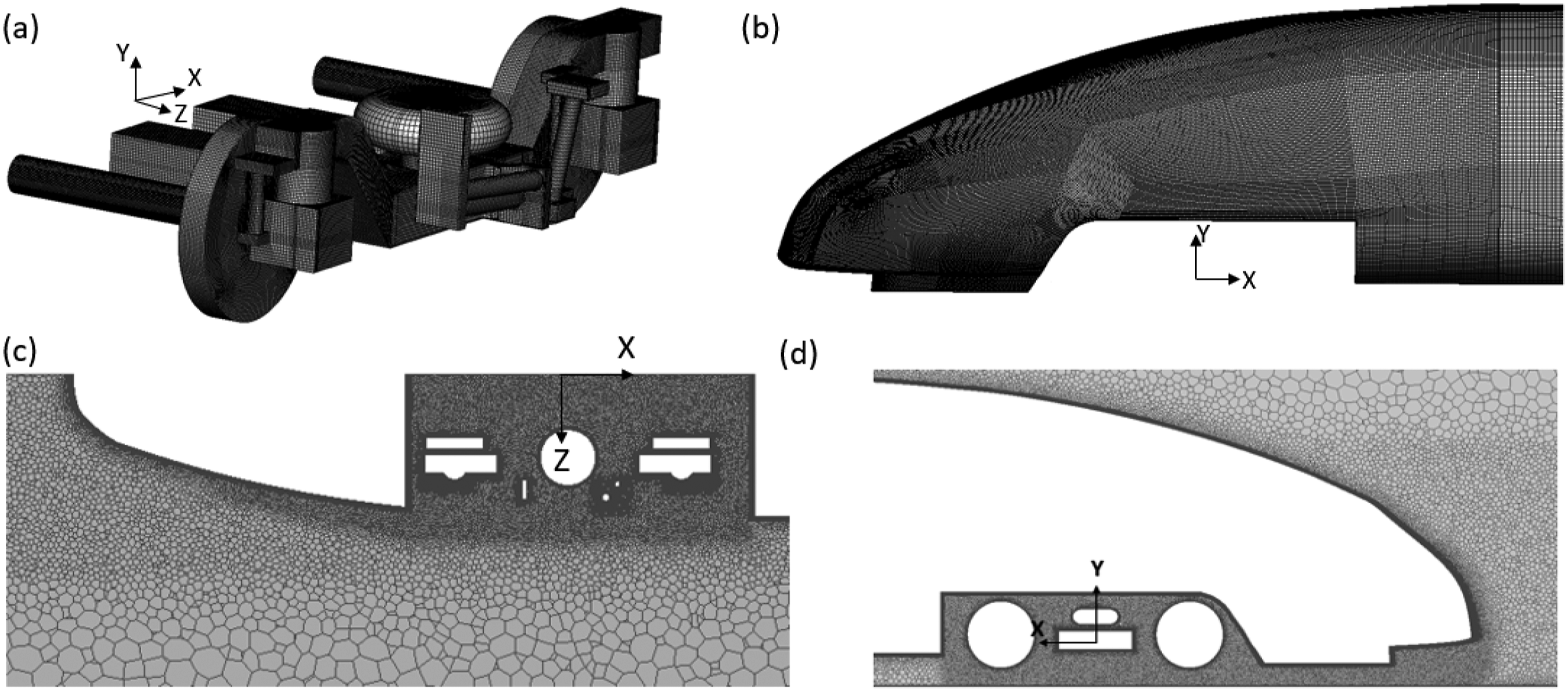

The grid parameters, e.g. the height of the first cell close to the solid surface and its maximum aspect ratio, are based on a comprehensive mesh sensitivity study by He et al.^8–10,18 The parameters of the boundary layer grid match those utilized in the study conducted by He et al.¹⁰ The value of non-dimensional cell size y + on the solid surface is less than 1, meeting the requirement of the Delayed Detached Eddy Simulation with Spalart-Allmaras turbulence model. The aspect ratio of the first cell in the boundary layer is the ratio of the longest edge parallel to the wall to the cell height. The maximum aspect ratios of the bogie components range from 65 to 128, while those of the car body range from 115 to 220. Particular attention was paid to the grid refinement in the train nose and bogie cavity regions. As seen in Figure 3(c) and (d), the grid near the regions of the train nose and bogie cavity was particularly refined. The refinement cell size is 2.0 mm at reduced scale. The total cell count for each case considered here is around 13.9 million.

The flow simulation was conducted using OpenFOAM v2.4.0. The Delayed Detached Eddy Simulation with Spalart-Allmaras turbulence model is adopted. The application of this numerical method has been validated in references 8-10 and 18 . A steady Reynolds-averaged Navier Stokes (RANS) calculation preceded the unsteady DDES simulation to initialize the flow field.

A physical time step of $2.2 \times 10^{- 5} s$ was used, which ensures that the Courant-Friedrichs-Lewy (CFL) number remains smaller than 5. This time step was carefully chosen by a convergence study. Detailed information on the timestep study is available in reference 18. The CFL is defined as $U ∆ t / ∆ x$ , where $∆ t$ is the time step size, $∆ x$ is the smallest cell size in the X direction and $U$ is the local velocity. The maximum CFL value appears at the gap between the downstream wheel and the axlebox, where the grid is very fine, whereas for other regions, the CFL is below 2.

Simulations for the four cases indicated in Figure 2 were run for a minimum duration of 4.5 s, corresponding to 125 flow-through times of the bogie cavity length. The data collection commenced after 0.6 s, when the simulation had become statistically steady. The computational wall-time was approximately 240 hours, utilizing 480 processors on the Iridis5 HPC at the University of Southampton.

Aerodynamic results

Flow field

The analysis of the flow field is conducted in the scaled condition. Figure 4 displays the streamwise velocity field for all four cases, along with two-dimensional streamlines on a horizontal plane at Y = 200.9 mm (full scale), which passes through the axis of the wheels and the axles. Figure 5 shows the corresponding instantaneous vertical vorticity (ω_y) fields, visualizing regions of strong vortical motion in the flow. Towards the outside of the bogie, the regions with high negative values (blue colour) represent the shear layer detached from the surface of the car body. For case m100 and the reference case, presented in Figure 4(a) and (b) and in Figure 5(a) and (b), the side components are almost completely shielded by the bogie cavity from the high-speed air flow. Meanwhile, the outer part of the rear wall of the cavity is exposed to the detached shear layer originating from upstream. However, as the lateral extension of the side frame increases, for cases 200 and 400 shown in Figure 4(c) and (d) and in Figure 5(c) and (d), some of the side components protrude out of the cavity and become exposed to the external high speed flow. Consequently, the protruding side components deflect the high-speed flow away from the rear corner of the cavity wall, as indicated by the red arrows. The differences in the flow field are primarily caused by changes in the position of the bogie side components. When the side components are shielded by the cavity, the detached shear layer from the front edge bypasses them and impinges on the rear wall. However, when the side components protrude further, they shield the rear wall, preventing it from directly facing the shear layer.

Figure 4.

Average streamwise velocity contours and streamlines of the four cases on a horizontal slice at Y = 209 mm (full scale). H₀ is the car body height; (a) Case m100; (b) Reference case; (c) Case 200; (d) Case 400.

Figure 5.

Instantaneous vorticity fields of the four cases, H₀ is the car body height; (a) Case m100; (b) Reference case; (c) Case 200; (d) Case 400.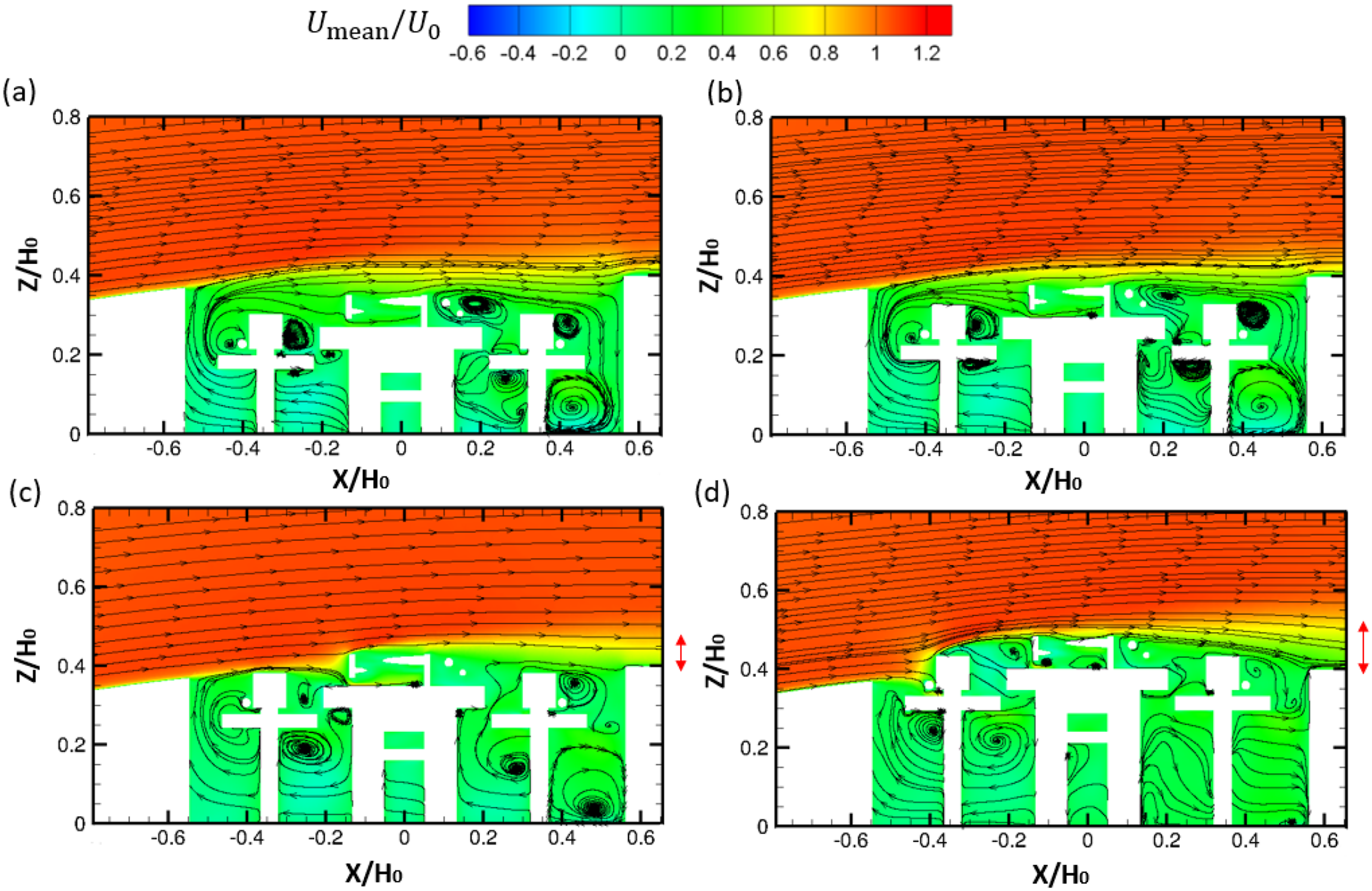

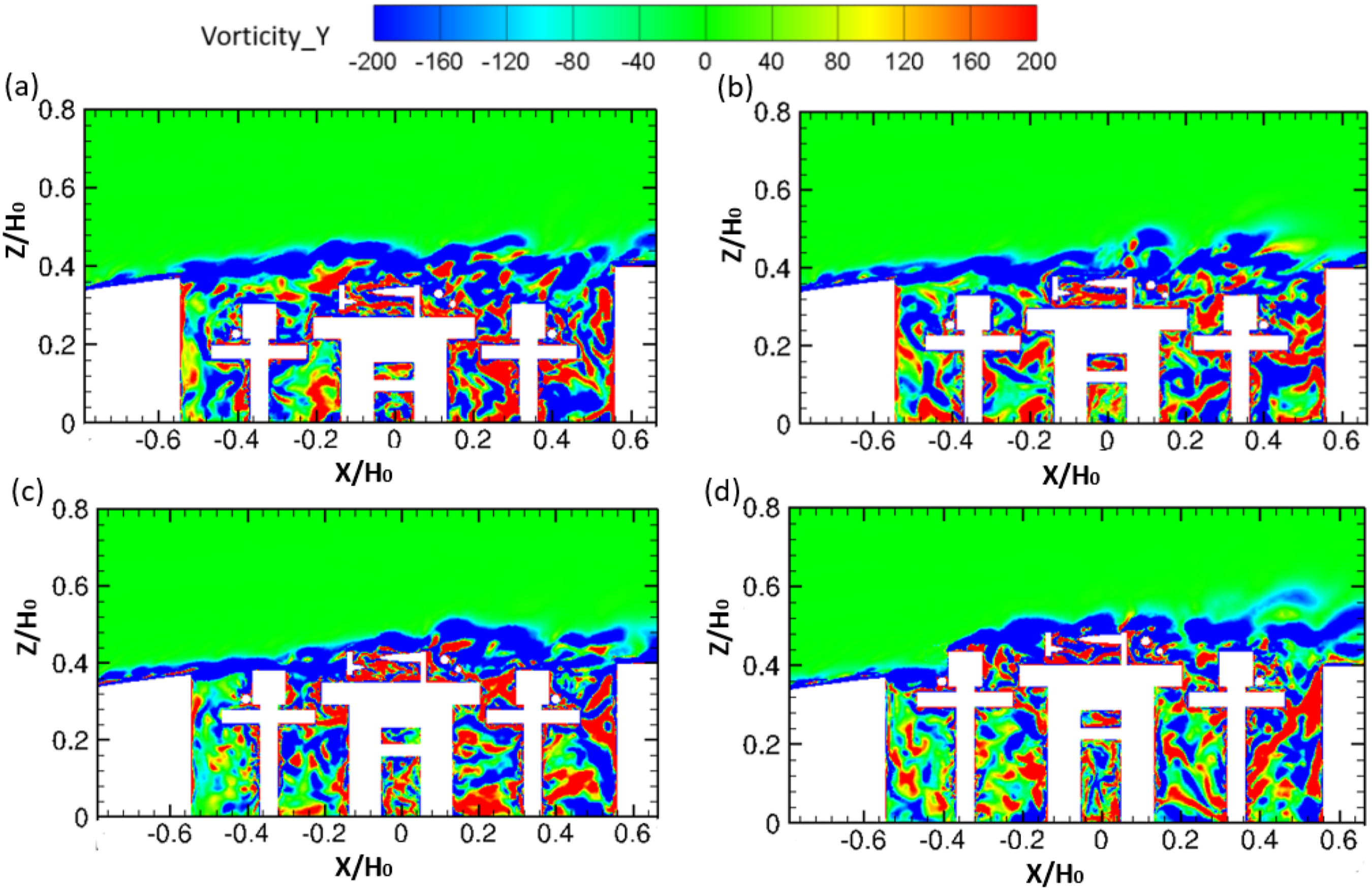
Figure 6 displays the vortex structure using iso-surfaces of $Q / {(U_{0} / H_{0})}^{2}$ at a value of 25, where $Q$ is second invariant of the velocity gradient, $U_{0}$ represents the free stream velocity and $H_{0}$ denotes the car body height. The iso-surfaces are coloured based on the normalized streamwise velocity $U / U_{0}$ . The observations from Figures 4 and 5 are confirmed by this 3D view. In Figure 6(a) and (b), the vorticity is initially formed by the shear layer at the front edge of the bogie cavity. However, Figure 6(d) clearly shows that the protruded components generate a significant turbulent wake. This is because the protruding side components obstruct the shear layer, causing detached flow to form around them. Nevertheless, this turbulent wake appears to be further from the cavity rear wall, which reduces the incoming flow speed compared to other cases, as shown in Figure 4(d). As seen in Figure 5, less of the turbulent wake impinges on the cavity rear wall compared to other cases, which is expected to reduce pressure fluctuations on it.

Figure 6.

Instantaneous vortex structures, represented by the Q-criterion at the side of the model for four cases; (a) Case m100; (b) Reference case; (c) Case 200; (d) Case 400.

Noise source strength

The rate of change of surface pressure dp/dt can serve as a valuable indicator of the noise source strength distribution on the solid surfaces, as according to Curle¹⁹ the fluctuation of dp/dt is related to the far-field sound pressure. In Figure 7, dp/dt is plotted in decibel form, $L_{\dot{p}} = 20 \log_{10} ({(d p / d t)}_{r m s})$ in dB re 1 Pa/s. The primary distinctions among the distributions of $L_{\dot{p}}$ for the four cases are seen on the side components, as well as the area around the rear of the cavity.

Figure 7.

Surface contours of 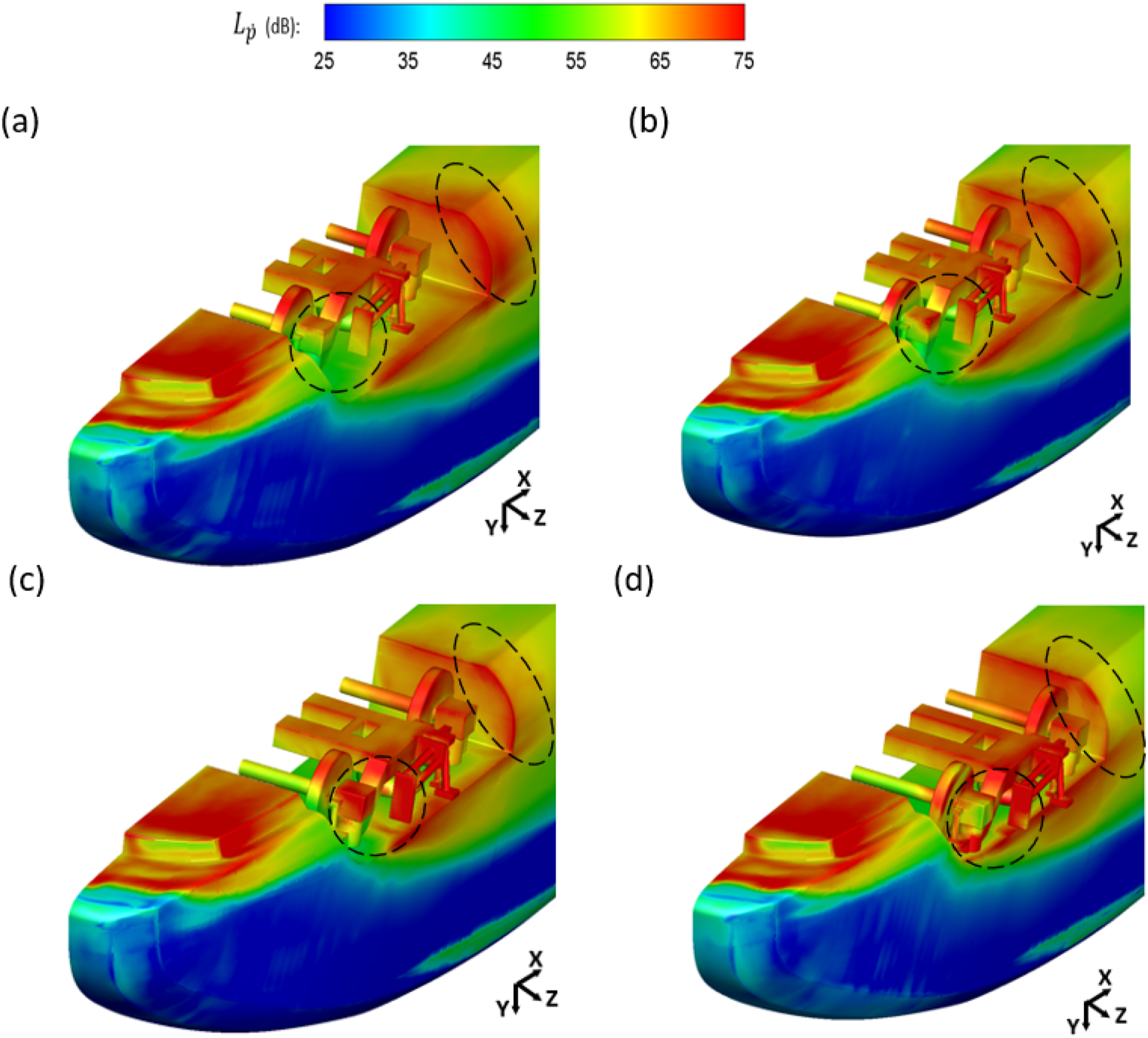$L_{\dot{p}}$ on car body and bogie surfaces for the four cases, shown in dB re 1 Pa/s; (a) Case m100; (b) Reference case; (c) Case 200; (d) Case 400.

The areas with the main differences across the four cases are highlighted by dashed-line circles. The first area is the front axle box and the endplate of the lateral damper. As the side components protrude, they move out of the cavity’s shielding and directly face the shear layer detached from upstream, as shown in Figures 4 and 5. This undoubtedly increases the $L_{\dot{p}}$ on their surface, as shown in Figure 7(c) and (d). For the area near the rear wall of the cavity, Case 400 presented in Figure 7(d) shows the highest reduction in $L_{\dot{p}}$ on the side wall of the train body. The reason is evident in Figure 4(d) to Figure 6(d), which show that the high-speed flow is deflected away from the rear corner of the cavity, thereby preventing the flow from impinging on the side surface of the car body behind the cavity. However, this results in an increase in the area with strong noise sources on the surface of the side components. Except for the areas within the black circles, the difference of noise source strength is insignificant across the four cases. The net change in noise, due to this reduction and increase, will be discussed in the next section.

Aeroacoustic results

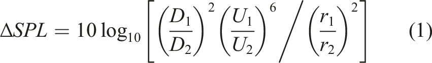
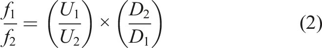
To predict the far field pressure, the fluctuating pressure recorded on each surface element is utilized as the input for the FW-H equation.^{8,10,18,20–23} After obtaining the sound pressure level (SPL) at a receiver location from the reduced-scale simulation model, the results are scaled up to the full-scale situation by applying the following equations¹⁰:

∆ S P L = 10 \log_{10} [{(\frac{D_{1}}{D_{2}})}^{2} {(\frac{U_{1}}{U_{2}})}^{6} / {(\frac{r_{1}}{r_{2}})}^{2}]

(1)

\frac{f_{1}}{f_{2}} = (\frac{U_{1}}{U_{2}}) \times (\frac{D_{2}}{D_{1}})

(2)

where

∆ S P L

is the adjustment in SPL, and

\frac{f_{1}}{f_{2}}

is the adjustment in frequency. Subscript 1 denotes the full-scale situation, while subscript 2 represents the scaled model.

D

is the geometry dimension,

U

represents the flow speed,

r

denotes the distance between the receiver and the noise source and f is the frequency. The speed exponent is taken as 6, as found in previous experimental research^5,16,24 Although quadrupole noise is a potential source when the train runs at 400 km/h, it remains insignificant according to the study by Lauterbach et al.¹⁶ Their research also indicates that the velocity exponent stays close to 6 across a wide range of Mach numbers, up to 0.3. According to the scales of the geometry and speed presented above,

∆ S P L

is 84.3 dB and the frequency ratio is 0.92. To allow for the use of the half-width model, the final values of sound pressure are combined with the results for an image receiver on the opposite side of the train.

Noise spectra

The SPL is assessed at a receiver placed 20 m from the bogie centre in the Z direction. This distance is chosen to ensure it is in the acoustic far field, given this distance exceeds the acoustic wavelength at 20 Hz, the lowest frequency of interest. For simplicity, the calculations are based on free-field Green’s functions, which neglect the acoustic effects of the train geometry; in practice these would lead to reflection and scattering of the sound.

Figure 8 displays the noise spectra obtained for the four cases. Initially, the power spectral densities (PSD) were obtained utilizing Welch’s method, employing a Hanning window with a 50% overlap for each segment. With 19 to 22 segments, each approximately 0.4 s long, the frequency resolution is 2.5 Hz. Subsequently, these narrowband noise spectra are integrated to give 1/3 octave band levels. The spectra are broadband and predominantly characterized by low frequencies below about 300 Hz.

Figure 8.

Noise spectra (full scale) at 20 m for the four cases; (a) Bogie; (b) Car body.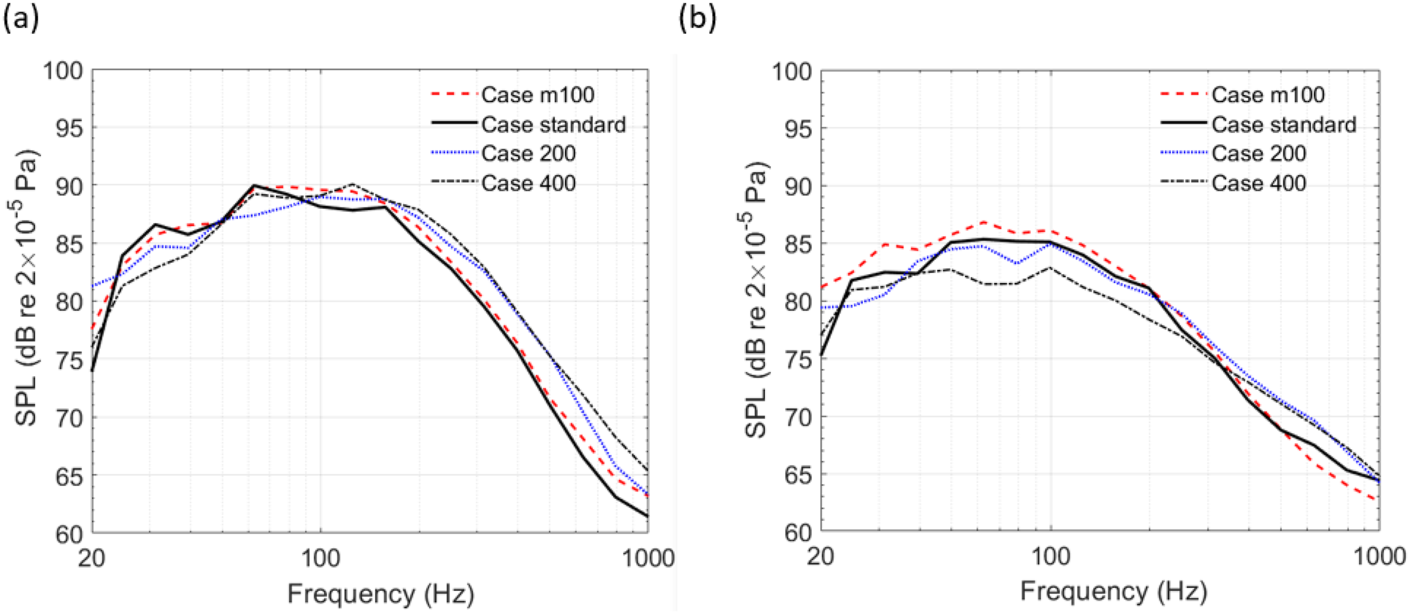

In Figure 8(a), the bogie noise spectrum of case m100 is very similar to that of the standard case. This indicates that the shortened bogie side components are unaffected, as they remain fully shielded and the velocity inside the cavity is very low, as shown in Figure 4(a) and (b). This is also confirmed by the noise source distribution on the bogie side components, as shown in Figure 7(a) and (b). However, with an increase in the protrusion of the side frame, the SPL from the bogie decreases at frequencies below approximately 160 Hz, while it increases at frequencies above this. In Figure 8(b), the cavity noise spectrum of case m100 shows slightly higher SPL at low frequencies compared to the standard case. This is due to the shortened side components exposing more of the rear cavity wall to the upstream shear layer, as shown in Figure 5(a). Similarly, as in the bogie noise spectra, as the side components protrude, the SPL increases at low frequencies and decreases at high frequencies. These differences occur when the side components extrude because, as the side components protrude further, the influence of the detached shear layer diminishes, resulting in reduced surface flapping at low frequencies. Conversely, the impingement of the free stream becomes more significant, playing a larger role at higher frequencies.

Figure 9 illustrates the overall SPLs integrated over the range 20-1000 Hz; the lower frequency corresponds to the minimum frequency of the audible range, while the upper frequency is sufficient to cover the broad spectral peak. As shown in Figure 9(a), the unweighted SPL at this receiver due to the bogie is very similar for each case. However, the SPL due to the car body decreases monotonically as the lateral extension of the side frame increases and the difference between case m100 and Case 400 is around 3 dB. Because of the monotonical change of the car body component, the total noise also follows a similar trend and the maximum difference is around 2 dB. The reason for the reduction in the SPL from the car body can be found from Figure 7, which indicates reduced pressure fluctuations at the corner of the cavity and rear part of the car body, which is a critical area for noise radiation in the horizontal direction. Although the SPLs of the car body are lower than those from the bogie, the main contribution from the car body is primarily in the vertical direction.

Figure 9.

The overall SPLs of the four cases at the side receiver at 20 m from the track centre. (a) Unweighted; (b) A-weighted.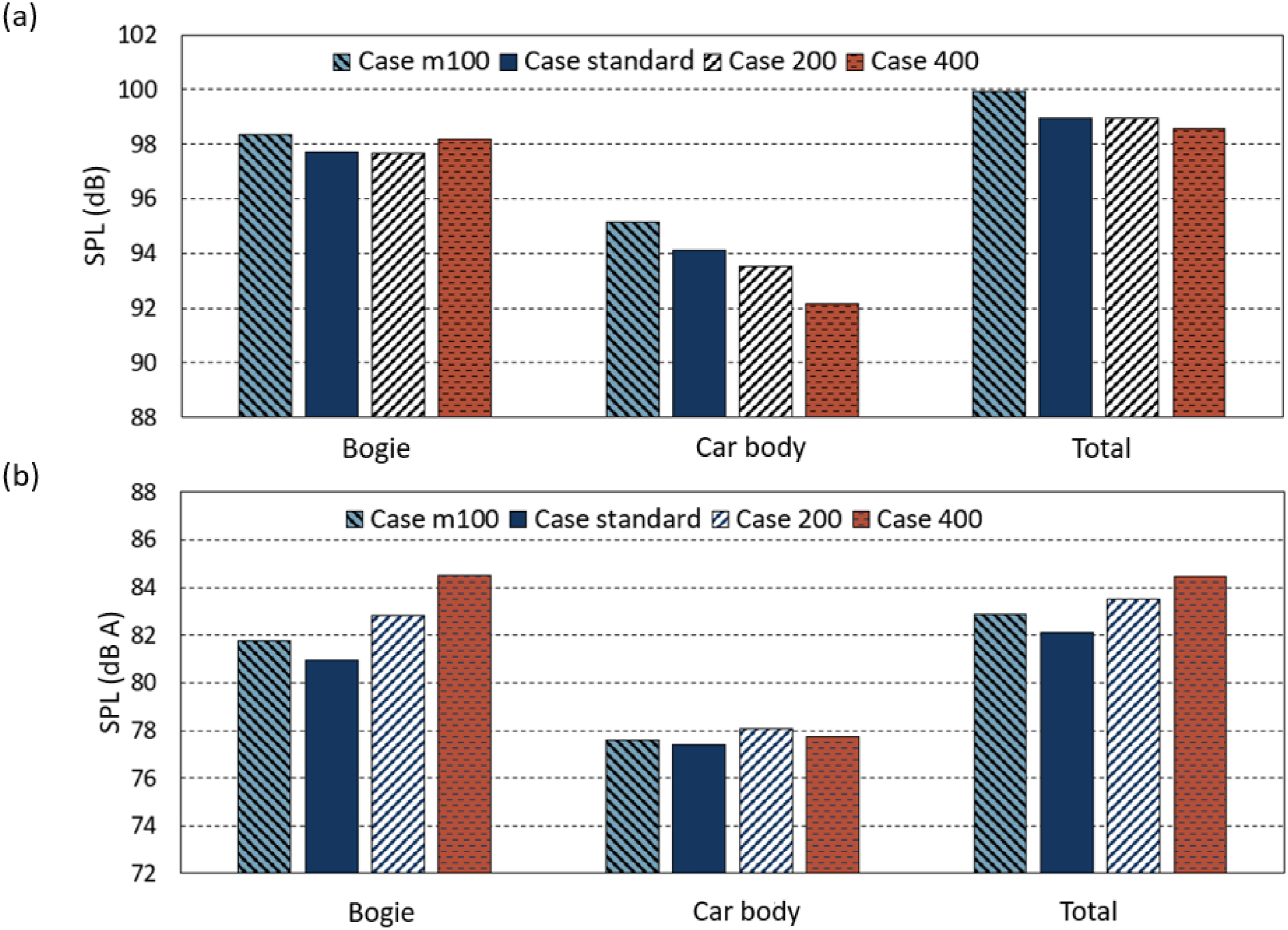

Figure 9(b) illustrates the A-weighted SPLs at the side receivers. As the A-weighting suppresses the effects of low frequencies, the contribution of high frequencies to the overall noise increases. Therefore, according to the noise spectra comparison in Figure 8, the SPL increase at low frequencies will have little effect, while the differences at high frequencies will have greater effect. The maximum difference in bogie noise is approximately 3 dB, while the total noise difference is around 2.5 dB. Therefore, the results in Figure 9(b) exhibit the opposite trend to the unweighted SPLs in Figure 9(a).

Sound power levels

To quantify the overall changes in noise caused by the position of the side components, the sound power levels (SWL) generated by various components are calculated. These results should be largely independent of the scattering effect of the car body. To determine the sound power, the total mean-square pressure $\bar{p^{2}}$ is obtained in the frequency range from 20 Hz to 1000 Hz at 486 receiver points. These are distributed on a sphere of radius 20 m, centred at the centre of the bogie. The SWL is determined in accordance with ISO 3745²⁵ but using many more receiver points for increased accuracy. It is determined independently for car body sources and three groups of bogie components: the upstream and downstream ‘dynamic systems’, comprising the wheelset and axlebox, and the ‘frame system’, including the frame, the side dampers, and the air spring, as illustrated in Figure 1.

Figure 10 shows the A-weighted SWL of these components for the four cases, expressed in dB re $10^{- 12}$ W. The difference between the SWLs of the car body for the reference case and Case 400 is approximately 2 dB. The differences between the SWL generated by the downstream dynamic system in the various cases are less than 1.5 dB and the changes are not consistently monotonic. The downstream dynamic system includes the downstream wheelset and axle box. The non-monotonic differences in this section of the side components are due to its exposure to the dispersed shear layer in case m100 and the standard case. In cases 200 and 400, where the side components protrude outside the bogie cavity, they are also influenced by the wake flow from the upstream components. However, the results for the upstream dynamic system and the frame system increase significantly as the bogie side frame is moved outwards, with differences of more than 5 dB. The frame system includes the air spring, the side dampers, and the bogie frame. When the side components protrude outward, they no longer receive shielding from the bogie cavity and directly face the shear flow, as shown in Figures 4–6. Therefore, the pressure fluctuations on the component surfaces are increased, as seen in Figure 7. The difference between the total A-weighted SWLs of the reference case and Case 400 is around 2.9 dB. A similar trend can be found between the total A-weighted SPL in Figure 9(b) and the total SWL in Figure 10.

Figure 10.

Sound power levels generated by different components of the four cases (A-weighted).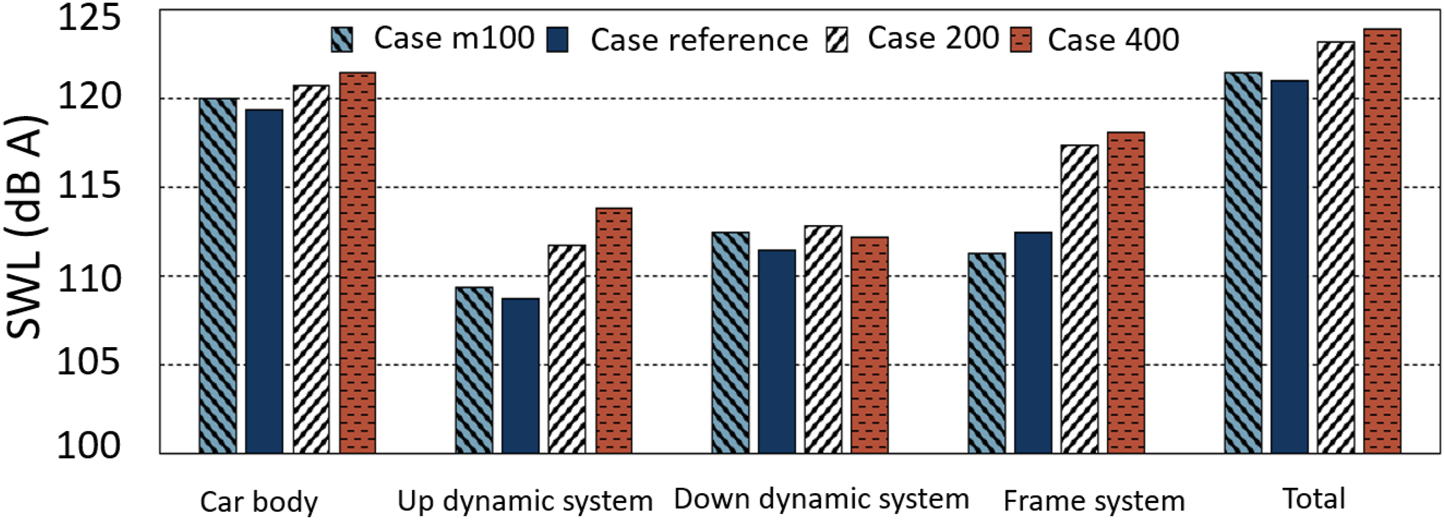

Conclusions

The impact of the lateral position of the bogie side components on the generation of aerodynamic noise in the bogie region has been investigated through numerical simulations. Four configurations were considered, with side components progressively shifted outward. Analysis of the results leads to the following conclusions:

1. Sound pressure spectra decreased at low frequencies (below 160 Hz for the bogie and 300 Hz for the car body) and increased at higher frequencies as the side components became more exposed. This is because extending the bogie frame suppressed the effect of the detached shear layer (low-frequency phenomenon) but increased the influence of the wake generated by side components, affecting higher frequency noise.

2. When the bogie side components are shifted outwards by 400 mm, the overall unweighted sound pressure reduces by 2 dB but the A-weighted level increases by 2.5 dB.

3. The overall A-weighted sound power level (SWL) showed differences of more than 5 dB for the upstream dynamic and frame systems. The most extended configuration increased total A-weighted SWL by 2.9 dB compared to the reference case.

4. The reference case or case m100, with bogie components shielded by the cavity, is preferable for a lower A-weighted SWL. This also applies to the A-weighted SPL at the trackside receiver. However, the most extended configuration has the lowest unweighted SPL as it reduces the low-frequency noise from the detached shear layer on the rear corner of the cavity.

Footnotes

Acknowledgements

All simulations were performed on Iridis5 cluster at the University of Southampton.

Declaration of conflicting interests

The author(s) declared no potential conflicts of interest with respect to the research, authorship, and/or publication of this article.

Funding

The author(s) disclosed receipt of the following financial support for the research, authorship, and/or publication of this article: The work has been supported by the Ministry of Science and Technology of China under the National Key R&D Programme grant 2016YFE0205200, ‘Joint research into key technologies for controlling noise and vibration of high-speed railways under extremely complicated conditions’.

ORCID iDs

Yuan He

David Thompson

Zhiwei Hu

References

Thompson

. Railway noise and vibration: mechanisms, modelling and means of control. Oxford: Elsevier, 2008.

Liu

Zhang

Thompson

, et al. Aerodynamic noise of high-speed train pantographs: comparisons between field measurements and an updated component-based prediction model. Appl Acoust 2021; 175: 107791.

Zhu

Thompson

. The flow and flow-induced noise behaviour of a simplified high-speed train bogie in the cavity with and without a fairing. Proc Inst Mech Eng F J Rail Rapid Transit 2018; 232(3): 759–773.

Thompson

Latorre Iglesias

Liu

, et al. Recent developments in the prediction and control of aerodynamic noise from high-speed trains. Int J Real Ther 2015; 3(3): 119–150.

Latorre Iglesias

Thompson

Smith

, et al. Anechoic wind tunnel tests on high-speed train bogie aerodynamic noise. Int J Real Ther 2017; 5(2): 87–109.

Latorre Iglesias

Thompson

Smith

. Component-based model to predict aerodynamic noise from high-speed train pantographs. J Sound Vib 2017; 394: 280–305.

Nagakura

. Localization of aerodynamic noise sources of Shinkansen trains. J Sound Vib 2006; 293(3): 547–556.

Thompson

. Numerical investigation of flow-induced noise around a high-speed train bogie in a simplified cavity. In: International Conference on Rail Transportation. Chengdu: IEEE, 2021, pp. 65–72.

Thompson

. Numerical approach for the simulation of flow-induced noise around a structure with complex geometry: high-speed train bogie in a cavity. Int J Fluid Eng 2024; 1(3).

10.

Thompson

. Aerodynamic noise from a high-speed train bogie with complex geometry under a leading car. J Wind Eng Ind Aerod 2024; 244: 105617.

11.

Minelli

Yao

Andersson

, et al. An aeroacoustic study of the flow surrounding the front of a simplified ICE3 high-speed train model. Appl Acoust 2020; 160: 107125.

12.

Q-l

Z-m

Yang

Z-g

. Noise contribution and coherence analysis of high-speed train head shape under moving slab track. Proc Inst Mech Eng Pt F: J Rail and Rapid Transit 2022: 237: 09544097221140200.

13.

Wang

Minelli

Dong

, et al. An IDDES investigation of Jacobs bogie effects on the slipstream and wake flow of a high-speed train. J Wind Eng Ind Aerod 2020; 202: 104233.

14.

Gao

, et al. Investigation of bogie positions on the aerodynamic drag and near wake structure of a high-speed train. J Wind Eng Ind Aerod 2019; 185: 41–53.

15.

Zhang

Wang

, et al. A study of the influence of bogie cut outs' angles on the aerodynamic performance of a high-speed train. J Wind Eng Ind Aerod 2018; 175: 153–168.

16.

Lauterbach

Ehrenfried

Loose

, et al. Microphone array wind tunnel measurements of Reynolds number effects in high-speed train aeroacoustics. Int J Aeroacoustics 2012; 11(3-4): 35–62.

17.

Qin

Zhou

, et al. Effect of model scale and airflow velocity on aerodynamic noise prediction for high-speed train leading car and bogie. Engineering Applications of Computational Fluid Mechanics 2024; 18(1): 2384445.

18.

. Aerodynamic noise simulation of high-speed train bogie. PhD thesis. University of Southampton, 2023.

19.

Curle

. The influence of solid boundaries upon aerodynamic sound. Proc Roy Soc Lond A 1955; 231(1187): 505–514.

20.

Wang

Thompson

. Numerical investigations on the flow over cuboids with different aspect ratios and the emitted noise. Phys Fluids 2020; 32(2): 025103.

21.

Liu

Thompson

. Numerical investigation of aerodynamic noise generated by circular cylinders in cross-flow at Reynolds numbers in the upper subcritical and critical regimes. Int J Aeroacoustics 2019; 18(4-5): 470–495.

22.

Ffowcs Williams

Hawkings

. Sound generation by turbulence and surfaces in arbitrary motion. Phil Trans Roy Soc Lond Math Phys Sci 1969; 264(1151): 321–342.

23.

Zhu

Thompson

. Flow behaviour and aeroacoustic characteristics of a simplified high-speed train bogie. Proc Inst Mech Eng F J Rail Rapid Transit 2016; 230(7): 1642–1658.

24.

Latorre Iglesias

Thompson

Muñoz Paniagua

, et al. On the feasibility of a component-based approach to predict aerodynamic noise from high-speed train bogies. Appl Acoust 2023; 211: 109536.

25.

ISO 3745:2012 . Acoustics—Determination of sound power levels and sound energy levels of noise sources using sound pressure—Precision Methods for anechoic rooms and hemi-anechoic rooms 2012.

The effect of bogie side components on the aerodynamic noise generation of the leading car of a high-speed train

Abstract

Keywords

Introduction

Computational setup

Computational model

Grid strategy and numerical set-up

Aerodynamic results

Flow field

Noise source strength

Aeroacoustic results

Noise spectra

Sound power levels

Conclusions

Footnotes

Acknowledgements

Declaration of conflicting interests

Funding

ORCID iDs

References