Sage Journals: Discover world-class research

Abstract

To meet the increasing demands for availability at reasonable cost, operators and maintainers of railway point machines are constantly looking for innovative techniques for switch condition monitoring and prediction. This includes automated fault root cause diagnosis based on measurement data (such as motor current curves) and other information. However, large, comprehensive sets of labeled data suitable for standard machine learning are not yet available. Existing data-driven approaches focus only on the differentiation of a few major fault categories at the level of the measurement data (i.e., the “fault symptoms”). There is great potential in hybrid models that use expert knowledge in combination with multiple sources of information to automatically identify failure causes at a much more detailed level. This paper discusses a Bayesian network diagnostic model for determining the root causes of faults in point machines, based on expert knowledge and few labeled data examples from the Netherlands. Human-interpretable current curve features and other information sources (e.g., past maintenance actions) are used as evidence. The result of the model is a ranking of the most likely failure causes with associated probabilities in terms of fuzzy multi-label classification, which is directly aimed at providing decision support to maintenance engineers. The validity and limitations of the model are demonstrated by a scenario-based evaluation and a brief analysis using information theoretic measures. We present the information sources used, the detailed development process and the analysis methodology. This article is intended to be a guide to developing similar models for various complex technical assets.

Keywords

Railway switch fault diagnosis Bayesian networks expert knowledge prognostics and health management

Introduction

Switches and their point machines are crucial assets of the railway infrastructure, both in terms of network availability and safety. A significant amount of delay time in railway networks can be attributed to infrastructure failures, especially railway switches.^1,2 Traditional maintenance strategies relying on preventive maintenance with fixed inspection intervals do not match the necessity for a high availability of the infrastructure at reasonable costs. To address these challenges, prognostics and health management is adopting condition-based or even predictive maintenance policies,^3,4 including diagnostic systems for automated identification of root causes of occurring faults.

Measuring motor current curves is a common approach for condition monitoring of point machines, especially in the area of anomaly detection. For example, Côme et al.⁵ first fit a hidden process regression model to a small number of current curves corresponding to a healthy switch state, then secondly use the Fisher score test to detect anomalies and applying a stochastic gradient algorithm to recursively update the model parameters. Narezo Guzman and Neumann⁶ developed and validated a data-driven anomaly detection model for current curves that accounts for temperature influences. A recent overview of existing approaches towards railway switch (incl. point machine) fault diagnosis is given in Hamdache.⁷ Huang et al.⁸ differentiate between five fault types for single-action ZD6 point machines, using dynamic time warping and reference current curves. Narges et al.⁹ focus on four common fault types for Siemens S700K point machines with the application of feature extraction and supervised learning methods. Concerning unsupervised learning, Guo et al.¹⁰ combine machine learning and engineering expertise to diagnose eight fault types of Siemens S700K point machines, using both simulated and field test data.

The data-driven approaches for point machines above are highly dependent on (partially labeled) data in terms of availability and quality, and focus on few major fault categories that are distinguishable based on (almost exclusively) current curve data. According to Silmon and Roberts,¹¹ diagnostic models should be able to deal with the full variety of faults (including rare or incipient events), be intuitive to maintenance operators and allow for automated integration into the operational workflow. Expert-knowledge based systems provide an alternative to standard machine learning approaches, that combines measurement data and other information sources without classical physical modeling of the target asset. Bayesian networks are a representative of this class of models which have been successfully applied in various fields,¹² including dependability, risk analysis and maintenance¹³ and fault diagnosis.¹⁴ They provide a probabilistic graphical modeling approach (cf. Appendix and Charniak¹⁵ for a short introduction and Koller and Friedman¹⁶ for a deeper dive), which allows for interpretable representations of complex systems.

Neumann and Narezo¹⁷ carried out preliminary work on the application of Bayesian networks for point machine fault diagnosis, outlining the conceptual approach and discussing model architecture. Almost all nodes in the graphical representation of a Bayesian network model refer to specific elements (real or abstract) or measurement data features of the switch, with specific fault states or values that occur with certain probabilities. The output is a fuzzy multi-label classification. In this context, Bayesian networks are demonstrably more powerful than standard approaches like fault trees or FMECA (Failure Modes, Effects, and Criticality Analysis).¹⁸ The different forms of causal, anti-causal (i.e., diagnostic) and inter-causal reasoning are a major strength with regard to the purpose of railway switch diagnostics.

This paper discusses the development of Bayesian network diagnostic models for point machines and mechanical track components relevant to the operability of the switch drive. The presented model is tailored specifically to NSE (Nederlandse Spoorwegen Elektrisch) point machines, but the approach can easily applied to other types of point machines as well. The goal of the model is to determine fault root causes, using human-interpretable current curve features and other influencing factors (past maintenance actions, historic switch behavior, environmental factors, railway metadata, power supply) as evidences. The output of the model, a ranking of the most likely faults with associated probabilities (fuzzy multi-label classification), is directly aimed at maintenance engineers. In contrast to previous conceptual work, the model includes all (in our view) relevant asset component and fault states, handles multiple sources of information and, most importantly, has passed a comprehensive scenario-based performance evaluation by maintenance experts.

Automated calculation of the required human-interpretable current curve features, evidence calculation and maintenance decisions based on the model output are not within the scope of this paper. First steps towards human-interpretable current curve features (e.g., humps) and the integration of the presented diagnostic model into an operational environment are described in Narezo Guzman et al.¹⁹

The remainder of this paper is structured as follows. The next section gives an overview of the data and other sources that serve as a basis for the model development process. The third section describes the development process itself, while section four presents the resulting diagnostic model and the output of the last iteration of the evaluation. In section five, a deeper analysis of the model’s behavior in terms of information theoretic measures is carried out. The last section contains conclusions on the presented work and gives an outlook onto options for further development.

Information sources

Historical data

The vast majority of historical current curve data is generally unlabeled. For this research work, there were a number of selected reports of maintenance actions available, comprising information about 17 switches over the course of 2012 until 2021. Figure 1 displays the number of reports addressing point machine health, grouped into aggregated fault categories. The high number of reports in the category “Adjustment” are partially due to the fact that a number of different maintenance actions can fall under that label. In addition, the label was sometimes found to be used by mechanics as a default if the performed maintenance actions are difficult to categorize or would require a lengthy documentation otherwise.

Figure 1.

Number of considered reports per fault category.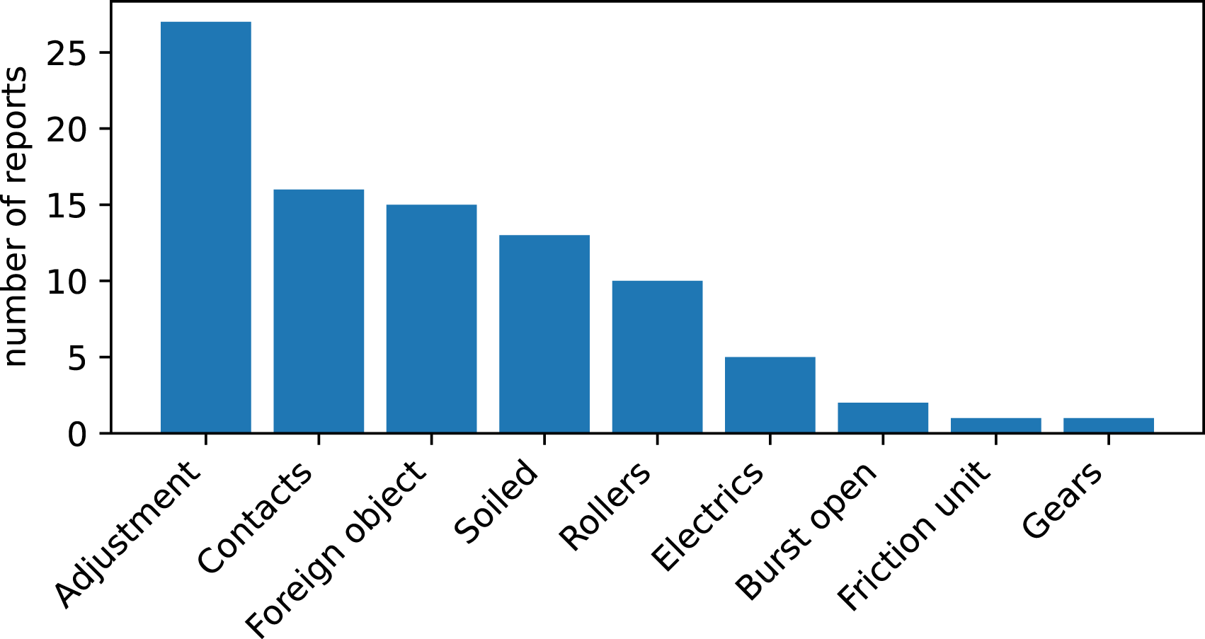

Experimental data

To challenge the lack of a precisely labeled database, series of experiments were conducted at Strukton Rail’s switch maintenance training facility in Amersfoort. Ten different fault types in various forms were subsequently purposefully introduced onto a test switch while measuring the motor current curves for both directions of the switch blade movement, as well as a reference curve just before the introduction of each fault (and after removal of the previous fault).

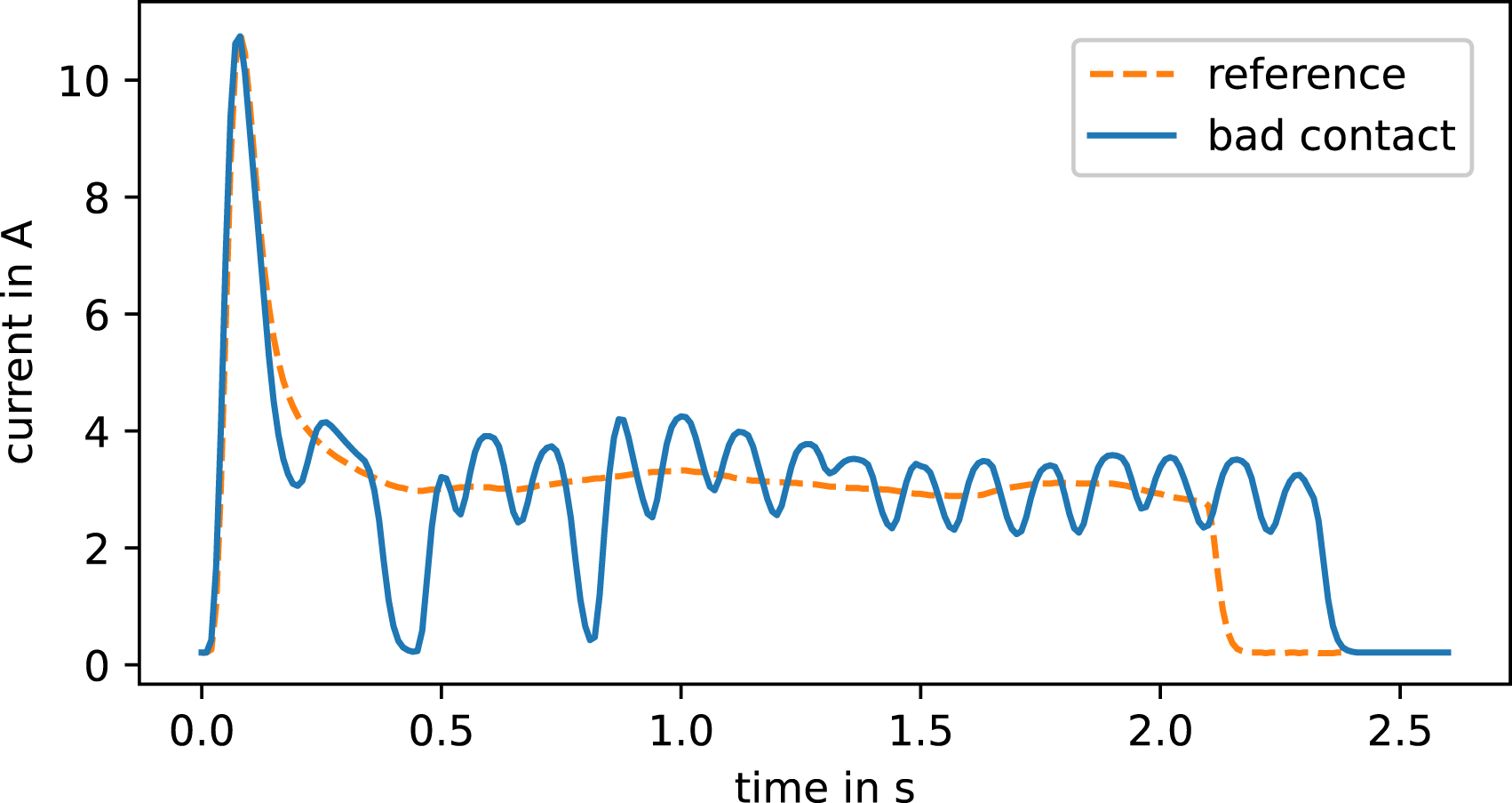
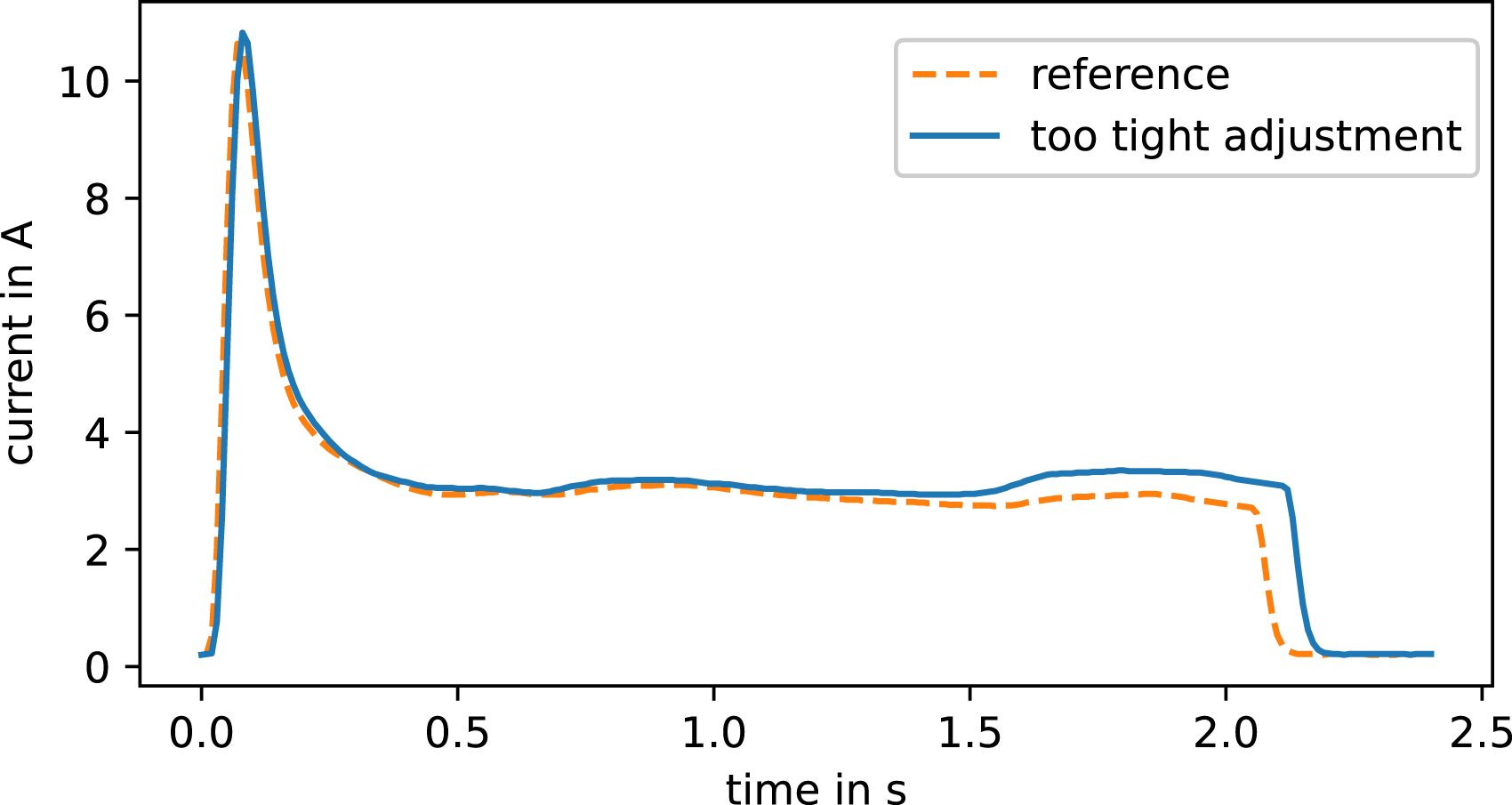
Figure 2, for example, shows the experimental simulation of a bad contact in the power supply, resulting in the current curve depicted in Figure 3. In Figure 4, the movement rods are maladjusted such that the closing switch blade closes too tight toward the stock rail, resulting in a heavy closing and thus increased current level during the locking phase of the current curve. At approximately 2.2 s, the second set of contact fingers switches over and the point machines shuts down. In this moment, the increased current level causes electrical sparking. This phenomenon burns the surface of the contact fingers in the long term and thus shortens their lifetime. In general, there are several examples of such long-term fault propagation in railway switches.

Figure 2.

Experimental simulation of a bad contact in the power supply.

Figure 3.

Current curve of the experimentally simulated bad contact in Figure 2. The disruption of the power supply causes the current to drop and momentarily slows the movement of the motor.

Figure 4.

Current curve with a too tight adjustment of the movement rods. This causes a heavy locking of switch blades, which is visible in the data as a hump between 1.5 s and 2.2 s.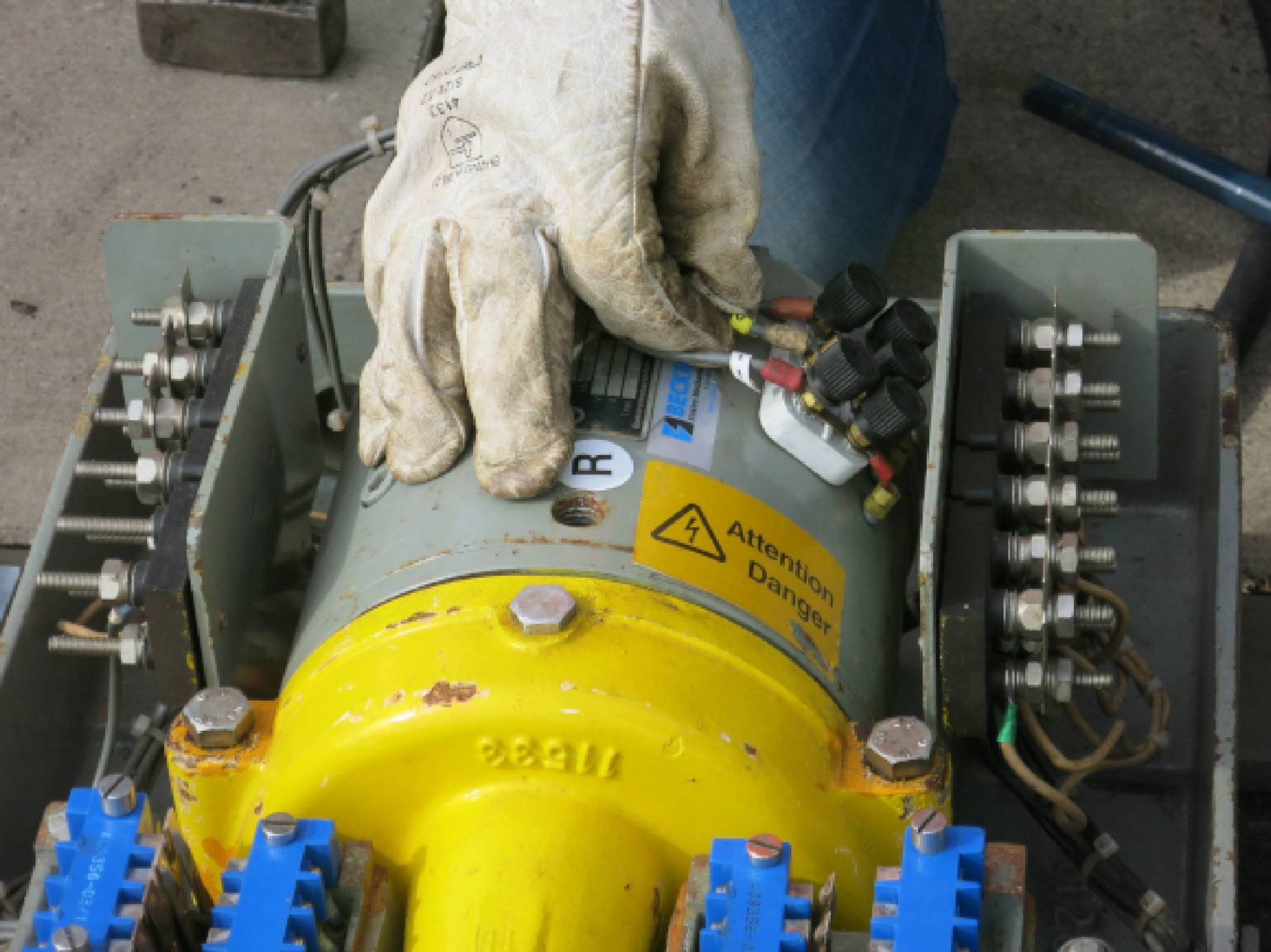

Expert knowledge and other sources

Reference values for fault occurrences in railway switches can be found in Bemment et al.,²⁰ Rama and Andrews,²¹ Hassankiadeh²² or Kassa,²³ for instance. However, these numbers are not necessarily transferable to NSE point machines and there is often a high level of aggregation, or only the most common fault types are considered.

The manufacturer Voestalpine WBN provides recommended maintenance actions and intervals in their manual²⁴ for NSE point machines. These give an indication on the expected occurrence and criticality of certain faults, as well as the level of detailedness a diagnostic model would need to provide.

A common approach to systematically catalog different components of a complex system and their possible faults is to conduct a FMECA. Kassa²³ gives an comprehensive introduction to the method and applies this technique on switches (incl. track superstructure and drive) to determine critical faults and support maintenance planning on a high level. For the development of the model presented in this paper, Strukton Rail provided a detailed FMECA conducted specifically for NSE point machines.

Even if the above sources all provide important insights towards components, fault states and their likelihoods, there is no information on the detailed interaction of influencing factors, measurement data (features) and fault occurrences, giving rise to the need for additional inputs for the modeling process. In this regard, although not tangible, the most valuable and important information source for building a detailed diagnostic model as presented below finally turned out to be expert knowledge from data and maintenance analysts at Strukton Rail. These have many years of working experience in the operational maintenance of switch drives and their expertise includes, among other things, switch measurement data analysis, assignment and execution of maintenance actions and training of field mechanics.

Development process

Cai et al.¹⁴ reviews a number of Bayesian network applications for fault diagnosis and presents a general workflow for developing such models, data-driven or manually. Due to the information sources available for modeling purposes as presented in the previous section and in regard of the lack of a larger amount of labeled data, a data-driven approach is not feasible here. Lack of labeled data is a common problem in prognostics and health management in the railway infrastructure sector, requiring methods that can work with limited data. The following section discusses the stages of manual model development for complex technical assets and outlines the design decisions specifically made for the diagnostic model in this paper.

The development process (violet) summarized in Figure 5 is based on the available information sources (yellow) discussed in the previous section. The first step is to determine the structural design and temporal scope, followed by parameterization and scenario-based evaluation. These steps are iterated in close interaction with the experts until an appropriate model structure for the application is found and the evaluation shows the desired accuracy of results. The output of the development process is the model itself and the results of the last iteration of the evaluation (blue). Subsequent to development, an entropy analysis (green) can be conducted to gain further insights into the model’s working.

Figure 5.

Development process with information sources, resulting model and subsequent analysis.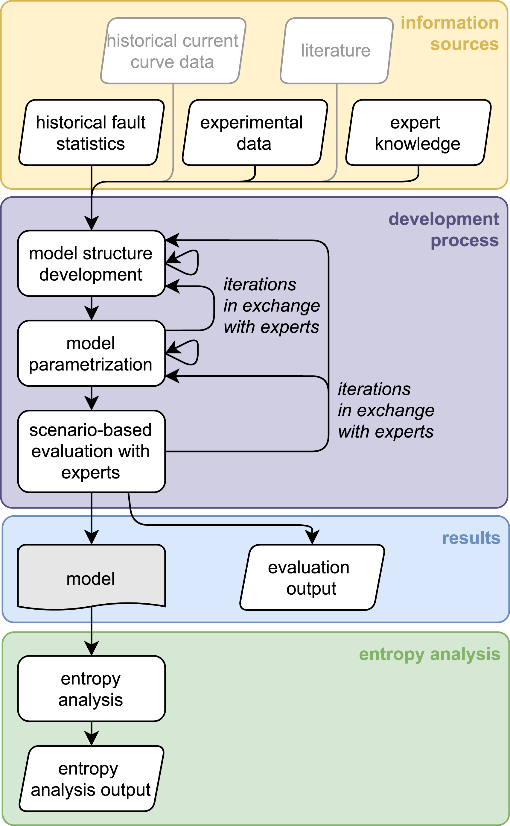

Structural design

Bayesian networks are probabilistic graphical models whose structure is that of a directed acyclic graph. In diagnostics, the asset and its associated variables are represented by nodes (e.g., components or functional aspects of the switch) with states or values (e.g., healthy and fault states) that occur with certain probabilities. Cause-effect relations are modeled by the directed links between nodes (for more details, see Appendix). The nodes can be categorized into three layers, influencing factors (e.g., environmental conditions) which are typically root nodes, then the target nodes which represent the switch with its fault types and finally a layer of observable symptoms (e.g., measurement data features). Each layer can have a depth of more than one, e.g., primary target nodes are summarized into aggregated nodes with their own fault types. This strategy can be used to model larger overall components, functionalities or behaviors of the switch. It also simplifies parameterization by reducing the total number of parameters and the complexity of parameterization for each individual node (by reducing the number of parent nodes).

In a component-based view of assets, the asset is modeled as a collection of all its physical components as nodes and faults as states similar to FMECA. This provides a detailed, complete representation of the asset regardless of data availability, but faults can be difficult to assign to individual components and the linkage to symptoms is not straightforward. Further, because of its completeness, the representation of the asset may include faults that have no symptoms at all in the available data. From a functional view, the asset is modeled by its (sub-)functionalities as nodes and its behavior as states. This is closer to data-driven approaches such as neural networks, where the diagnosis focuses on very few broad fault categories that describe typical behavior patterns. The representation of the asset is then less detailed and prone to incompleteness, but also closer to the symptoms in the measurement data. Influencing factors, on the other hand, can be more difficult to handle if they affect specific components only. In practice, a good trade-off between a component-based view and a functional view has to be found, which often goes hand in hand with the choice of granularity of the model. On the one hand, the information provided about target nodes must be sufficient for maintenance engineers to distinguish between phenomena that have different influencing factors or symptoms. On the other hand, too much detail unnecessarily complicates the modeling process, increases the size of the model, and does not add to the diagnostic power as long as the evidence that can be obtained in practice does not contain information that differentiates at the same level.

For the model presented in this paper, the primary target nodes are components of larger granularity (e.g., clutch as a whole instead of all its individual components) and the fault types can have a more functional interpretation (e.g., clutch slipping too late). Some functionalities or switch behavior are captured through aggregated target nodes to help bridging the gap towards the symptom nodes. The granularity follows the approach “As fine as necessary, as broad as possible”.

Further, this stage of the development process also includes a verification of the structural completeness of the model by the experts, potentially in parallel with a preliminary parameterization for demonstration purposes.

Temporal scope

Comprehensive modeling of a technical asset can require consideration of the evolution of measurement data, asset behavior and influencing factors over time. Dynamic Bayesian networks essentially duplicate a static network for a fixed number of time slices (e.g., over a fixed number of equidistant past measurements) and define connections between them. While this is a very elegant way of modeling short-term dependencies, it is not a feasible approach for larger networks over a larger number of time steps.

The diagnostic model in this paper is applied to single current curve measurements, which typically occur at irregular intervals in the double digits per day. Temporal effects can span from a few days (features) to a few months (fault propagation), making the use of dynamic Bayesian networks inappropriate. Instead, current curve features are computed and tracked (outside the model) over a longer period of time, i.e. over several current curves. Past faults can then be incorporated via specific nodes in the network representing the historical switch behavior in an aggregated way, as it is relevant for diagnostic reasoning in the present situation.

Parameterization

In a Bayesian network, prior probabilities must be specified for all nodes and conditional probability tables for all other nodes (see Appendix). An inference algorithm then calculates the probability distributions for all nodes and updates them as evidence is obtained. An approach to significantly reduce the parameterization effort by reducing the number of free parameters is to use NOISY¹⁶ nodes, where essentially each parent node’s influence on the given child node is considered independently. In the case of knowledge engineering applications, Zagorecki and Druzdzel²⁵ argued that in about 50% of all node distributions, NOISY distributions can replace full conditional probability tables very well. Furthermore, in manual parameterization, the individual effects of parent nodes on child nodes may be well known (to application experts or via data), but their joint influence can be much harder to estimate. Therefore, the advantages of this simplification often outweigh the disadvantages, especially when applied in consideration of the underlying causalities.

Therefore, for the presented model, NOISY distributions are preferred, unless there are direct logical interactions between the parent nodes that require explicit modeling. Further, relevance tree inference²⁶ is used to update the probability distributions in the model, which is a commonly implemented exact probabilistic inference algorithm.

Scenario-based evaluation

After iterations between model structure development and parameterization, the performance of the model needs to be systematically evaluated to provide a reasonable level of confidence before implementation into running operations.

From a data-driven point of view, the standard approach to model validation is to test the model on a large, labeled (i.e., all states of all nodes are known) data set that was previously unknown to the model, and to statistically analyze the model’s performance. However, manual model development and the use of expert knowledge is motivated by the lack of such data sets in the first place. An alternative is scenario-based model evaluation, where experts access the model output for a limited number of real or hypothetical use cases. A scenario is considered accepted, if the model output matches the possible fault cause(s) for the given evidence set and their approximate probability (or ranking) based on the expert’s judgment (in terms of fuzzy multi-label classification). For real-world examples, the model may indicate a larger number of possible faults than the actual outcome, as the given evidence may not be sufficient to rule out all non-relevant causes. In this case, the developer can investigate adding more evidence nodes to the model structure (e.g., additional sensor data if available) to improve the diagnostic power of the model. Scenario-based evaluation is not comprehensive (not covering all possible combinations of evidences due to exponential growth of numbers) and only qualitative (no probability threshold for fault identification and confusion matrix), but can demonstrate the model’s credibility in the absence of sufficiently (labeled) validation data.

In the case of our model, the validation included 39 main scenarios (mostly based on real-world examples), with sub-scenarios to test slight variations of the evidence sets, e.g., to analyse different influencing factors or information availability. In total, 55 different evidence sets and their respective model outputs were evaluated.

Cai et al.¹⁴ also mention a number of other more general approaches to Bayesian network verification and validation that are not use case specific. These are discussed in the analysis section of this paper.

Model and exemplary scenarios

The outputs of the development process in Figure 5 are the (finalised) diagnostic model and its performance on the evaluation scenarios in the last development iteration (both presented below). The experts’ expectations on performance for an iteratively, manually developed model are fully met, such that the next step towards an operational system, the test-wise implementation in a real-world environment, can be approached in the future.

Model

Figure 6 shows an overview of the node groups of the diagnostic model and their connections. The full model comprises 66 nodes, 178 states, 105 links and 661 free parameters. Describing the model layer by layer, the node groups of influencing factors (right hand side in Figure 6) are the following:

• Railway metadata (RM): Information such as load, age of different components, or reports on drive-up incidents.

• Environmental factors (EF): Weather and climate information.

• Maintenance (M): Time since last maintenance of the point machine, track components or tamping.

• Historic switch behavior (HSB): Past behavior of the switch, as calculated by the diagnostic model itself in the past over a longer period of time, affecting the probability of current primary faults because of accelerated degradation effects. For instance, this could be a long-term too high closing current resulting in faster abrasion of electrical contacts or impaired blade lifting resulting in increased stress on the slide chairs.

• Power supply (PS): As the power supply is not measured in our application right now, meta data on the power supply such as competing switches that cause dips in the supply is used. The power supply nodes, essentially functioning as target nodes in that moment, are partially also directly influencing the symptom nodes and thus can explain away suspicious evidence in the symptom nodes. However, strictly speaking, variations in the power supply are not considered as faults from a maintenance operator’s point of view.

Figure 6.

Overview of the node groups of the diagnostic model and their connections. The arrow directions are determined by the causal relations between the node groups, just like the parent-child node connections in the full model.

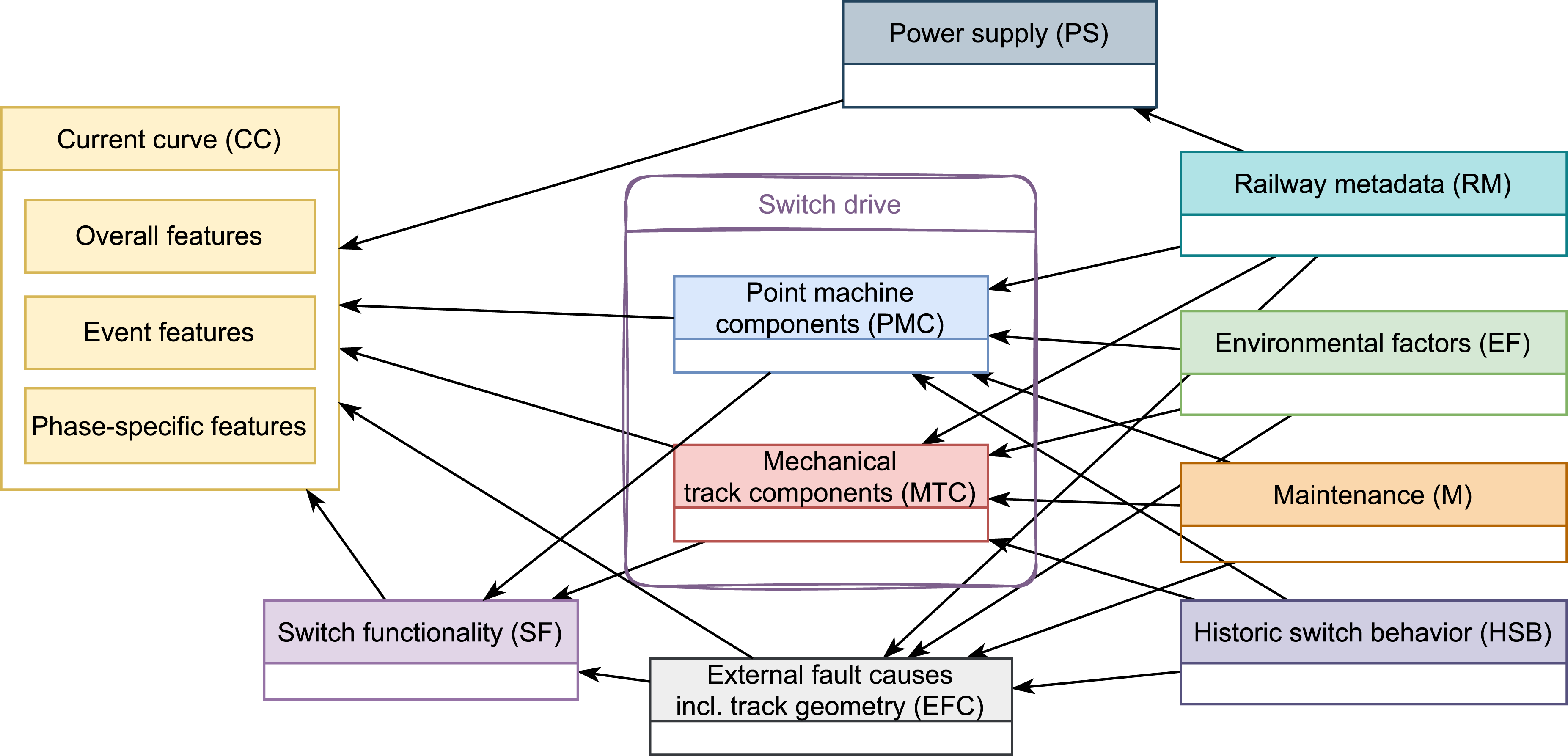
The target nodes (middle of Figure 6) are divided into the groups below. The first three groups contain the primary target nodes that are of most interest to maintenance operators, in total 20 nodes with 38 fault states (excluding the states related to healthy condition of nodes).

• Point machine components (PMC): Components that belong to the NSE point machine itself.

• Mechanical track components (MTC): Components of the track superstructure (rods, switch blade rollers, …) that are involved into the switching process.

• External fault causes (EFC): For example pollution. Track geometry is sorted into this category as well, as in practice, maintenance for point machines and track health are typically separate operations.

• Switch functionality (SF): Aggregation of nodes from the above mentioned groups, describing resulting (sub-)functionalities of the switch in terms of its proper working.

All symptom nodes belong to the current curve (CC) group (left hand side in Figure 6), where each node describes a current curve feature with its specification as (discrete) states. NSE current curves are typically segmented into inrush, unlocking, movement and locking phase. Consequently, the features used in the diagnostic model are divided into the following subgroups:

• Overall features: Features that describe the current curve as a whole, or spread out over the whole length of the curve like small oscillations, for example.

• Event features: Sudden events such as an early breakdown of the current curve, where it can be relevant to know in which phase these events occur.

• Phase-specific features: Features that are calculated for specific phases only, like different types of humps, for instance.

All features describe characteristics of the current curve that are visible and interpretable to the human eye. The model thus does not overlap with research work in the area of feature engineering, clustering and other methods to extract interpretable measurement data characteristics, but uses their results (and other sources) for diagnosis of root causes directly addressed to maintenance operators.

Exemplary scenarios

To illustrate the behavior of the model and its reasoning approach, including a discussion of its capabilities and limitations, two prime examples from the last round of iteration during the scenario-based evaluation are presented below. For reasons of space, only the fault states relevant to the scenarios are shown here. In application, the most likely failures would be presented to the maintenance operator in descending order of probability as a decision support tool.

The first exemplary evaluation scenario includes the following evidence sets, with a reference current curve and the relevant resulting faults and their probabilities summarized in Figure 7.

• Base scenario: Information only on the features of the given current curve, including an overall hump in the movement phase, while all other features are within the normal range.

• Variant (a): Base scenario plus information on recent maintenance on the mechanical parts of the track.

• Variant (b): Base scenario plus no recent tamping, high load, and both bad substructure and bad ballast quality.

Figure 7.

Reference current curve and evaluation results for different evidence sets in the first scenario.

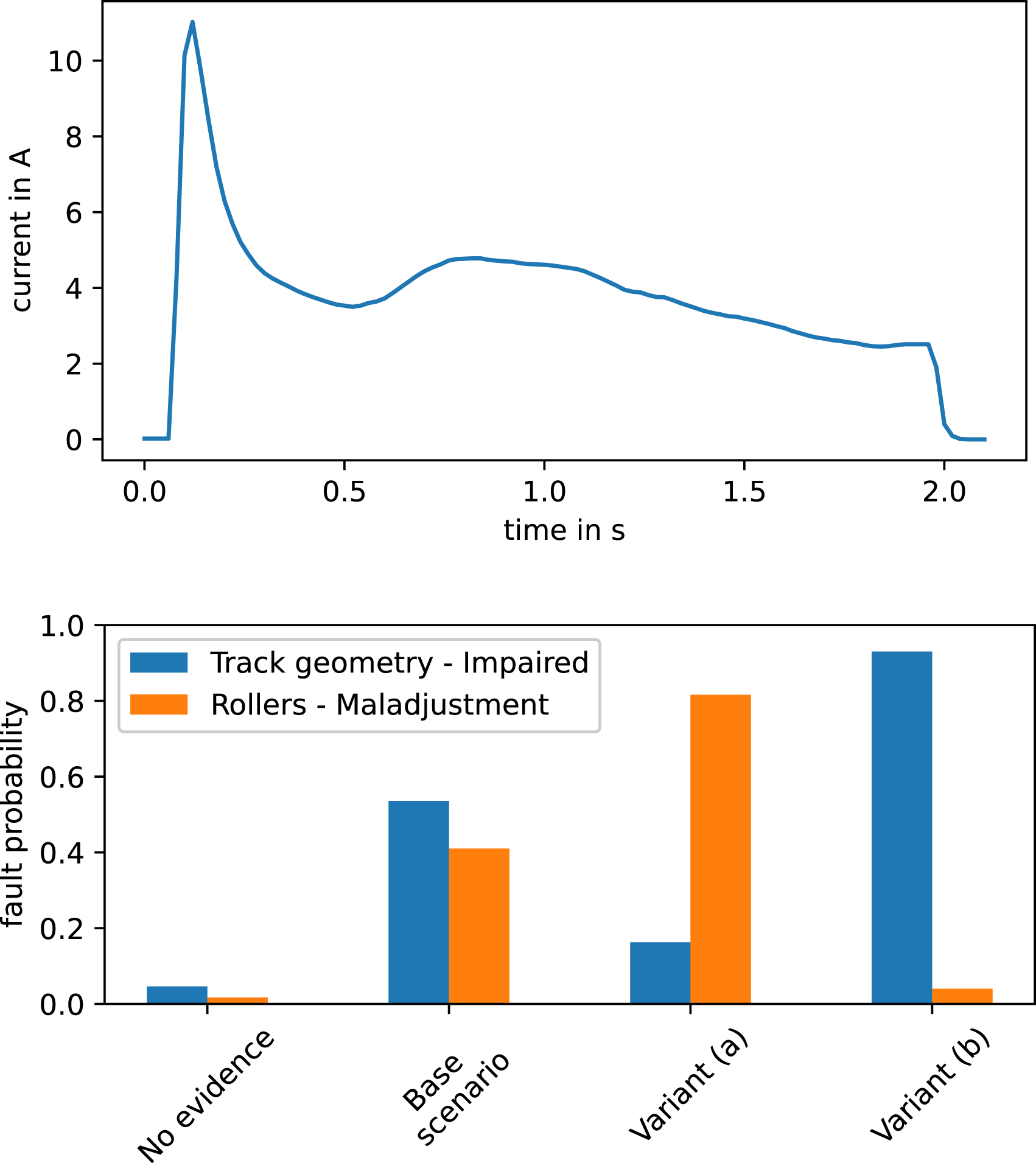
Without any evidence, all fault states of the target nodes naturally have relatively low probabilities. Given the current curve evidence in the base scenario, the model diagnoses either an issue in track geometry or a maladjustment of the rollers, while other faults do not significantly gain in probability. This is quite plausible, as the hump in the current curve is most likely caused by an increased mechanical resistance during the movement phase without further differentiating between the actual reasons for this resistance. Assuming recent maintenance on the mechanical parts of the track (variant (a)), the rollers are the more likely fault. This is due to the fact that, in practice, maintenance on track components often means that the rollers need to be readjusted, but challenging environmental conditions during the maintenance time window often negatively affects the quality of maintenance, potentially resulting in an imperfect roller adjustment. On the other hand, all influencing factors in variant (b) together would strongly indicate an impaired track geometry, thus explaining away a potential roller maladjustment.

The second scenario includes the following evidence sets, with a reference current curve and the relevant resulting faults and their probabilities summarized in Figure 8.

• Base scenario: Information only on the features of the current curve, with a humped inrush and locking phase. Otherwise, all current curve features are inconspicuous.

• Variant (a): Base scenario plus additional information on build-up precipitation inside the point machine.

• Variant (b): Variant (a) plus historical heavy locking of the switch.

Figure 8.

Reference current curve and evaluation results for different evidence sets in the second scenario.

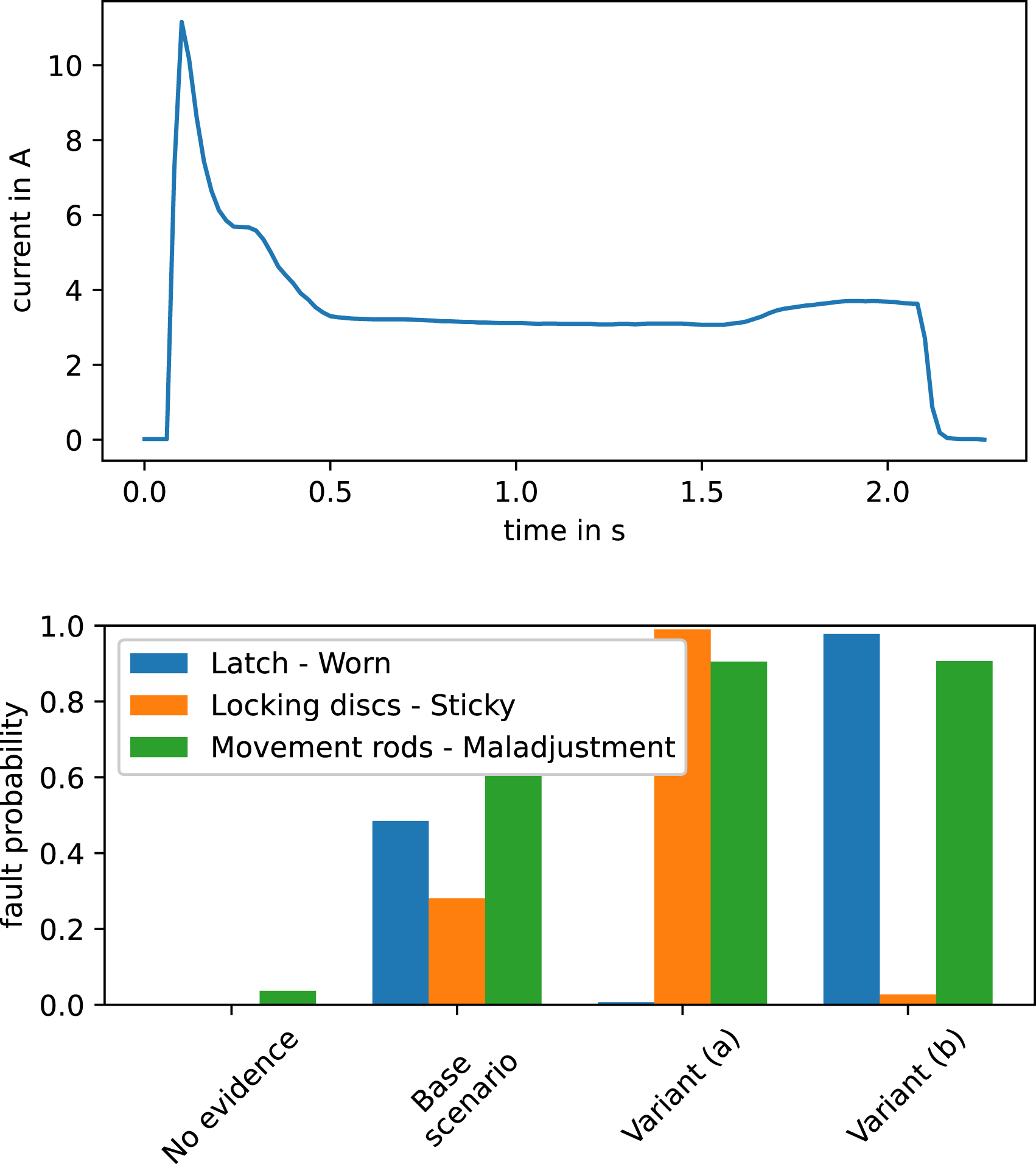
In the base scenario, the model interprets the humped locking as a maladjustment of the movement rods, while the hump in the inrush could be caused by a worn latch or by sticky locking discs. If there are information on precipitation build-up inside the point machine (variant (a)), the locking discs are diagnosed as the more likely root cause, as penetrating water can cause these to stick together. In case of a long-term problem with heavy locking of the switch in the past (variant (b), e.g., the movement rod maladjustment persisted over some time), the evidence for a worn latch overrules the previous information.

Both a worn latch and sticky locking discs show the same symptom (humped inrush) in the current curve measurement data, such that each of them can explain away the other and the model tries to decide between both root causes. In case of indecision, the probabilities of both faults are around 50%. Meanwhile, the maladjustment of the movement rods is connected to a different symptom (humped locking), such that this fault is accurately diagnosed at the same time. The model does not weigh the maladjustment against the other faults and the probability of maladjustment is not affected by additional evidences purely related to the other faults.

Multiple simultaneously occurring (more or less severe) faults are a not uncommon in point machines and in the case of different symptoms, these can be diagnosed at the same time. In the case of multiple possible root causes for the same symptom, explaining away is a great strength of Bayesian networks, helping to rule out less likely root causes. At the same time, however, it can be a disadvantage if two or more faults with the same symptoms actually occur simultaneously. In this case, it is very helpful to add further evidences to the model, as in the variants above. Generally speaking, the more information sources are available as evidences, the more reliable and less sensitive to inaccurate parameterization the model’s results are, as it is less likely that different faults have exactly the same set of influencing factors and symptoms.

Entropy analysis

Not at least because of the sheer amount of (even realistically) possible evidence sets, scenario-based evaluation as discussed in the previous section is a highly selective process. The approach directly shows how the model works, is easily understood by maintenance operators (i.e., experts), and is undoubtedly an important part of the manual development process. Nevertheless, there can be no claim to completeness.

Another way to investigate the behavior of a Bayesian network model is to apply more general tools and measures from the area of information theory, such as link strength, log-likelihood or entropy. To complement the previously discussed scenarios with their various evidence sets, this section takes a closer look at the pairwise connections between evidence nodes and target nodes (regardless of whether they are directly connected by a link in the network or not).

The entropy²⁷ H(X) for a given random variable X with probability distribution p is a measure for uncertainty with

H (X) = - \sum_{x} p (x) \log (p (x)) \geq 0 .

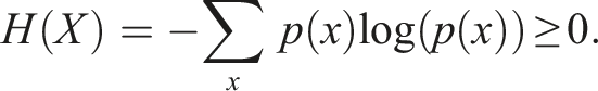
The conditional entropy of X given another random variable Y is

H (X ∣ Y) = - \sum_{x, y} p (x, y) \log (p (x ∣ y)) \leq H (X) .

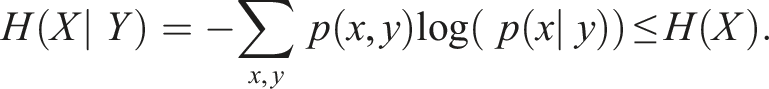
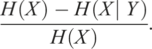
Hence, the addition of information Y never increases the uncertainty in X. Considering the proposed diagnostic model, we are interested in the relative reduction of the entropy of X (e.g., a switch component with its fault states) through Y (e.g., a measurement feature), which can be calculated as

\frac{H (X) - H (X ∣ Y)}{H (X)} .

Table 1 exemplary shows the relative entropy reduction per evidence node for the target nodes of the evaluation scenarios presented in the previous section, if this value is greater than 0.01% (otherwise omitted for reasons of space). Note that the values refer to nodes with all their states together, while the scenarios only investigated specific fault states.

Table 1.

Target nodes from the two exemplary scenarios and their relative entropy reduction per evidence node in descending order, if greater than 0.01% (otherwise omitted for reasons of space). The nodes in the table are preceded by their node group abbreviation according to Figure 6.

Target node	Evidence node	Relative entropy reduction
EFC - Track geometry	M - Tamping	10.95%
	CC - Movement shape	10.93%
	CC - Locking shape	1.12%
	RM - Load	0.37%
	RM - Substructure quality	0.11%
	RM - Ballast quality	0.11%
	EF - Ground temperature	0.05%
MTC - Rollers	CC - Movement shape	63.87%
	M - Maintenance (track-side)	4.58%
	M - Tamping	3.88%
	CC - Locking shape	0.07%
MTC - Movement rods	CC - Locking shape	88.58%
	M - Tamping	7.15%
	M - Maintenance (track-side)	0.46%
	RM - Switch burst open	0.06%
	CC - Movement shape	0.03%
	RM - Load	0.01%
	CC - Flat spot & increased duration (worsening)	0.01%
PMC - Latch	CC - Inrush shape	76.52%
	HSB - Blade locking (historical)	24.73%
	RM - Age (PM)	3.20%
	CC - Stable high current	0.37%
PMC - Locking discs	CC - Inrush shape	80.86%
	PM - Age (PM)	5.47%
	EF - Precipitation build-up inside PM	0.02%

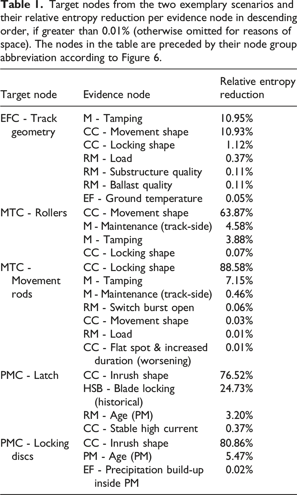
Considering such rankings for all target nodes, we found that the evidence nodes that play a role in the evaluation scenarios also consistently appear at the top of the respective rankings. Overall, the most important evidence group is dominantly the current curve features. Next are past maintenance actions and historical switch behavior, while railway meta data and environmental factors score lower. The power supply plays an important part in some scenarios, ruling out faults in the switch itself, but does not show significant importance in terms of relative entropy reduction. All in all, this assessment is in line with the expectations of the maintenance experts and indicates where maintenance operators should focus their information gathering and storage efforts.

On the downside, relative entropy reduction is difficult to grasp number wise. Furthermore, the different variants of the scenarios showed how powerful the combination of different evidence nodes can be for application in fault diagnosis. For instance, considering the target node track geometry in variant (b) of the first scenario, tamping together with other influencing factors shifted the model’s diagnosis from 41% roller maladjustment and 53% impaired track geometry to 4% roller maladjustment and 93% impaired track geometry. The entropy analysis highlights tamping, but the relative entropy reduction of all other influencing factors is between 0.3 and 0.1%. However, if we exclude tamping from the evidence set in variant (b), the model diagnosis is still 32% roller maladjustment and 64% impaired track geometry, i.e. a approximately 10% shift from the base scenario for both potential fault root causes in opposite directions, marking these influencing factors as valuable information in practice. Similarly, the evidence node precipitation build-up inside the point machine is at 0.02% for the target node locking discs, even though it is a relevant evidence in variant (a) of the second scenario. Thus, pairwise entropy analysis has limitations in assessing the effective (hidden) influences of some evidence nodes on the target nodes.

Analogously to the formulae above, the relative entropy reduction can also be calculated for sets of evidence nodes (and target nodes). As with the evaluation scenarios, a complete analysis of all (realistically possible) sets is not possible due to the exponential growth in the number of combinations that would have to be taken into account. Ultimately, analysis of entropy or other information theoretic measures can serve to provide comprehensive overviews of the connections between nodes in the model, and complementing the more application-driven scenario-based evaluation of the model.

Conclusions and outlook

This paper presents the development and evaluation of a Bayesian network diagnostic model that identifies fault root causes for railway switch point machines based on current curve features and various other sources of information. It covers the full range of faults (including rare events), is intuitive to maintenance operators and allows for automated integration into an operational workflow. The use of such a model during running operations frees up resources and would guarantee a certain standard in diagnosis, based on the combined knowledge of the experts involved in the modeling, regardless of their availability in day-to-day operations.

The development of Bayesian networks does not require an extensive database, and their reasoning process is traceable with directly human-interpretable outputs. Extensions to include more measurement data features or other information either based on expert knowledge or labeled data and continuous improvement are relatively easy to realize, compared to e.g., neural networks. On the downside, the model’s output given evidence, i.e., a ranking of the most likely causes of failure with associated probabilities, must be interpreted as strictly qualitative unless full data-based validation is performed. The development of a quantitatively reliable model would require a large amount of labeled data, even if only the parameters of the model are to be learned from data, while its structure is predetermined by expert knowledge. An early implementation of the presented (qualitative) model and a corresponding feedback loop from maintenance operators would significantly help to generate such a dataset in the long-term.

In the entropy analysis, the features derived from the current curve data proved to be the strongest evidence nodes. However, in the scenario-based evaluation, other sources of information can in some cases have a strong influence on the fault ranking provided by the model. By themselves, most of this information does not have a significant impact on the failure probabilities of the target nodes. Instead, they are often most effective when added to the current curve evidence, e.g., to narrow the diagnosis in case of several equally likely faults. Entropy analysis, which only considers pairwise influences, does not reveal these effects. For this reason, and because scenarios are closest to the practical application of such a model, scenario-based evaluation should be used primarily during the development process and approval of the model by experts.

Recalling the two example scenarios, the model’s traceability makes fault propagation tangible. In case of point machines, this is especially important for impaired track geometry (caused, for instance, by insufficient tamping or low quality track substructure) and persistent non-fatal faults, which both cause increasing maintenance efforts in the long-term. The incorporation of track health information and other data sources (e.g., point machine motor power or control current measurements) would further improve the diagnostic power of the model, allowing better differentiation between actual causes and symptoms, and improving the information base for optimal maintenance decisions and RAMS requirements.

The next major step is to integrate the model into an operational environment, i.e., automated, reliable engineering of human-interpretable features and automatic evidence setting (including the definition of thresholds). It would also be necessary to implement a consistent feedback loop on the performance of the model in practice to facilitate continuous improvement.

Footnotes

Declaration of conflicting interests

The author(s) declared no potential conflicts of interest with respect to the research, authorship, and/or publication of this article.

Funding

The authors disclosed receipt of the following financial support for the research, authorship, and publication of this article: This project has received funding from the Shift2Rail Joint Undertaking (JU) under grant agreement No 881574. The JU receives support from the European Union’s Horizon 2020 research and innovation programme and the Shift2Rail JU members other than the Union. This publication reflects only the author's view. The Shift2Rail Joint Undertaking is not responsible for any use that may be made of the information it contains.

ORCID iDs

Susanne Reetz

Thorsten Neumann

Appendix

Figure 9.

Examples for reasoning processes in Bayesian network: No evidence case (upper left), causal reasoning (upper right), diagnostic reasoning (lower left) and intercausal reasoning (lower right).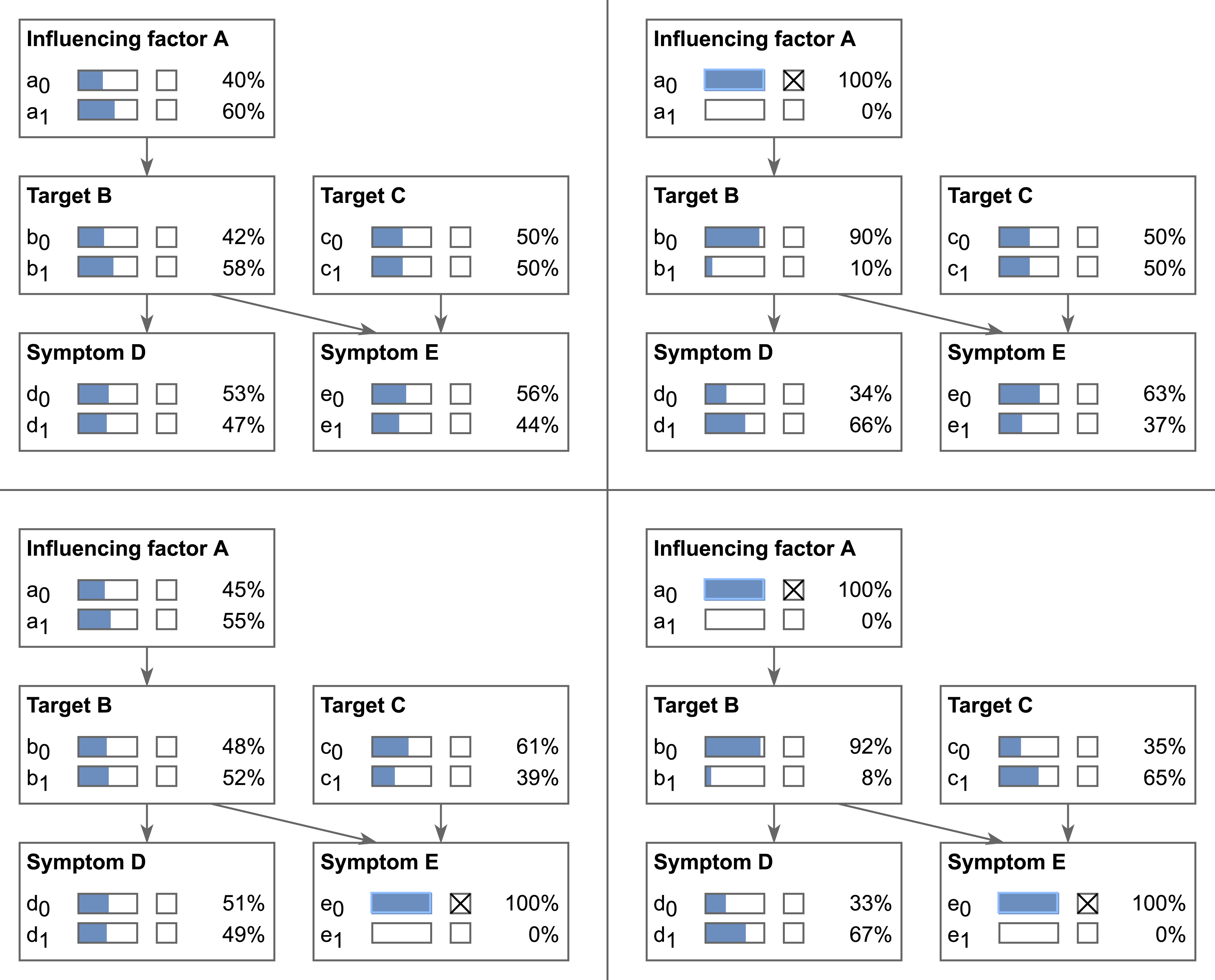

Bayesian networks are probabilistic graphical models that are able to mathematically represent complex statistical and/or causal relations between a number of random variables describing a system, for which knowledge may be incomplete. These models can be used to determine the most likely state of the system, model influences and infer causes from observed information. Common applications of Bayesian networks include medical diagnosis and decision support.

In a Bayesian network, random variables are represented as nodes with (discrete or continuous) states and relations between random variables as directed edges in an acyclic graph. Commonly, the directions of the edges follow causality. Nodes without edges between them are assumed to be independent in the sense that there is no direct influence (only potentially through other nodes). The exemplary Bayesian network in the upper left of Figure 9 has five nodes A − E (each with two discrete states) with causal relations between them.

The parameterization of a Bayesian network comprises conditional probability tables (CPTs) for all nodes with at least one parent node (i.e., child nodes) and a-priori distributions for all nodes without parent nodes (i.e., root nodes). A CPT for a child node X consists of probabilities

p (X = x ∣ Y_{1} = y_{1}, \dots, Y_{n} = y_{n})

for all states x of X and for all states y₁, …, y_n of the parent nodes Y₁, …, Y_n. The a-priori distribution of a root node Z is given by p(Z = z) for all states z of Z. These probabilities are sufficient to efficiently calculate the probabilities for all states of all nodes. From a mathematical point of view, the graph structure of a Bayesian network with its independence assumptions drastically reduces the (otherwise exponential) number of feasible joint probability distributions between all random variables. The CPTs and root probabilities uniquely determine which joint probability distribution the network has. Both structure and parameterization of a Bayesian network can be learned from data, whereas learning both requires a much larger amount of data than pre-specifying the structure and learning the parameterization only.

The strength of Bayesian networks is that once additional information on the modeled situation is available, it can be used to adapt the prediction of the model. If the current state of a node is known, this information is entered into the model as evidence to update the state probabilities in the remaining network accordingly. Technically, this is achieved by re-running the inference algorithm. If the model structure is based on causal relations, the model essentially mimics human logic to reason about the effects of new information. Consider the example network in Figure 9. Say the target nodes B and C are components of a technical asset whose health condition we aim to evaluate. The states b₀ and c₀ each represent faults, while b₁ and c₁ denote the healthy state of the respective component. The asset component B is dependent on the influencing factor node A. The asset state influences sensor data features, described by the symptom nodes D and E. The output of the model is a ranking of all fault states of all target nodes by descending probability given the current evidence, in this case b₀ and c₀. Multiple faults can occur simultaneously, so the probabilities of all fault states of all target nodes do not have to sum to one (i.e., fuzzy multi-label classification). The initial distribution without any evidence is shown on the upper left of the figure. In the upper right graphic, the model uses causal reasoning to determine the influence of the evidence that A is in state a₀ on its successive nodes B, D and E downstream in the network. Diagnostic reasoning in turn propagates information upstream. In the lower left graphic, information on the state of E changes the state probabilities of its predecessors C, B, and A. The changed probability distribution in B then again influences D. Combining causal and diagnostic reasoning into intercausal reasoning can lead to an effect called “explaining away”. In the example network, evidence of a₀ increases the probability of b₀ but does not change C, whereas evidence of e₀ increases the probabilities for b₀ and c₀ both. Given both evidences (i.e., a₀ and e₀) as in the lower right graphic, b₀ has an even higher probability, while the probability for c₀ drops. Thus, knowing a₀ to some extent eliminates c₀ as a potential cause for e₀.

All in all, the graphical, interpretable structure and traceable argumentation processes make Bayesian networks highly transparent models, in contrast to many other popular approaches in the field of expert systems and artificial intelligence.

References

Innovation in the spotlight: enhancing tracks, switches and crossings – the building blocks of rail. https://rail-research.europa.eu/news/innovation-in-the-spotlight-enhanced-track-systems/ (accessed 30 September 2022).

Swier

. Ways to improve the performance (and cost) of switches. In: Galeazzi

Kjartansson Danielsen

Kjær Ersbøll

, et al. (eds) Intelligent quality assessment of railway switches and crossings. Cham: Springer International Publishing, 2021, pp. 261–274.

Atamuradov

Medjaher

Dersin

, et al. Prognostics and health management for maintenance practitioners - review, implementation and tools evaluation. Int J Progn Health Manag 2017; 8(60): 1–31.

García Márquez

Lewis

Tobias

, et al. Life cycle costs for railway condition monitoring. Transp Res E Logist Transp Rev 2008; 44(6): 1175–1187.

Côme

Samé

Aknin

, et al. Anomaly detection in curve streams using the fisher score test: application to railway switch monitoring. In: Pombo

(ed) International Conference on Railway Technology 2012 (RAILWAYS 2012) . Civil-Comp Proceedings, Las Palmas de Gran Canaria, Spain: Civil-Comp Press, pp. 673–684.

Narezo Guzman

Hadzic

Groos

. Anomaly detection for railway switch monitoring data to enable condition-based maintenance. In: 12th World Congress on Railway Research, Tokyo, Japan, 28 October 2019.

Hamadache

Dutta

Olaby

, et al. On the fault detection and diagnosis of railway switch and crossing systems: An overview. Appl Sci 2019; 9(23): 5129.

Huang

Zhang

, et al. Turnout fault diagnosis through dynamic time warping and signal normalization. J Adv Transp 2017; 2017(2): 1–8.

Narges

Ahmad

Fereydoun

. A hybrid fault diagnosis scheme for railway point machines by motor current signal analysis. Proc Inst Mech Eng F J Rail Rapid Transit 2021; 236(9): 1026–1034.

10.

Guo

Wan

. An unsupervised fault-detection method for railway turnouts. IEEE Trans Instrum Meas 2020; 69(11): 8881–8901.

11.

Silmon

Roberts

. Improving railway switch system reliability with innovative condition monitoring algorithms. Proc Inst Mech Eng F J Rail Rapid Transit 2010; 224(4): 293–302.

12.

Pourret

Marcot

. Bayesian networks: a practical guide to applications. England: John Wiley & Sons, 2008.

13.

Weber

Medina-Oliva

Simon

, et al. Overview on Bayesian networks applications for dependability, risk analysis and maintenance areas. Eng Appl Artif Intell 2012; 25(4): 671–682.

14.

Cai

Huang

Xie

. Bayesian networks in fault diagnosis. IEEE Trans Ind Inf 2017; 13(5): 2227–2240.

15.

Charniak

. Bayesian networks without tears. AI Mag 1991; (4): 50–63.

16.

Koller

Friedman

. Probabilistic graphical models: principles and techniques. Adaptive computation and machine learning. Cambridge, Mass: MIT Press, 2009. ISBN: 9780262013192.

17.

Neumann

Narezo Guzman

. Bayesian network design for fault diagnostics of railway switches. In: Beer

Zio

(eds) 29th European Safety and Reliability Conference: ESREL 2019 Singapore: Research Publishing Services, pp. 1117–1124.

18.

Beer M and Zio E (eds) 29th European Safety and Reliability Conference: ESREL 2019. Singapore: Research Publishing Services, 2019 . ISBN 978-2-8322-5915-3. https://www.vde-verlag.de/iec-normen/225834/iec-60812-2018.html

19.

Narezo Guzman

Heusel

Weik

, et al. Towards the automation of anomaly detection and integrated fault identification for railway switches in a real operational environment. In: World Congress on Railway Research 2022.

20.

Bemment

Goodall

Dixon

, et al. Improving the reliability and availability of railway track switching by analysing historical failure data and introducing functionally redundant subsystems. Proc Inst Mech Eng F J Rail Rapid Transit 2017; 232(5): 1407–1424.

21.

Rama

Andrews

. A reliability analysis of railway switches. Proc Inst Mech Eng F J Rail Rapid Transit 2013; 227(4): 344–363.

22.

Hassankiadeh

. Failure analysis of railway switches and crossings for the purpose of preventive maintenance.

23.

Kassa

. Analysis of failures within switches and crossings using failure modes and effects analyisis methodology. In: Proceedings Intelliswitch Symposium, Copenhagen, Denmark.

24.

voestalpine WBN . Voestalpine wbn wisselsteller type nse: installatie en onderhoudsvoorschrift.

25.

Zagorecki

Druzdzel

. Knowledge engineering for bayesian networks: how common are noisy-max distributions in practice? IEEE Trans Syst Man Cybern Syst 2013; 43(1): 186–195.

26.

BayesServer . Relevance tree inference. https://www.bayesserver.com/api/dotnet/api/BayesServer.Inference.RelevanceTree.RelevanceTreeInference.html, (accessed 22 August 2022).

27.

Cover

Thomas

. Elements of information theory. 2nd ed. Hoboken, New Jersey: John Wiley & Sons, Inc., 2006.

Expert system based fault diagnosis for railway point machines

Abstract

Keywords

Introduction

Information sources

Historical data

Experimental data

Expert knowledge and other sources

Development process

Structural design

Temporal scope

Parameterization

Scenario-based evaluation

Model and exemplary scenarios

Model

Exemplary scenarios

Entropy analysis

Conclusions and outlook

Footnotes

Declaration of conflicting interests

Funding

ORCID iDs

Appendix

References