Sage Journals: Discover world-class research

Abstract

A simulation framework for three-dimensional particle trajectory tracking, snow accumulation and ice accretion modelling on solid bodies in high-speed air flow is presented. The framework, named HADICE, solves the aerodynamic flow field as Reynolds averaged Navier-Stokes (RANS), with optional hybrid RANS/LES capabilities for modelling complex turbulent flows. Particle trajectory tracking is performed in an Eulerian-Lagrangian approach and wall collision is modelled using a hard collision model with reflect condition and a momentum based trap condition. A novel accurate and robust iterative evaluation method for the local collection efficiency is proposed for arbitrary 3D geometry and flow. Ice accretion is modelled in a multi-step approach and iced geometry is updated through mesh deformation using a radial basis function (RBF) interpolation method. Snow accumulation and ice accretion predictions based on the framework are validated against climatic wind tunnel experimental measurements. A full 3D simulation is demonstrated for snow accumulation and ice accretion on a 1:8 scaled high-speed train model. Using the presented framework, snow accumulation and icing simulation for high-speed trains can be conducted in an accurate and efficient manner, which is of great importance for physical investigations and the design of anti-snow and ice protection systems.

Keywords

Computational fluid dynamics particle trajectory tracking snow accumulation icing high-speed train

Introduction

Background and motivation

As the business of high-speed train expands to more regions around the world, variation in environmental conditions must be taken into account during the design of trains. When operating in extremely cold rainy and snowy weather, water droplets and snow can accumulate on the outer surface of the train body including critical areas such as the bogie and pantograph. Due to heat generation by internal components (such as motors, brakes and gears), the accumulated snow can melt and freeze as ice. Snow accumulation and ice accretion pose serious concern on the control and safety of high-speed train operation, which must be considered during design.

Understanding the dynamics of multiphase flow and ice accretion is of critical engineering and scientific importance. Mathematical solution of multiphase flow is notoriously difficult, therefore exact analytical solutions only exist for fundamental problems such as the steady state and quasi-steady movement of bubbles and droplets in Stokes flow. Experimental investigations of multiphase flows are complex and costly. Full-scale testing is possible in some cases, however in many situations scaled models must be used (for instance train carriages) and simplifications in testing conditions must be taken. As a result, computational models are becoming favourable for physical understanding as well as aiding the design process.

Computational simulation of the motion of snow particles or water droplets in air requires modelling for the air flow and the particle phase. There are two main approaches for modelling the particle field. One approach is to follow individual particles or particle trajectories, this is the Lagrangian approach. Another approach is to treat the particles as a cloud with continuum-like behaviours, this is the Eulerian approach. Together with the model for the background flow (which is usually treated in the Eulerian approach), these two approaches are commonly known as Eulerian-Lagrangian and Eulerian-Eulerian approaches respectively.¹ Both approaches have seen application in various open-source codes (e.g., OpenFOAM) and proprietary computational software (e.g., Ansys Fluent); they are used in a number of researches to study snow accumulation on object surfaces.^2–12

Over the past decades, a number of computational models for predicting ice accretion have been developed. The classical approach to ice-accretion prediction is introduced by Messinger,¹³ which provides the theoretical basis for the majority of state-of-the-art icing models. Examples of icing solver include LEWICE,¹⁴ MULTI-ICE,¹⁵ FENSAP-ICE¹⁶ and PoliMIce.¹⁷ One of the key challenges for icing simulation in the Eulerian-Lagrangian multiphase approach is the calculation of the local collection efficiency, which describes the ratio of the particle flux at the impingement location to the particle flux in the free stream. Determining the local collection efficiency is a prerequisite for solving the conservation of mass in ice accretion problems. LEWICE3D.¹⁸ calculates the ratio of the termination area to the free stream area of a flux tube, whose cross-section is rectangular defined by four adjacent trajectories. This method is designed for wing-like geometries where flow remains largely two-dimensional. It is likely to under-perform, if not fail, when strong 3D flow recirculation is present causing the crossing and topology change of flux tubes. A variation of the LEWICE3D method was proposed by Xie et al,¹⁹ which utilises adaptive trajectory mesh refinement and interpolation and showed success on multi-element wings. Similar success was achieved by Wright et al.²⁰ using an automated refinement algorithm in GlennICE for wings and engine intake.

Recent studies on snow accumulation on trains.^2–12 were all conducted using commercial software Ansys Fluent using the Eulerian-Lagrangian approach with the discrete phase model (DPM). In all the work, only the snow particle accumulation is simulated and icing is not modelled. Most simulations were based on unsteady Raynolds-averaged Navier-Stokes (URANS) with k-ϵ realisable turbulence model, with a couple of exceptions using the hybrid RANS/LES methods of DES and IDDES. Very limited qualitative comparisons were made with experimental observations. Computational models used in past research vary from scaled bogie with simplified train body to full train set with multiple carriages. The model size for these studies ranges between 20 and 40 million grid cells, which were shown to be sufficient for bogie-only simulation. However, for large-scale simulations with full train set, grid size requirement is expected to increase considerably to capture the complex flow behaviour. High-fidelity computational simulation of snow accumulation and ice accretion is a new and emerging subject, which requires continuous research and update of numerical tools. Therefore, there is a necessity for developing a simulation framework that can accurately and efficiently simulate air flow, snow accumulation and ice accretion on high-speed trains.

Objectives

High-fidelity computational simulation will play a leading role in multiphase flow research and application in the coming decades. Currently, during the research and development of high-speed trains, industrial standard preliminary studies on snow accumulation, ice accretion and anti-icing performance rely heavily on empirical knowledge and testing. In the case where computational modelling is conducted, the calculation methods used are generally relatively simple and cannot support complex analysis of snow accumulation and icing at critical areas in an efficient and robust manner, which makes effective anti-snow and anti-icing designs challenging.

The main objective of this work is to develop an accurate and efficient computational simulation framework for modelling wind-snow two-phase flow and icing for high-speed trains. The framework is capable of predicting fluid dynamic behaviours in various environmental conditions such as snowfall, snow suspension and the related thermodynamic phenomena such as icing and melting. This paper presents the development and validation of the simulation framework.

It should be noted that the main focus for train icing differs from that for aircraft icing. The micro-scale prediction of exact geometry change, especially near the leading edge, is of utmost importance for lifting devices such as wings and rotor blades. For train icing, the main interest is in the macro-scale spatial deposition and total accumulated mass, which are used to guide anti-icing designs. The main areas of icing, based on field operation experiences, are in the bogie and pantograph regions, which have negligible impact on the drag compared with the train body itself. Therefore, the main challenge for this work lies in the computational challenge to accommodate large-scale ice accretion in complex separated flows around three dimensional convex and concave bodies.

Simulation framework and methodology

Overview of framework

Particle motion and ice accretion are unsteady by nature. Ice buildup on a surface depends on the conditions of surrounding air flow and the incoming mass flux (snow particles or supercooled water droplets). Over time, the accumulated ice alters the surface shape and changes the surrounding air flow. Large variation of local flow field results in changes in particle trajectories and consequently the collected mass, which eventually modifies the ice accretion. Therefore, accurate simulation of ice accretion must include capabilities to capture all the aforementioned phenomena.

The proposed simulation framework, named HADICE, is illustrated in Figure 1. The core solver consists the following main modules: a Navier-Stokes solver for modelling the continuous fluid phase (i.e., air flow), a particle tracking module to capture trajectories using the Eulerian-Lagrangian approach, an icing module for calculating ice thickness and a mesh deformation module for obtaining the iced geometry. At start, aerodynamic flow field is computed based on the user input fluid domain mesh (clean surface) and boundary conditions. Next, particles are seeded into the computation domain and their trajectories are modelled until impingement on the surface. Using mass and thermal balances on the surface, accreted ice can be simulated over a given time period. After obtaining the ice shape, the surface geometries are updated and the volume mesh of the fluid domain is deformed accordingly. Subsequently, aerodynamic flow modelling is conducted again for the new geometry and the whole process repeats until total simulation time is reached. In combination, these modules can model air flow past an object, particle trajectory and accumulation, ice accretion and the resultant iced geometry.

Figure 1.

Overview of the simulation framework.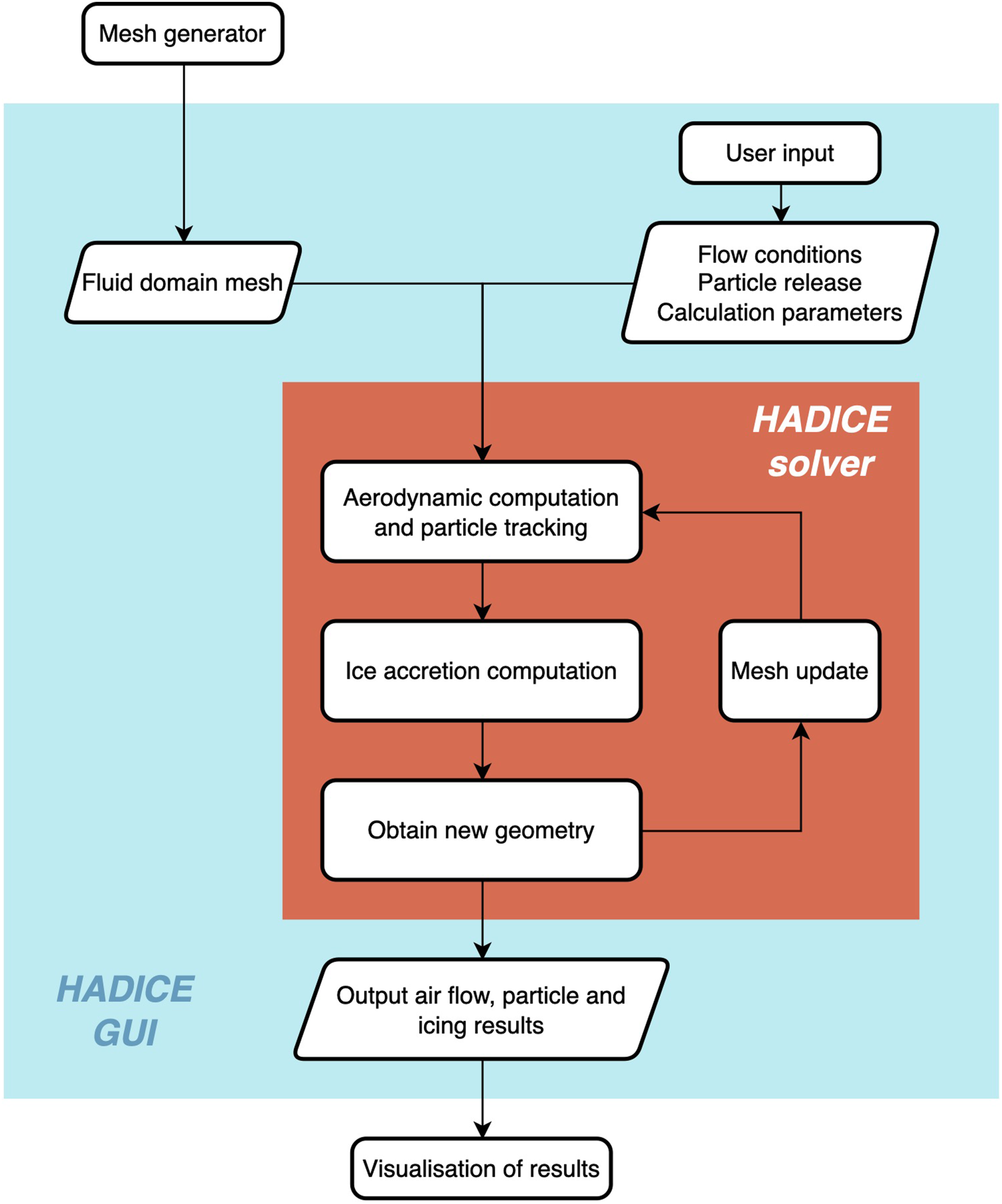

The programming was carried out using Fortran 2018 and parallelisation is achieved through the Message Passing Interface (MPI).²¹ using CPU cores. Code execution is performed in the command line interface (CLI) on workstation and HPC; a graphical user interface (GUI) is also available.

The following sections describe the key numerical methods used in the code.

Aerodynamic flow solver

The aerodynamic flow solution is calulated using the in-house flow solver HADES, which is a 3D, time-accurate, compressible, viscous, finite volume, hybrid RANS/LES flow solver for unstructured meshes. The flow variables are represented on the nodes of a generic unstructured grid and numerical fluxes are computed along the edges of the grid. The numerical fluxes are evaluated using Roe’s flux vector difference splitting.²² to provide matrix artificial dissipation in a Jameson-Schmidt-Turkel (JST) scheme.²³ The solver is based on the one-equation Spalart-Allmaras turbulence model.²⁴ Standard wall function²⁵ is used at viscous wall boundaries. The overall solution method is implicit, with second-order accuracy in space and time. For steady-state flow computations, the solution is advanced in pseudo-time using local time stepping and solution acceleration techniques such as residual smoothing; while dual time stepping is used for time-accurate unsteady computations. Unsteady flow computation can be computed using unsteady Reynolds-averaged Navier-Stokes (URANS) or Delayed Detached Eddy Simulation (DDES).²⁶

Validation and verification of HADES in various 2D canonical flows and high-speed 3D compressible applications can be found in past publications.^26,27

Particle trajectory tracking

Particle trajectory tracking is carried out based on the Eulerian-Lagrangian approach. This method allows explicit tracking of particle trajectories and is referred to as the discrete element method (DEM) in the literature. This type of method has been used by a number of researchers in recent years for studying snow accumulation on high-speed trains.^2–10 Figure 2 shows the flow chart illustrating the key steps in the particle trajectory tracking operation. Detailed information of the algorithm is given in the following.

Figure 2.

Flow chart illustration for the particle trajectory tracking algorithm.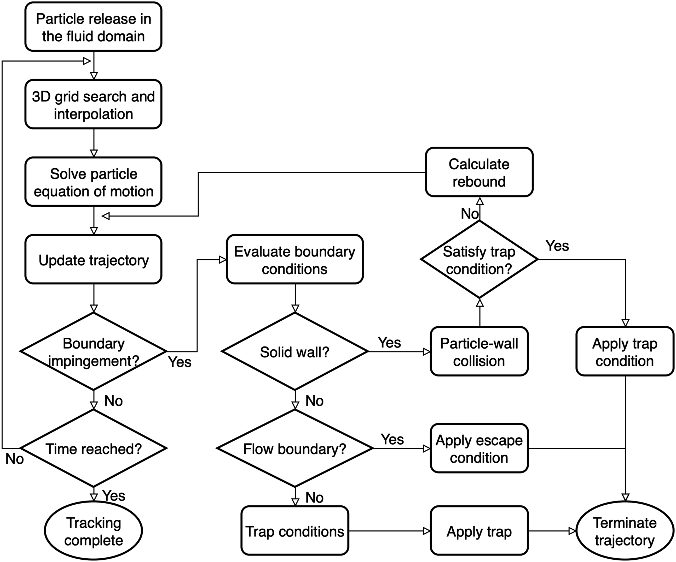

Particle equation of motion The general dynamic equation for a particle can be written as follows

\frac{d v_{p}}{d t} = \frac{18 μ_{f}}{ρ_{p} d_{p}^{2}} \frac{C_{d} {R e}_{p}}{24} (u_{f} - v_{p}) + \frac{ρ_{p} - ρ_{f}}{ρ_{p}} g

(1)

where v_p is the velocity of the particle at the centroid, u_f is the local fluid velocity vector and t is the time. The first term on the right hand side represents the aerodynamic drag force per unit mass, where ρ_p is the particle density, d_p is the particle diameter, μ_f is the dynamic viscosity of the fluid, C_d is the drag coefficient, Re_p is the relative Reynolds number which characterises the relative motion between the particle and the fluid. The second term on the right hand side represents the combined gravitational and buoyancy forces per unit mass, where g is the gravitational vector and ρ_f is the fluid density. Other forces such as Basset history force, Saffman lift force, particle collision and particle rotation are not considered.

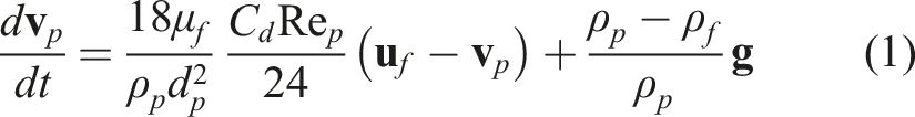
The above equation can be coupled with the equation for particle trajectory

\frac{d x_{p}}{d t} = v_{p}

(2)

where x_p denotes the instantaneous location of particle.

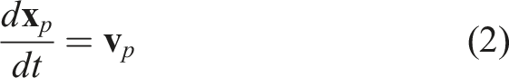
The above equations governing the particle velocity and trajectory are a set of coupled ordinary differential equations (ODEs) and can be solved through numerical integration with temporal discretisation of physical time step.

Efficient trajectory pathing in 3D unstructured mesh The solution of particle equation of motion requires explicit tracking of particle trajectories in the fluid domain. Since instantaneous particle location is not guaranteed to coincide with the fluid mesh vertices (where the Navier-Stokes solver data is saved), searching for the mesh cell enclosing the particle and interpolation are required. Locating the mesh cells for particle seeds can be performed in a straightforward manner during pre-processing. As particles move across mesh cells, a new residing cell needs to be found on the fly. To accomplish this, a search algorithm for an arbitrary 3D unstructured mesh is developed. The method uses a directional search algorithm based on the intersection between the instantaneous particle velocity vector and the cell boundaries. This method is directional and computationally efficient. Considering that in real cases, particles usually do not travel large distances within each physical time step, the next residing cell is likely to be adjacent to the previous residing cell, resulting in minimal search cost.

Particle-wall collision Broadly speaking, the outcome of particle-wall collision can be categorise into three types: escape, reflect and trap. The escape condition terminates particle trajectory and removes the particle from the computation domain. The reflect condition evaluates the collision between particle and wall and determines the state of the particle after collision, i.e., velocity vector after rebound. The reflect condition is usually coupled with a trap criterion (see Figure 2), which evaluates whether the particles will rebound from the surface or remain stationary on the surface. In computational simulations, reflect conditions are applied at the surfaces where accumulation is to be simulated.

In the current model, particle-wall interaction is treated as a single spherical particle without rotation colliding with a solid wall. The energy loss during collision is treated using the hard sphere model with coefficients of restitution. The particle velocity after a wall collision can be derived from the impulsive equations,²⁸ based on which two types of collisions are classified:

• A collision without sliding takes place when

| \frac{v_{t}^{i n}}{v_{n}^{i n}} | \leq \frac{7}{2} μ_{0} (1 + e_{n})

(3)

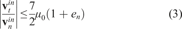
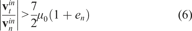
The corresponding velocity components after collision are calculated by

\begin{array}{c} v_{n}^{o u t} = - e_{n} v_{n}^{i n} \end{array}

(4)

\begin{array}{c} v_{t}^{o u t} = \frac{5}{7} v_{t}^{i n} \end{array}

(5)

• A sliding collision takes place when

| \frac{v_{t}^{i n}}{v_{n}^{i n}} | > \frac{7}{2} μ_{0} (1 + e_{n})

(6)

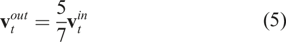
The corresponding velocity components after collision are calculated by

\begin{array}{c} v_{n}^{o u t} = - e_{n} v_{n}^{i n} \end{array}

(7)

\begin{array}{c} v_{t}^{o u t} = v_{t}^{i n} - μ_{d} (1 + e_{n}) v_{n}^{i n} \end{array}

(8)

In the above equations, e_n denotes the normal coefficient of restitution, μ₀ is the static coefficient of friction, μ_d is the dynamic coefficient of friction, superscripts in and out denote incident and rebound velocities, subscripts n and t denote components normal and tangential to the wall respectively. The velocity components satisfy v = v_n + v_t. By default, the static and dynamic friction coefficients are taken as as μ₀ = 0.4 and μ_d = 0.3 respectively;²⁹ re-calibration of these coefficients are likely needed for specific application, which can be done by comparison with experimental measurements.

The coefficient of restitution usually takes an empirical value which strongly depends on the particle velocity, the collision angle and the material properties of the particle and the wall. For irregular bouncing of particles due to wall roughness, the model based on Sommerfeld.²⁹ is used. In the case of snow particles, the coefficient of restitution is usually unknown and highly dependent on the properties of the snow and the wall surface. Therefore, a general form of post-collision velocities is also included as an option in the model with $v_{t}^{o u t} = e_{t} v_{t}^{i n}$ , where e_t represents the tangential coefficient of restitution accounting for the momentum loss. The model form for the normal velocity component follows the usual way (Equation (7)).

The collision between particle and wall can also result in no rebound. The trap condition terminates particle trajectory and brings the particles to rest at the point of contact. The trapping of particles is due to the resultant balance between wall friction and the aerodynamic forces. The model for the physical trap condition is based on the nature of particle saltation and suspension. In Bagnold’s classical definition of particle transportation modes,³⁰ two wind velocity thresholds are introduced: the impact threshold, which is the wind velocity that must be exceeded for particle saltation to be sustained, and the fluid threshold, which must be exceeded for saltation to be initiated. Since the fluid threshold velocity is generally greater than the impact threshold velocity,³¹ the fluid threshold velocity from Bagnold’s formula³⁰ is used for the physical trap condition. For snow particles, this value is given as 0.21m/s. In practice, the fluid threshold velocity is sometimes used together with a threshold incident angle α_crit³² as physical trap criteria; in this study, the threshold incident angle is taken as 45°.

Calculation of accumulation mass

Obtaining the mass of accumulated particles is a prerequisite for solving the ice accretion problems. The state-of-the-art methods for evaluating accumulation mass can be broadly categorised into two approaches: (1) direct unsteady simulation; (2) quasi-steady approximation. The direct unsteady simulation approach is quite straightforward. A finite number of particles are injected into the computational domain and their movements are tracked numerically in a time-accurate fashion. This can be achieved by performing unsteady computations for the fluid phase using URANS or DES. Another approach of evaluating the accumulation mass is based on the quasi-steady assumption. In this approach, particle accumulation is modelled by taking the mean flow as steady and without large fluctuations in the trajectory path. The distribution of accumulated mass is calculated from a so-called local collection efficiency.¹⁴ The local collection efficiency β represents the ratio of the particle mass flux at the impingement location to the particle mass flux in the free stream (usually at the injection). Using the computed local collection efficiency, the accumulation mass flux (kg/m²s) on the surface of interest can be directly calculated from the known mass flux at the injection plane. The key assumption in this approach is that particle trajectories do not oscillate significantly in time, based on which a time-independent local collection efficiency can be approximated.

The main advantage of the direct unsteady simulation approach is the preciseness in the tracking of each injected particle (or parcel), which is particularly useful when the injected particles have various properties and non-uniform spatial distribution. On the contrary, the local collection efficiency approach in practice generally requires particles to be uniformly spaced when injected into the free stream. Moreover, the time-accurate modelling approach may be necessary when the fluid in the particle path experiences large amplitude fluctuations, which invalidates the calculation of local collection efficiency. The major limitation of the direct unsteady simulation approach is its high computational cost, which increases with the amount of injected particles, the time duration to be simulated as well as the unsteadiness in the flow. As a result, the local collection efficiency approach is widely adopted for ice accretion computations where minutes or even hours of physical time duration need to be simulated, whereas the typical simulation time using the direct unsteady simulation approach is limited to 1-5 seconds.^3–10

In the developed framework, both approaches are implemented. The direct unsteady simulation method is used to study the behaviour of snow particle movement and the physics of accumulation; the fluid phase can be solved either steady or unsteady. Ice accretion is modelled based on the quasi-steady approach using a frozen (time-averaged) flow solution and a time-accurate icing solver; the result is an approximation to the averaged ice shape. The quasi-steady icing simulation is capable of capturing the major icing areas, while neglecting areas with very low amount of accumulation due to flow unsteadiness; it is considered good tradeoff for engineering applications.

For the ice accretion model, additional computation is required to compute the local collection efficiency, which is explained below.

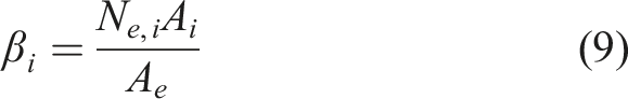
The definition of local collection efficiency in three-dimensional space is given by β = dA_i/dA_s, where A_i denotes the cross-sectional area of the flux tube in the free stream (e.g., spacing at the injection plane) and A_s is the termination area of the flux tube on the impingement surface.¹⁸ For general 3D geometries and flows, the preservation of flux tube topology until impingement is not guaranteed. Therefore, direct calculation of flux tube area ratio at termination to that in the free stream as demonstrated in LEWICE3D¹⁸ can lead to erroneous results. To address this issue, a new iterative method based on statistical approximation is proposed. Instead of calculating the area ratio explicitly, the local collection efficiency is evaluated from the ratio of particle frequency at the impingement surface to the particle frequency at the seeding plane in the free stream. The detailed process is explained below.

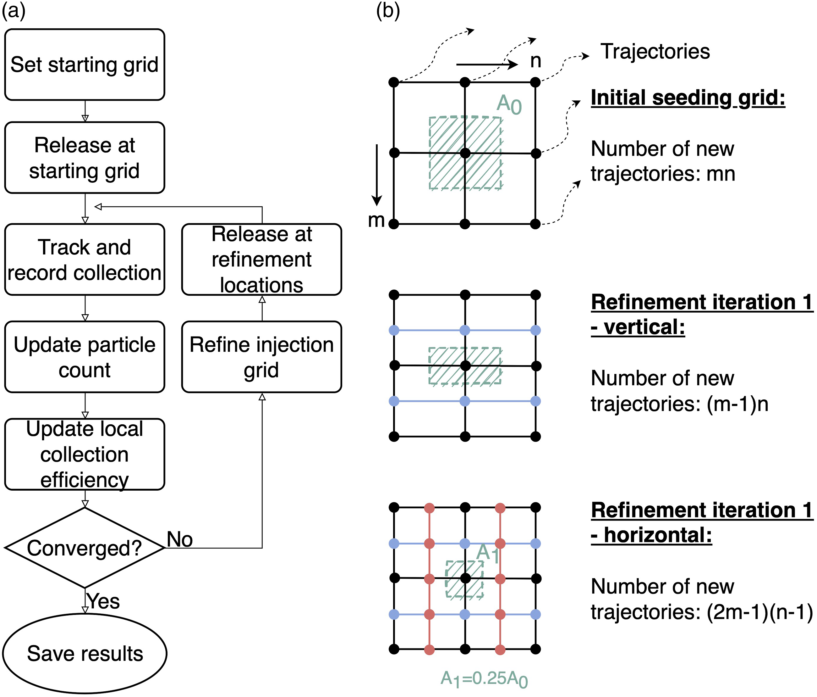
Figure 3(a) shows the flow chart for calculating the local collection efficiency through iterative refinement of the seeding grid and Figure 3(b) illustrates the setup for the seeding grid in the free stream and its refinement strategy. The calculation steps are explained as follows (see Figure 3(b) for an example):

(1) Define a rectangular seeding plane upstream of the surface of interest.

(2) Set a regular seeding grid with m × n uniformly spaced release points. The area spacing in the free stream A_i is saved (i = 0 for the initial seeding grid).

(3) Release particles at the seeding grid vertices and trace their trajectories in the fluid domain until wall collision. Record the number of trapped particles on the object surface.

(4) On the object surface, go through each of the 2D mesh elements and calculate the element-wise local collection efficiency as

β_{i} = \frac{N_{e, i} A_{i}}{A_{e}}

(9)

where N_e,i denotes the total number of trajectories terminated in this mesh element, A_e denotes the area of the mesh element and i denotes the refinement iteration index for the free stream seeding grid.

(5) Compute the mean and max residuals of the local collection coefficient over the surface mesh using

R (β) = {\begin{array}{c} β_{i}, & i = 0 \\ β_{i} - β_{i - 1}, & i > 0 \end{array}

(10)

(6) Assess the convergence criteria for residuals. If not converged, refine the seeding grid horizontally and vertically at the mid-points of the existing grid structure (as demonstrated in Figure 3(b)).

(7) Release particles at the newly added refinement locations and trace their trajectories until wall impingement.

(8) Update the frequency distribution of trajectories terminated on the surface mesh and recalculate β using equation (9) with the updated count N_e,i and seeding grid area spacing A_i.

(9) Compute and assess the residuals using equation (10). Repeat the refinement process until convergence is reached.

Figure 3.

(a) Flow chart for local collection efficiency calculation; (b) Refinement illustration for a 3 × 3 initial seeding grid.

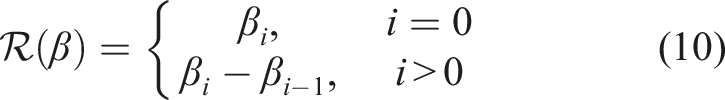
The value of the local collection efficiency residual directly relates to the physical resolution of the mass flux, for instance, a mean residual of 10⁻³ denotes the mass flux on the surface is resolved with a mean error equal to 0.1% of the injection mass flux. Therefore, the convergence criteria can be set based on the desired physical resolution level. To filter out high frequency noise and accelerate convergence, residual smoothing is performed at each refinement iteration based on the Laplacian of the surface mesh.

The above approach is novel and provides a generic method for accurate and efficient evaluation of the local collection efficiency for arbitrary 3D geometry and flow. This method takes advantage of the simplicity of direct unsteady simulation approach, which records the area density of accumulated particles on the surface for one shot of injected particles. Simultaneously, explicit tracking of the variation in flux tube cross-sectional area is not required and the estimation error can be reduced by discretisation of the injection grid.

Ice accretion model

The most widely used ice accretion model was originally proposed by Messinger.¹³ The Messinger model in its original form is a one-dimensional energy balance for an insulated, unheated surface exposed to icing. This model was later extended by Myers.³³ for aircraft icing; the current study follows this method. The formulation of the problem is based on the standard method of specifying a phase change, known as the Stefan problem.³⁴ Stefan problems are used extensively in the investigation of melting and solidification.

The typical problem formulation for icing is explained in the following. An ice layer of thickness B covers the solid substrate. For the case of glaze ice, a water layer of thickness h will also be present over the ice. The temperature in the ice and water is denoted by T and θ respectively. Due to the unsteady nature of the problem, all the aforementioned quantities are functions of time; temperature profiles are allowed in the normal direction to the surface.

The governing equations following the Stefan problem are given as follows

ρ_{i} \frac{\partial B}{\partial t} + ρ_{w} \frac{\partial h}{\partial t} = β U G

(11)

\frac{\partial T}{\partial t} = \frac{κ_{i}}{ρ_{i} c_{i}} \frac{\partial^{2} T}{\partial z^{2}}

(12)

\frac{\partial θ}{\partial t} = \frac{κ_{w}}{ρ_{w} c_{w}} \frac{\partial^{2} θ}{\partial z^{2}}

(13)

ρ_{i} L_{F} \frac{\partial B}{\partial t} = κ_{i} \frac{\partial T}{\partial z} - κ_{w} \frac{\partial θ}{\partial z}

(14)

where subscripts i and w denote ice and water respectively, ρ denotes density, β denotes local collection efficiency, U denotes freestream fluid velocity, G denotes liquid water content, κ denotes thermal conductivity, c denotes specific heat and L_F denotes latent heat of fusion from water into ice. The ice density ρ_i takes different values for rime or glaze ice, which are denoted ρ_r and ρ_g respectively. The transition between the two ice forms is assumed to be instantaneous.

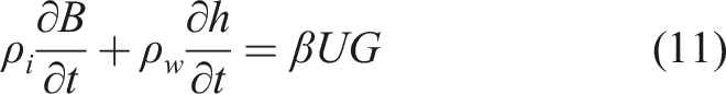
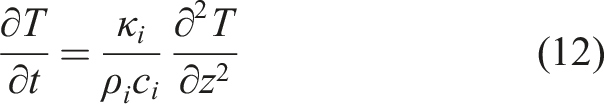
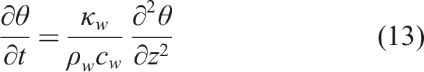
Equations (11)–(14) describe mass conservation, one-dimensional heat transfer in the ice and water, and the Stefan condition for ice fusion respectively. Several assumptions are made: the ice is assumed in perfect thermal contact with the substrate, the temperature is continuous at the phase change boundary which equals to the freezing temperature, and the temperature profile in the ice layer is assumed to be linear. Together with appropriate initial and boundary conditions, the four equations can be solved to obtain the ice and water thicknesses and their temperatures.

3D mesh deformation

Mesh adaptation or deformation of the fluid domain is necessary for modelling the iced geometry. Complete regeneration of the volume mesh is prohibitively expensive and can cause undesirable changes to the aerodynamic flow solution, leading to oscillation and uncertainty in computation predictions. Deformation of the existing volume mesh is more cost effective when geometries are updated frequently. An efficient RBF interpolation based algorithm is implemented. The method is developed based on,³⁵ which accurately captures global and local motions using all the surface points at significantly reduced cost compared to conventional full RBF methods.

Simulation predictions and comparison with experiment

In the next step, the capability of the developed simulation framework for predicting snow and ice accumulation on train is demonstrated. In order to validate the simulation predictions, an experimental campaign was conducted using geometries with varying complexity. In the following sections, the setup of experimental test, computational model and comparison between simulation and experimental results are presented.

Experimental test

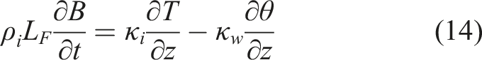
The wind tunnel test was conducted in the CAERI climatic wind tunnel (CWT) in Chongqing, China. The wind tunnel was designed by WBI Germany with capability for rain and snow generation, and has been conducting routine experiments on automobiles. The wind tunnel test section dimensions are 18m ×13m ×8m with max wind speed up to 200km/h and air temperature range between −10°C and −40°C. The snow generation nozzle can allow maximum flow rate up to 2400 L/h. A plane view of the wind tunnel test section is shown in Figure 4, where the placements of the snow generator and the test object are illustrated.

Figure 4.

Wind tunnel test section layout.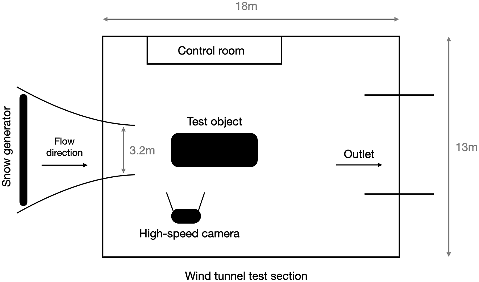

The first series of test was conducted using wall-hanging simple 3D prism objects. Figure 5 illustrates the geometry of the prism objects and their installation in the wind tunnel. The prisms are hung on a horizontal wooden plate mounted on the work bench. The motivation of testing simple prism objects is to gain knowledge on the particle accumulation physics and improve the numerical models. Moreover, the experimental measurements can be used as quantitative validation data for computational simulation. In this paper, results for three prism objects are presented. The geometry of the three prisms are identical with outline dimensions 20cm × 15cm × 10cm; all of them have a rectangular cut-out at one of the corners. Prisms 1 and 3 are rotated by 30°relative to the incoming flow in opposite directions away from the centre prism; this allows the investigation of effects such as flow separation and wall collision on particle accumulation. In the experiment, the wind-facing front surfaces are heated, so that snow can be melted to allow ice formation.

Figure 5.

Geometry and experimental setup for the simple 3D prism objects.

The second test is a 1:8 scaled high-speed train model with simplified geometries, as shown in Figure 6(a). The dimensions of the train model are 3.5 m in length, 0.4 m in width and 0.5 m in height. The model train consists of the front section of a head car, a short mid section representative of a passenger car and the rear section of a tail car. Two bogies and a pantograph with simplified geometries are also included (Figure 6(b)). The bogie is simplified from the real geometry and is symmetric about the centre plane. The underbody clearance between the train and the ground is representative of track operation. Figure 6(c) illustrates the installed train model in the wind tunnel, where the train was placed on top of a track.

Figure 6.

(a) Geometry of the 1:8 scaled train model; (b) Geometry of the simplified bogie; (c) Experimental setup for the simplified train model.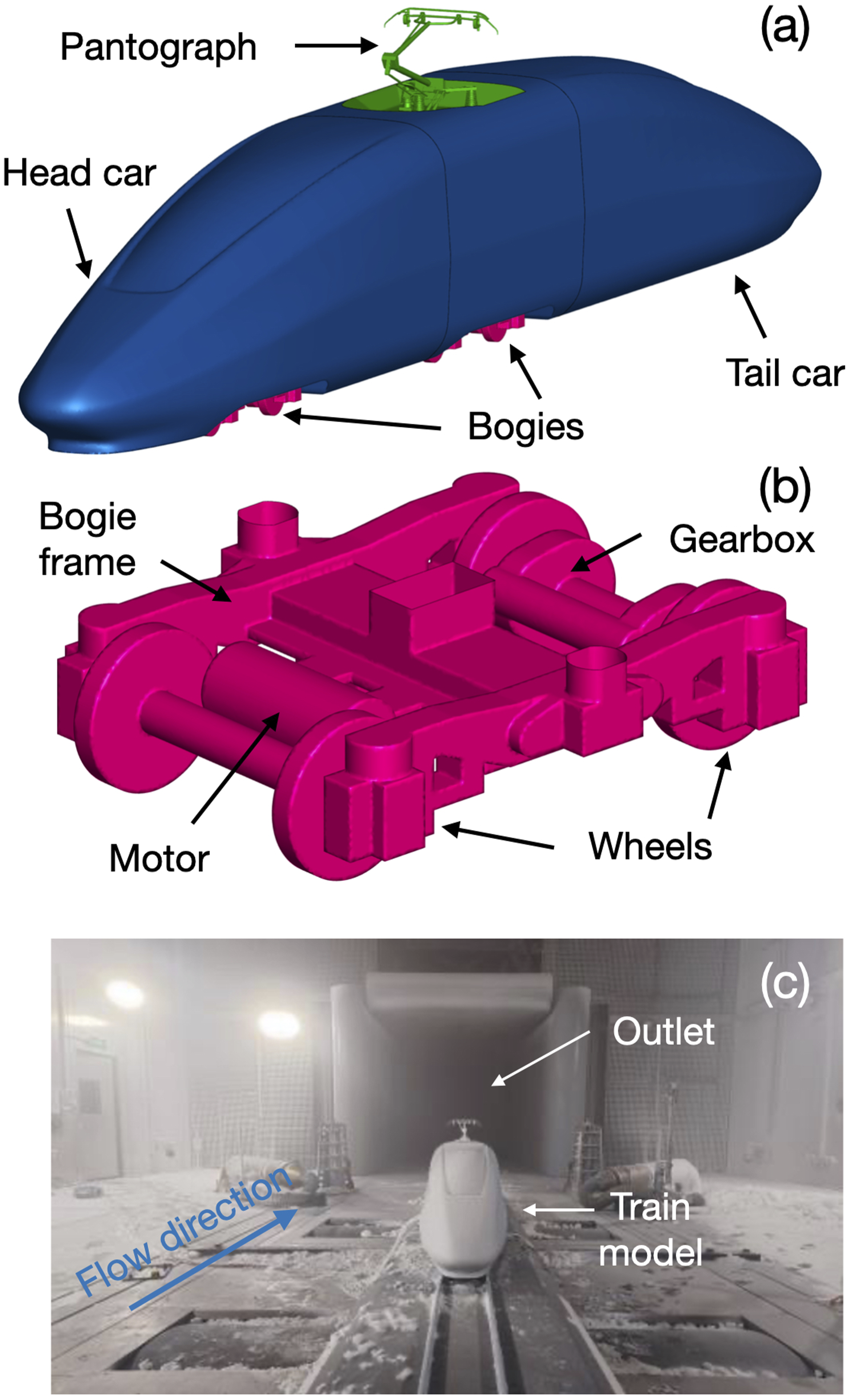

In the current work, the test condition corresponding to wind speed 25 m/s and ambient temperature −25°C is presented. In the experiment, the released snow particles are monitored by the OTT Parsivel2 laser precipitation disdrometer, which captures the size and speed of particles. The snow particles generated in the wind tunnel test were recorded with diameter varying in the range of 0.2–1.8 mm and injection spacial density of approximately 10g/m³.

It should be noted that climatic wind tunnel test with snow is challenging in practice, in that the characteristics of the generated snow particles cannot be precisely controlled. Moreover, uniform inlet conditions with particles are much harder to achieve than traditional aerodynamic experiments. These increase the difficulties for comparison with computational simulation. Therefore, discrepancies between experimental findings and simulation results are discussed and reviewed on a case-by-case basis.

Computational model

Figure 7(a) shows the computational domain and boundary conditions. The dimensions of the computational domain are the same as the wind tunnel test section. The test object is placed at the same position as tested in experiment, which is on the centreline of the wind tunnel. For the boundary conditions, the surfaces of the train body (including bogie, wheel and pantograph) and the ground are modelled as viscous walls using wall function. Riemann boundary conditions are used at the far-field flow boundaries with uniform 25 m/s free stream velocity and −25°C ambient temperature.

Figure 7.

(a) Computational domain; (b) Train surface mesh; (c) Bogie surface mesh.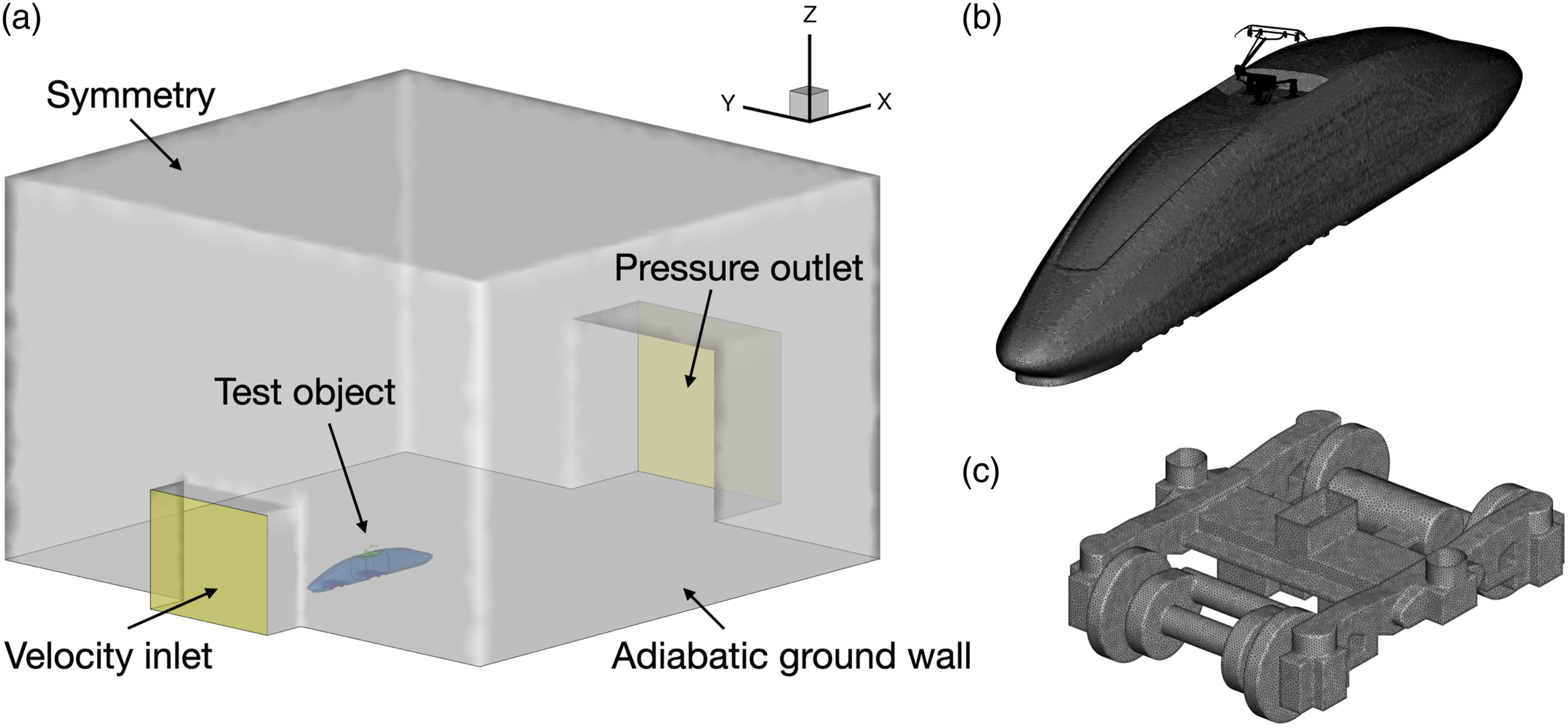

The computational grid is generated using Ansys ICEM. For the volume mesh, tetrahedral cells are generated in the free stream space and 5 layers of prism cells are generated over the solid wall surfaces for capturing boundary layer flow, which results in y+ value of around 30. Local mesh refinement is applied in the region of interest, namely the underbody and pantograph regions. The resulting grid has 13.8 million volume cells and 3.4 million nodes. Figures 7(b) and 7(c) show the surface mesh on the train body and bogie, respectively.

For the numerical simulation of particle motion, snow particles are seeded uniformly upstream of the test object, with initial state in equilibrium with the surrounding air flow. The injected particles have density 200kg/m³ and mean diameter 200μm, which are representative of light small snow particles. Aerodynamic drag is modelled using Morsi and Alexander.³⁶ and gravity is included in the simulation. The second order Crank-Nicolson scheme is used with physical time step of 1e-5s.

The test object surface, namely the prisms, train body, bogie and pantograph, are treated as reflect condition. The wind tunnel walls and inlet and outlet are treated as escape conditions and all other boundaries are set as trap condition. In the current study, the normal and tangential coefficients of restitution for reflect condition are set as 0.01 and 0.1 respectively, to avoid unnecessary elastic behaviour during collision. In addition, particles impacting the wall at an angle smaller than 45°and with a local friction velocity magnitude smaller than 0.21 m/s will be trapped.

For snow accumulation and ice accretion predictions, the quasi-steady approach using local collection efficiency is adopted. For ice accretion, the Myers model³³ is used with Implicit Euler scheme and physical time step of 0.1 s. The spatial density of the particle is set as 10g/m³; this value was obtained from the average of experimental particle measurements. The test object surface temperature is treated as equal to the ambient air temperature.

Validation against simple prism object measurements

In this section, the icing predictions by HADICE is validated against experimental measurements for the simple prism objects.

Figure 8 shows the top view of the simulated snow particle trajectories impinging on the three prism objects. In these plots, the outline of the prisms are highlighted and the particle trajectories are coloured by the instantaneous particle velocity magnitude. Particle deceleration near the frontal surfaces and acceleration around the sides can be observed. The collision spots can be clearly identified at the locations where particle velocity drops to nearly zero. Moreover, a ‘vacuum-like’ zone is identified at the rear of the prisms, which represents the wake region unreachable by any trajectory due to the inertia effect. Based on the simulated trajectories, it is anticipated that mass accumulation occurs mainly on the frontal surfaces.

Figure 8.

Simulated snow particle trajectories impinging on the three prism objects, top view.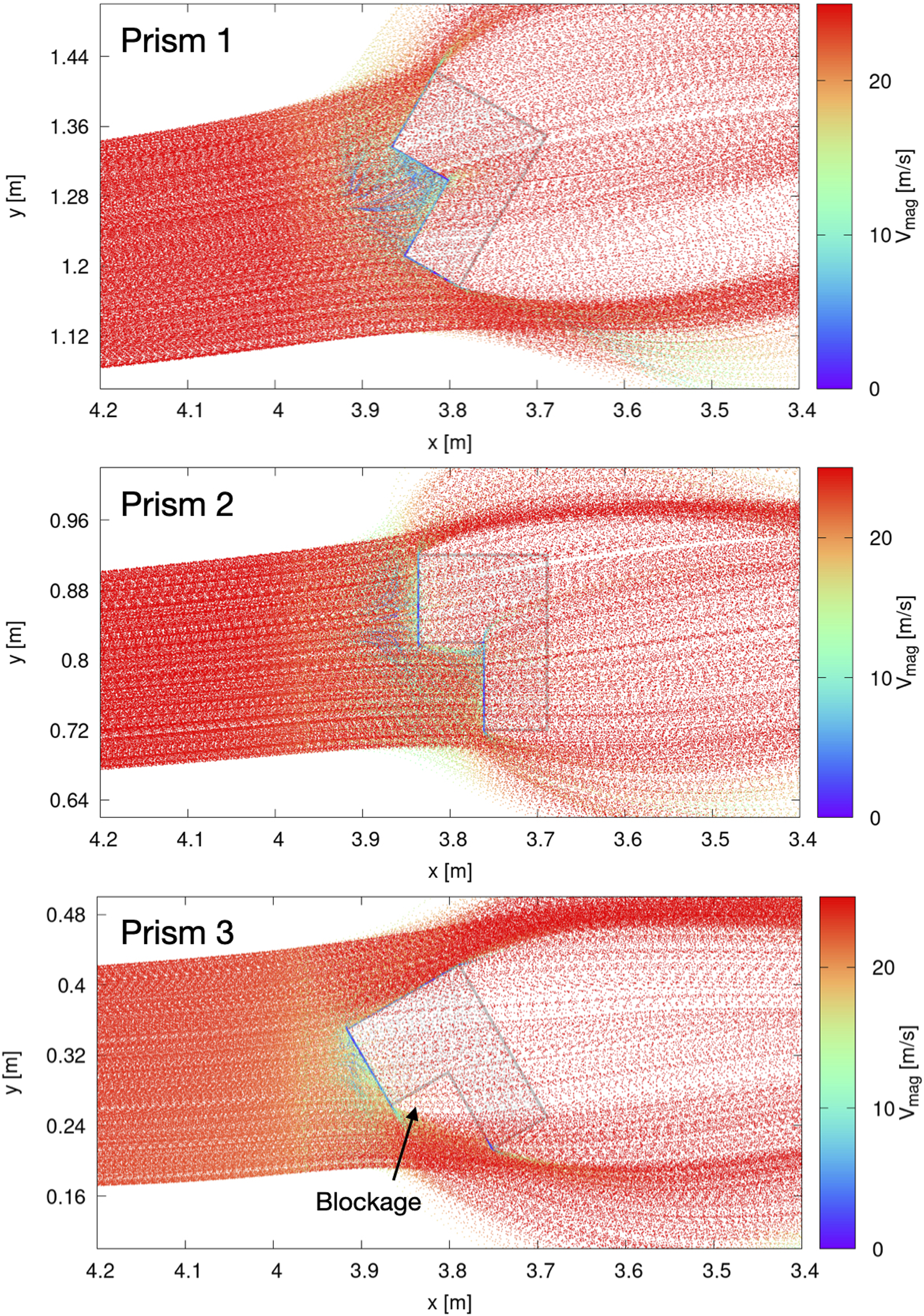

Figure 9 shows the comparison of simulated ice shape with photos taken after the experiment for prisms 1 and 3. The simulation results are overlayed with contour of local collection efficiency. The results are obtained after 5 min of sustained snow injection. In Figure 9(a), it can be seen that ice accretion on Prism 1 occurs on both the front and side surfaces. The overall ice shape is adequately captured by the simulation, however, the ice thickness is slightly under-predicted on the front surfaces and over-predicted on the side surfaces. It is suspected that the discrepancy in spatial deposition might be caused by a slightly different free stream flow angle, as can be seen by the transverse flow angle shown in Figure 8. Possible reason for this discrepancy could be the simplification in wind tunnel inlet geometry in the CFD model. Furthermore, the total mass of accumulated ice on the object is compared between experiment and simulation. The experimental ice mass was measured after the test by removing all the ice from the object surfaces. A total of 1.19 kg was obtained in the experiment compared with 1.05 kg predicted by the simulation. The accumulated mass is adequately simulated with an underestimation of about 12%.

Figure 9.

Comparison of ice shape: (a) Prism 1; (b) Prism 3.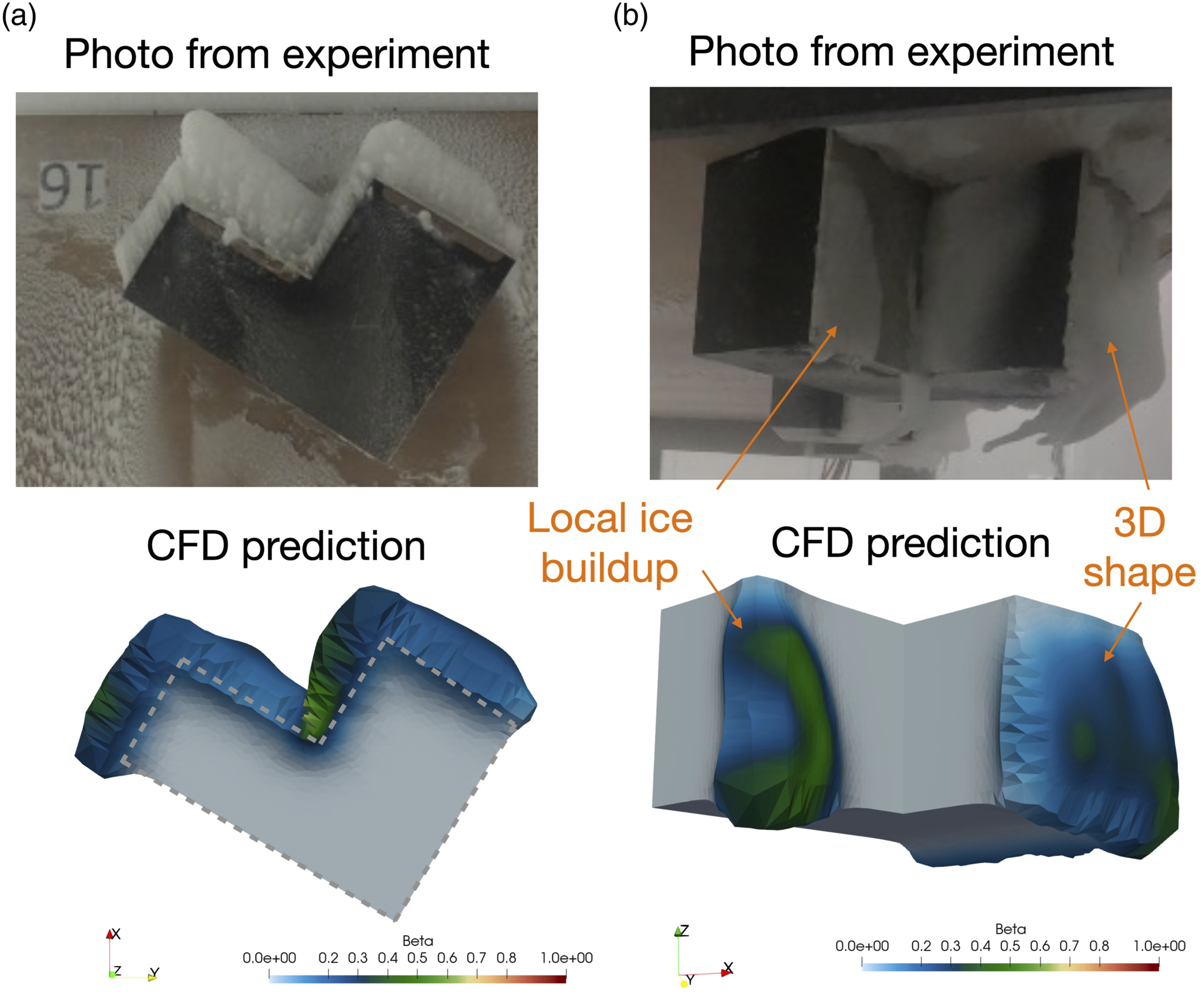

A slightly different icing behaviour is observed in Figure 9(b) for Prism 3. Unlike the other two prisms, both experimental photo and simulation results show that ice accretion only occurs on part of the Prism 3 front surfaces. The cause for this behaviour can be explained using Figure 8, where a particle vacuum zone can be observed in the concave corner due to physical blockage and flow separation. Consequently, most of the particles collide with the leading front surface; a small amount of particles, from the free stream as well as reflected from the leading front surface, collide with the edge of the secondary front surface. The result is the localised ice formation as shown in Figure 9(b). This phenomenon is well captured in the simulation.

Snow accumulation and ice accretion on 1:8 scaled high-speed train model

In the next step, the results for snow accumulation and ice accretion on a high-speed train model are presented. The aim is to demonstrate the capability of the developed simulation framework for real 3D engineering applications. The results presented in this section correspond to 5 min run time with snow particle spatial density 10g/m³ at injection.

Figure 10 shows the snow accumulation on the train body. Photos after the experiment are included for comparison. The simulation results are shown using contour of local collection efficiency on the train body surface. It can be seen that the main accumulation occurs at the front nose of the head car. Snow accumulation on the pantograph can also be observed from the figure. The simulation results are in agreement with the experiment.

Figure 10.

Snow accumulation on the train body surface.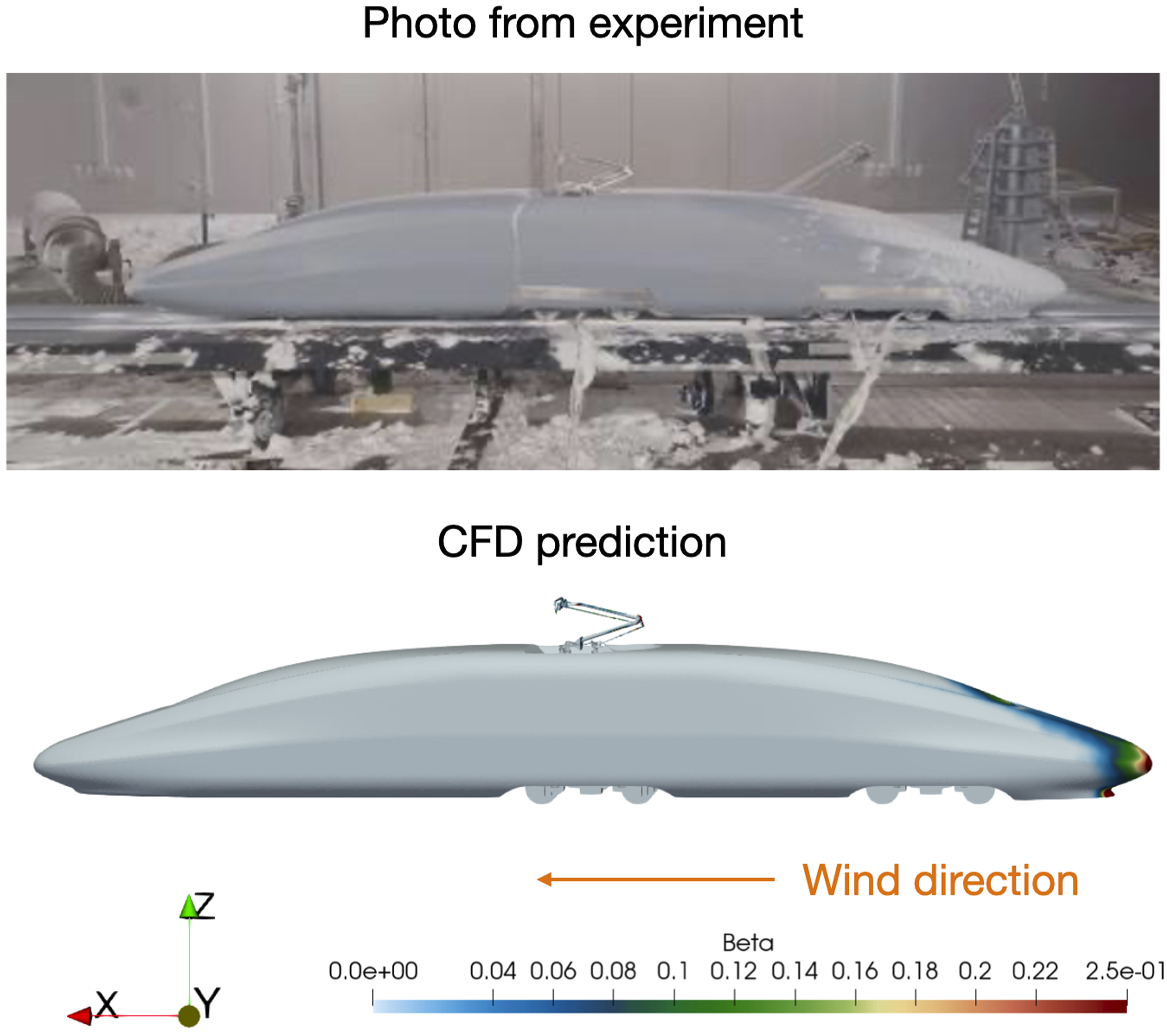

Figure 11 shows the simulation predicted shape change due to accumulation on the pantograph; the simulation results are contoured by the local collection efficiency magnitude. The simulation predicts a maximum thickness of approximately 32 mm on the front surfaces, which is slightly under-predicted compared to the 38 mm recorded in experiment. The locations of highest snow accumulation are well captured by the simulation.

Figure 11.

Snow accumulation on the pantograph.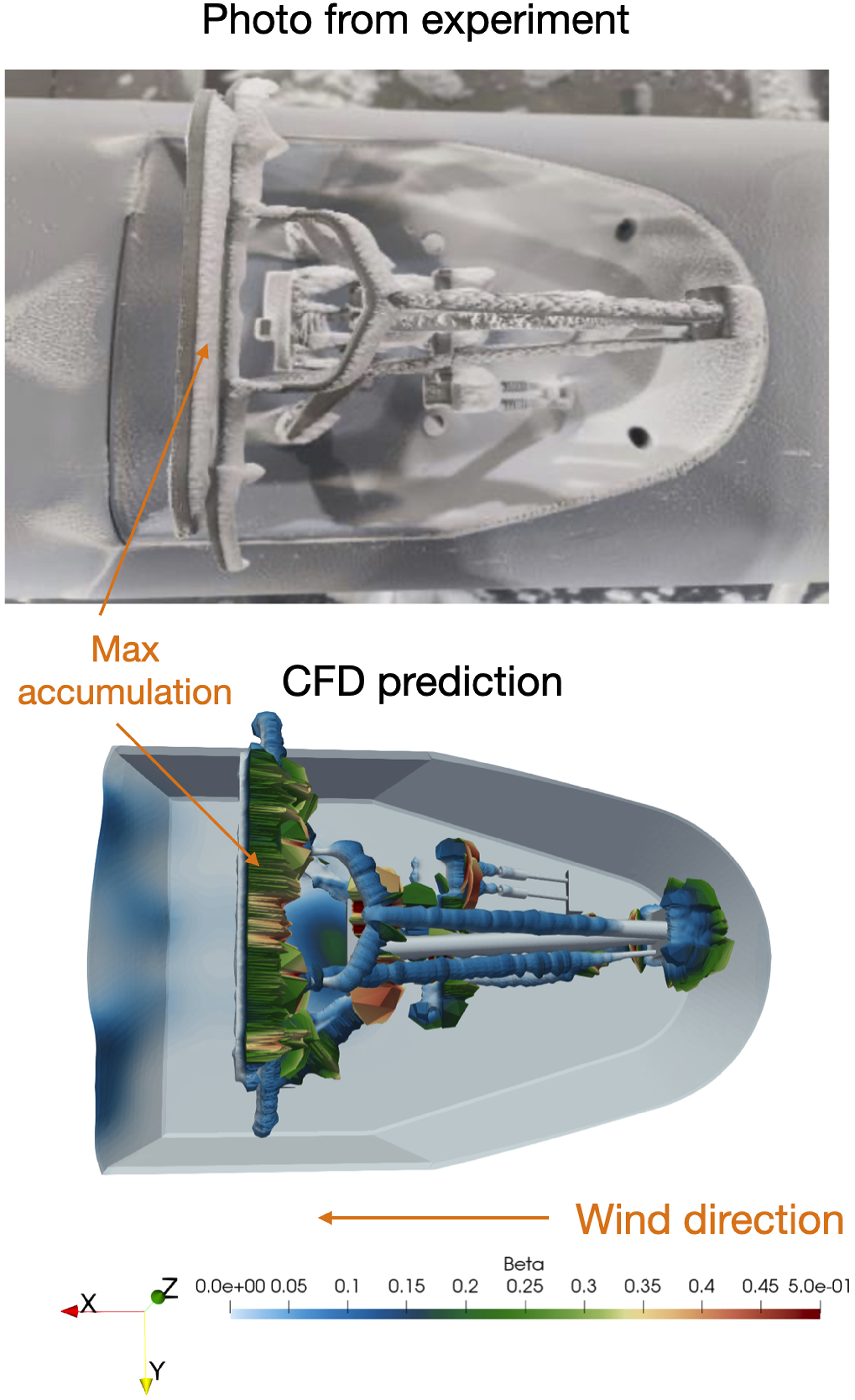

Figure 12 shows the snapshot of calculated snow particle cloud in the mid bogie. Two viewing angles, namely the side view and the bottom view, are shown in this figure. In the figure, each coloured dot represents the instantaneous location of a particle where the colour denotes its velocity magnitude. It can be seen from the figure that substantial amount of particles enter the bogie cavities. The upward motion of particles can be attributed to the aerodynamic effects where flow streamlines from the main flow path migrate into the cavities. Moreover, particle collision with the frontal surfaces of structural components and the top and back surfaces of the shroud wall can be observed, which contribute to the accumulation of snow. The predicted results show qualitative similarities with recent experimental and numerical observations for snow accumulation in train bogies.^2,7

Figure 12.

Snapshot of calculated snow particle cloud in the mid bogie at t = 0.5 s since initial injection: (a) Side view; (b) Bottom view (half of the injected particles are hidden).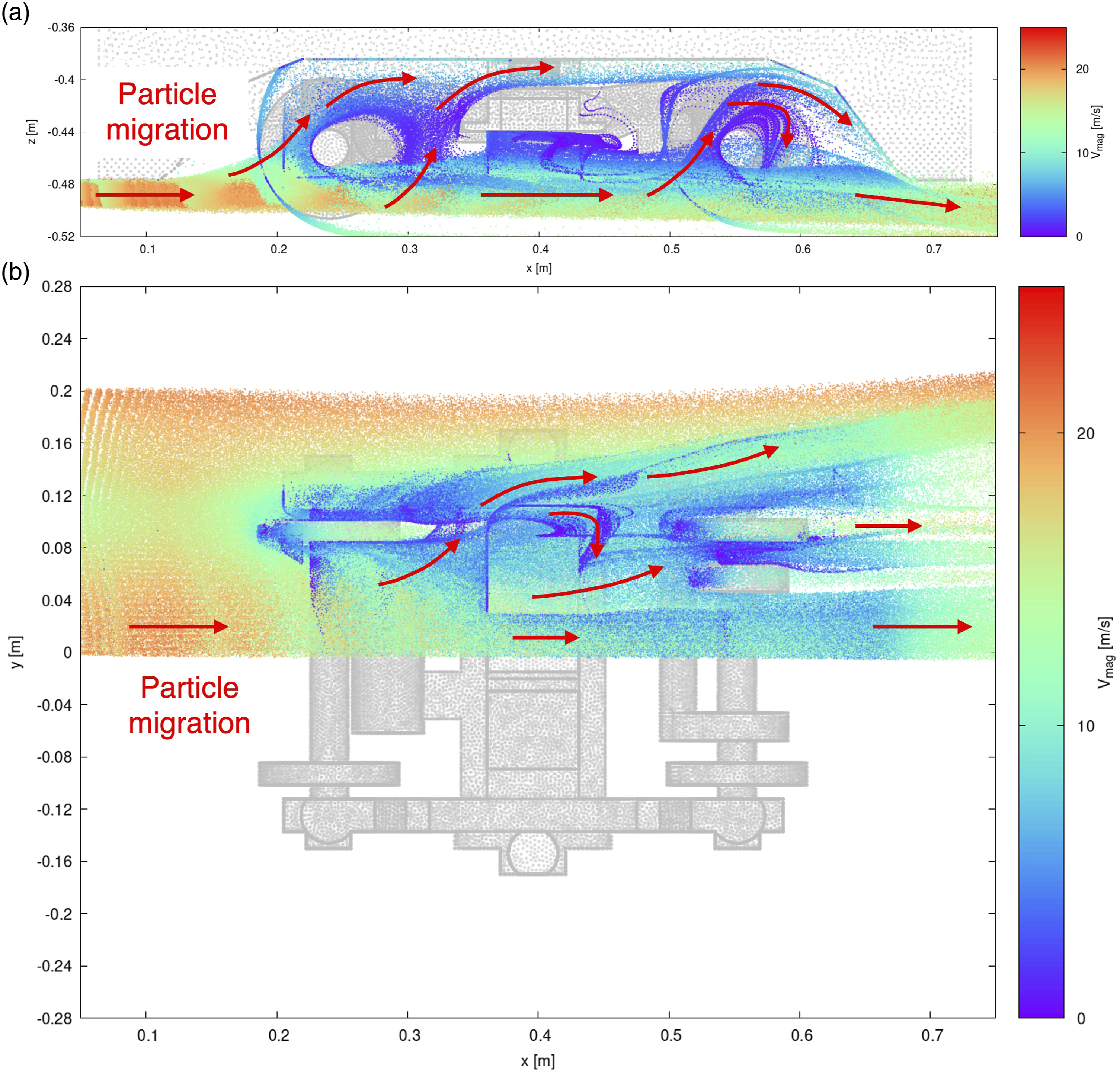

Figure 13 shows the predicted iced geometry for the mid bogie with the surface contour of local collection efficiency. The simulation results shown here correspond to the worst scenario where all the accumulated snow was melted and subsequently froze into ice. In the experiment, heating was provided at only selected surfaces such the gearbox casing and motor box. Physical inspections in the experiment revealed that the heating is sufficient for melting snow, but not large enough so that ice formation on the surface becomes impossible, hence the assumption taken in the simulation. As seen in Figure 12, accumulation can be seen on the front surfaces of structural components. High accumulation spots can be seen at the wheels, gearbox casing and rear wheel shaft. In the experiment, icing was also observed on the heated surface of the rear wheel shaft.

Figure 13.

Iced geometry for the mid bogie. Contour: ice thickness.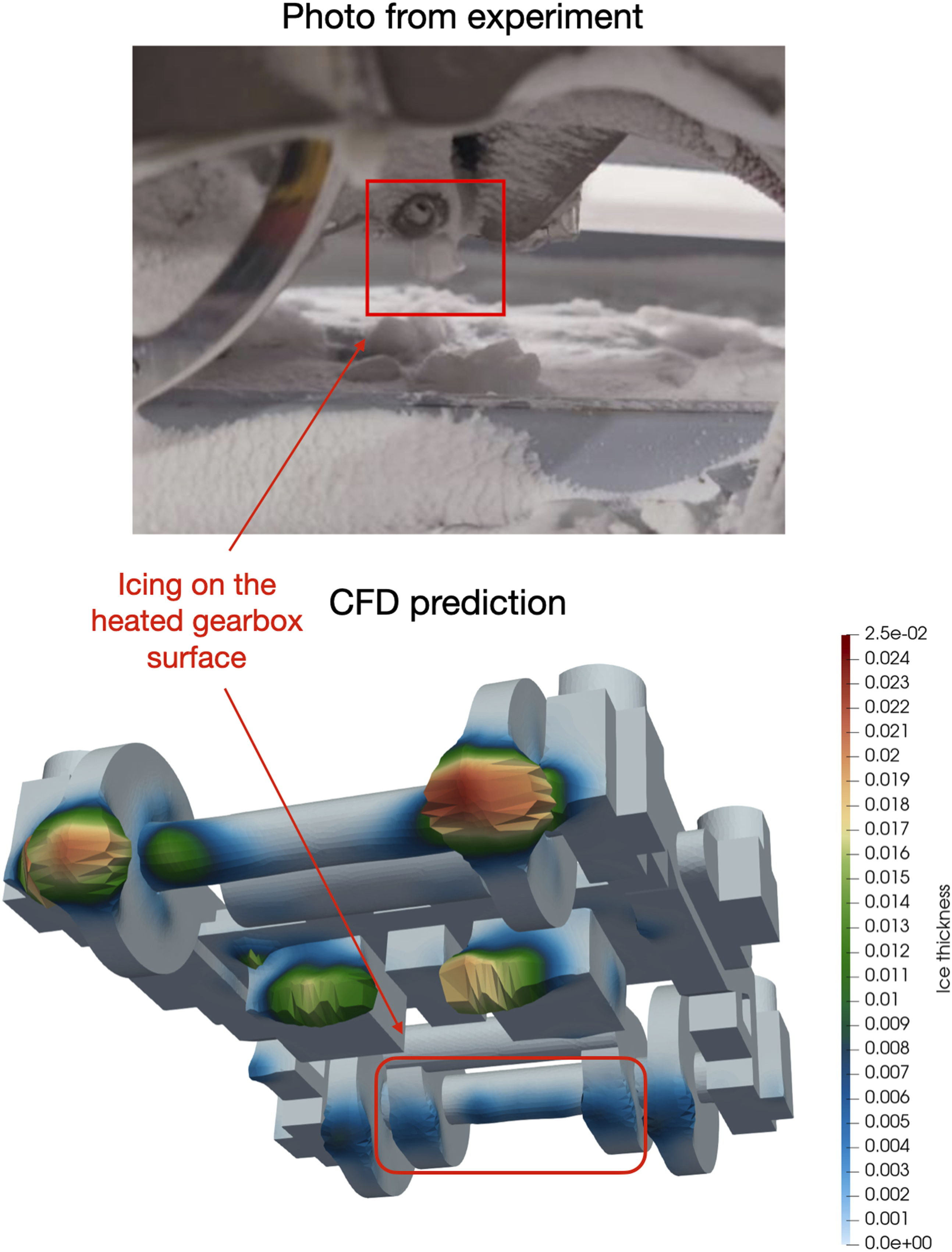

Conclusion and further work

This paper presents the development and validation of a simulation framework HADICE, which adopts a parallel in-house code for simulating three-dimensional particle trajectory and ice accretion in high-speed flows. The air flow is solved using URANS, with optional hybrid RANS/LES capabilities for modelling complex turbulent flows. Particle trajectory tracking is performed using a Eulerian-Lagrangian approach and wall collision is modelled using a hard collision model with reflect condition. Particle accumulation can be obtained either through direct unsteady simulation over a finite time period, or using a quasi-steady approach by evaluating the local collection efficiency. A new iterative method for calculating the local collection efficiency is proposed, which can be used for arbitrary 3D geometry and flow in an accurate and robust manner. Iced geometry is updated through mesh deformation using a RBF interpolation method. Snow accumulation and icing predictions using HADICE were validated against experimental wind tunnel test measurements. A full 3D snow accumulation and ice accretion simulation on a scaled high-speed train model was demonstrated, showing the capability of the presented simulation framework.

In the future, the accuracy and efficiency of the developed code can be further assessed and improved in several aspects. Current model shows consistent under-predictions in the accumulation mass compared with experiment, indicating that the influence of particle trap criteria on the resultant local collection efficiency distribution should be investigated and further re-calibration of coefficient are needed. Another feature that is not captured by the current model is the water run back. For complex convex and concave 3D surface geometries, water run back requires careful modelling so that a realistic flow path is obtained.

Footnotes

Acknowledgements

The authors acknowledge CRRC Qingdao Sifang Co., Ltd For sponsoring this work.

Declaration of conflicting interests

The author(s) declared no potential conflicts of interest with respect to the research, authorship, and/or publication of this article.

Funding

The author(s) received no financial support for the research, authorship, and/or publication of this article.

ORCID iD

Fanzhou Zhao

References

Crowe

Schwarzkopf

Multiphase Flow Handbook. 2 ed. Boca Raton: CRC Press, 2016. DOI: 10.1201/9781315371924

Paradot

Allain

Croué

, et al. Development of a numerical modelling of snow accumulation on a high speed train. Civil-Comp Proc 2014; 104: 1–17. DOI: 10.4203/ccp.104.34

Xie

Zhang

Gao

, et al. Study of snow accumulation on a high-speed train's bogies based on the discrete phase model. J Appl Fluid Mech 2017; 10(6): 1729–1745. DOI: 10.29252/jafm.73.245.27410

Liu

Wang

Zhu

, et al. A numerical study of snow accumulation on the bogies of high-speed trains based on coupling improved delayed detached eddy simulation and discrete phase model. Proc Inst Mech Eng F J Rail Rapid Transit 2019; 233: pp. 715–730. DOI: 10.1177/0954409718805817

Wang

Gao

Liu

, et al. Numerical study of snow accumulation on the bogies of a high-speed train using URANS coupled with discrete phase model. J Wind Eng Ind Aerod 201; 183: pp. 295–314. DOI: 10.1016/j.jweia.2018.11.003

Wang

Zhang

, et al. Impact of rotation of wheels and bogie cavity shapes on snow accumulating on the bogies of high-speed trains. Cold Reg Sci Technol 2019; 159: 58–70. DOI:10.1016/j.coldregions.2018.12.003

Wang

Zhang

, et al. Impact of bogie cavity shapes and operational environment on snow accumulating on the bogies of high-speed trains. J Wind Eng Ind Aerod 2018; 176: 211–224. DOI: 10.1016/j.jweia.2018.03.027

Wang

Gao

Zhang

, et al. Anti-snow performance of snow shields designed for brake calipers of a high-speed train. Proc Inst Mech Eng F J Rail Rapid Transit 2019; 233(2): 121–140. DOI: 10.1177/0954409718783327

Wang

Zhang

Xie

, et al. A study of snow accumulating on the bogie and the effects of deflectors on the de-icing performance in the bogie region of a high-speed train. Cold Reg Sci Technol 2018 148: pp. 121–130. DOI: 10.1016/j.coldregions.2018.01.010

10.

Cai

Lou

Liu

, et al. Numerical investigation of the deposition characteristics of snow on the bogie of a high-speed train. Fluid Dynam Mater Process 2020; 16(1): 41–53. DOI: 10.32604/FDMP.2020.07731

11.

Cai

Lou

, et al. Numerical study of dry snow accretion characteristics on the bogie surfaces of a high-speed train based on the snow deposition model. Int J Real Ther 2022; 10(3): 393–411. DOI: 10.1080/23248378.2021.1918589

12.

Bae

Shon

Kwon

, et al. Numerical investigation of snow accumulation on a high-speed train by snow saltation. Int J Real Ther 2022; 11(0): 465–489. DOI: 10.1080/23248378.2022.2094483

13.

Messinger

Equilibrium temperature of an unheated icing surface as a function of air speed. J Aeronaut Sci 1953; 20: pp. 29–42

14.

Ruff

Berkowitz

. Users manual for the nasa ice accretion prediction code (LEWICE). Technical Report NASA Contractor Report 185129, 1990.

15.

Petrosino

Mingione

Carozza

, et al. Ice accretion model on multi-element airfoil. J Aircraft 2011; 48: pp. 1913–1920. DOI: 10.2514/1.C031346

16.

Aliaga

Aubé

Baruzzi

, et al. FENSAP-ICE-Unsteady: Unified in-flight icing simulation methodology for aircraft, rotorcraft, and jet engines. J Aircraft 2011; 48(1): 119–126. DOI: 10.2514/1.C000327

17.

Gori

Zocca

Garabelli

, et al. PoliMIce: A simulation framework for three-dimensional ice accretion. Appl Math Comput 2015; 267: pp. 96–107. DOI: 10.1016/j.amc.2015.05.081

18.

Bidwell

Potapczuk

. Users manual for the NASA Lewis three-dimensional ice accretion code (LEWICE3D). NASA Lewis Research Center, Cleveland, Ohio: Technical Report NASA Technical Memorandum, 1993.105974

19.

Xie

Chen

, et al. Robust and efficient prediction of the collection efficiency in icing accretion simulation for 3D complex geometries using the Lagrangian approach I: an adaptive interpolation method based on the restricted radial basis functions. Int J Heat Mass Tran 2020; 150: 119290. DOI: 10.1016/j.ijheatmasstransfer.2019.119290 https://linkinghub.elsevier.com/retrieve/pii/S0017931019338487

20.

Wright

Porter

Potapczuk

, et al. An automated refinement process for particle trajectory methods in glennICE. In: AIAA AVIATION 2021 FORUM. VIRTUAL EVENT. Reston, VA, United States. American Institute of Aeronautics and Astronautics, 2021. DOI: 10.2514/6.2021-2631 https://arc.aiaa.org/doi/10.2514/6.2021-2631

21.

The Mpi Forum C . Mpi: a message passing interface In: Supercomputing ’93Proceedings of the 1993 ACM/IEEE conference on Supercomputing. Portland, OR, USA. 19-19 November 1993, pp. 878–883. URL. DOI: 10.1145/169627.169855

22.

Roe

. Approximate riemann solvers, parameter vectors, and difference schemes. J Comput Phys 1981; 43(2): 357–372. DOI: 10.1016/0021-9991(81)90128-5 https://www.sciencedirect.com/science/article/pii/0021999181901285

23.

Jameson

Schmidt

Turkel

. Numerical solution of the Euler equations by finite volume methods using Runge Kutta time stepping schemes. In: 14th Fluid and Plasma Dynamics Conference. Fluid Dynamics and Co-located Conferences. 23 June 1981–25 June 1981. Palo Alto, CA, USA. American Institute of Aeronautics and Astronautics. DOI: 10.2514/6.1981-1259

24.

Spalart

Allmaras

. A one-equation turbulence model for aerodynamic flows. In: 30th Aerospace Sciences Meeting and Exhibit. Reston, Virigina: American Institute of Aeronautics and Astronautics, 1992. DOI: 10.2514/6.1992-439

25.

Pope

. Turbulent flows. Cambridge: Cambridge University Press, 2000. https://www.cambridge.org/core/books/turbulent-flows/69322053C06F73F7EB7124915F9256BD.

26.

Zhao

Vahdati

. Detached eddy simulation: recent development and application to compressor tip leakage flow. J Turbomach 2022; 144(1): 011009. DOI: 10.1115/1.4052019 https://asmedigitalcollection.asme.org/turbomachinery/article/144/1/011009/1115511/Detached-Eddy-Simulation-Recent-Development-and

27.

Zhao

Vahdati

. Evaluation of Spalart-Allmaras turbulence model forms for a transonic axial compressor. In: Proceedingd of Global Power Propulsion Society. Chania, Greece. 7th – 9th September, 2020.

28.

Matsumoto

Saito

. Monte Carlo simulation of horizontal pneumatic conveying based on the rough wall model. J Chem Eng Jpn 1970; 3(2): 223–230. DOI: 10.1252/jcej.3.223 http://www.jstage.jst.go.jp/article/jcej1968/3/2/3_2_223/_article

29.

Sommerfeld

. Modelling of particle-wall collisions in confined gas-particle flows. Int J Multiphas Flow 1992; 18(6): 905–926. DOI: 10.1016/0301-9322(92)90067-Q

30.

Bagnold

. The physics of blown sand and desert dunes. Dordrecht: Springer, 1974.

31.

Nishimura

Hunt

JCR

. Saltation and incipient suspension above a flat particle bed below a turbulent boundary layer. J Fluid Mech 2000; 417: 77–102. DOI: 10.1017/S0022112000001014 https://www.cambridge.org/core/product/identifier/S0022112000001014/type/journal_article

32.

Trenker

Payer

Krenn

, et al. Numerical simulation of snow entrainment with application to train undercarriage design. In: NAFEMS World Congr. 30 Apr 2005. Malta.

33.

Myers

. Extension to the Messinger model for aircraft icing. AIAA J 2001; 39(2): 211–218. DOI: 10.2514/2.1312

34.

Hill

. One-dimensional stefan problems: an introduction. England, UK: Longman Scientific & Technical, 1987. Google-Books-ID: 3LjvAAAAMAAJ.

35.

Kedward

Allen

Rendall

Efficient and exact mesh deformation using multiscale RBF interpolation

J Comput Phys 2017; 345; pp. 732–751. DOI: 10.1016/j.jcp.2017.05.042

36.

Morsi

Alexander

. An investigation of particle trajectories in two-phase flow systems. J Fluid Mech 1972; 55(2): 193–208. DOI: 10.1017/S0022112072001806

A framework for simulating snow accumulation and ice accretion on high-speed trains

Abstract

Keywords

Introduction

Background and motivation

Objectives

Simulation framework and methodology

Overview of framework

Aerodynamic flow solver

Particle trajectory tracking

Calculation of accumulation mass

Ice accretion model

3D mesh deformation

Simulation predictions and comparison with experiment

Experimental test

Computational model

Validation against simple prism object measurements

Snow accumulation and ice accretion on 1:8 scaled high-speed train model

Conclusion and further work

Footnotes

Acknowledgements

Declaration of conflicting interests

Funding

ORCID iD

References