Sage Journals: Discover world-class research

Abstract

A wheel impact load detector is used to assess the condition of a railway wheel by measuring the dynamic forces generated by defects. This system normally measures the impact force at multiple points by exploiting multiple sensors to collect samples from different portions of the wheel circumference. The outputs of the sensors are used to estimate the dynamic force as the main indicator for detecting the presence of the defect. This method fails to identify the defect type and its severity. Recently, a data fusion method has been developed to reconstruct the wheel defect signal from the wheel–rail contact signals measured by multiple wayside sensors. The reconstructed defect signal can be influenced by different parameters such as train velocity, axle load, number of sensors, and wheel diameter. This paper aims to carry out a parametric study to investigate the influence of these parameters. For this purpose, VI-Rail is used to simulate the wheel–rail interaction and provide the required data. Then, the developed fusion method is exploited to reconstruct the defect signal from the simulated data. This study provides a detailed insight into the effects of the influential parameters by investigating the variation of the reconstructed defect signals.

Keywords

Railway wheel defect contact condition monitoring signal reconstruction parametric study

Introduction

Severe wheel defects cause high impact forces that damage the railway vehicle as well as the components of the track. Therefore, early detection of the severe defects is important from a safety point of view to prevent costly failures. In addition, identifying the type and the severity of defects including the minor defects is also important for calculating the track access charge,¹ predicting the degradations, and optimizing the required maintenance plan. Several condition monitoring systems have been developed for detecting the defective wheels, but identifying the defects is still an open issue.²

Wheel impact load detectors (WILD) measure the wheel–rail contact force using the strain³ or vibration⁴ sensors mounted on the rail.⁵ WILD exploit the multiple sensors to collect samples from different portions of the wheel circumference. The defective portion of the wheel causes different forces compared to the other portions. Therefore, by monitoring the variation of the measured force in different sensors, the condition of the wheel can be estimated. The common indicator for estimating the wheel condition is the dynamic force which is calculated by subtracting the average of the forces measured by the multiple sensors from their maximum force. This dynamic force is the extra force generated by the defect. This value provides limited information about the defect and fails to identify its type and severity.

In the prior research,⁶ a data fusion method has been developed to reconstruct the wheel defect signal from the wheel–rail contact signals measured by multiple wayside sensors. This fusion method makes a spatial relation between the samples collected by the sensors and the portion of the wheel contacted with the rail. In this way, the outputs of the sensors are mapped over the circumferential coordinate to reconstruct a pattern that is called wheel defect signal. This signal represents the features of the defect⁷ that can be used for identifying the defect type and the severity.⁸

Besides the wheel defect, the reconstructed defect signal can be influenced by other parameters as well. The fusion process should handle the operational range of every influential parameter. Therefore, this paper aims to evaluate the variation of the reconstructed signals as the outputs of the fusion process by the variation of the influential parameters. The output of the fusion process is influenced by several parameters that can be categorized into two main groups. In the first group, the parameters influence the fusion process, make an imperfect measurement, and corrupt the signals reconstructed. Measurement noise, lack of enough number of sensors, and error in estimating the wheel diameter can be mentioned as the parameters of the first group. In the second group, the operational parameters such as the train velocity and axle load change the signals reconstructed. Variations in these parameters lead to variation in the signals reconstructed even when the defect is kept constant and the fusion process works perfectly.

This paper carries out a parametric study to investigate the effect of the influential parameters. For this, the next section presents a brief overview on the fusion method developed in the previous research.⁶ The input of the fusion process is the data modeled by VI-Rail,⁹ which is a multibody dynamics software. VI-Rail simulates the data that will be provided in practice by the multiple sensors. Then, the generated data are exported to MATLAB as the input of the fusion process. Then, the subsequent section explains the procedure of the data generation using VI-Rail, which is followed by section that defines some indicators to assess the variation of the reconstructed signals. A further section presents and discusses the results of the parametric study. Since several parameters influence the reconstruction process, a set of base value is determined for all the parameters, and in each experiment, only a parameter is changed. Therefore, the exact magnitude of the result obtained in each experiment depends on the determined base value. Finally, the last section draws the main conclusion of the paper.

Data fusion method: An overview

The multiple sensors should be installed in the identical positions to give comparable outputs. The common track structure limits the potential locations for installing the sensors. The sensors can for example be installed on the rail above the sleepers to measure the rail strain or the displacement. The locations of the sensors are known as a distance vector (X) with respect to the location of the first sensor.

A wheel has three main positions with respect to a sensor. First, when the wheel is far from the sensor, in which the sensor has zero output. Second, when the wheel is approaching or leaving the sensor, in which the output of the sensor is increasing or decreasing. Third, when the wheel is on top of the sensor, in which the sensor output is maximum and is called the effective zone. The length of the effective zone depends on the physical properties of the sensor and its position on the rail. This is a narrow area in which a limited number of samples can be selected from that.

When M sensors collect N samples on their effective zones, a dataset from the samples is generated as follows

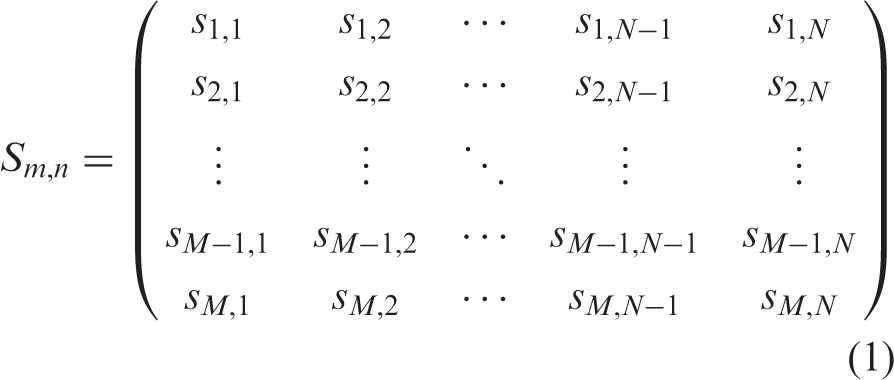
\begin{matrix} S_{m, n} = (\begin{matrix} s_{1, 1} & s_{1, 2} & \dots & s_{1, N - 1} & s_{1, N} \\ s_{2, 1} & s_{2, 2} & \dots & s_{2, N - 1} & s_{2, N} \\ : & : & : & : \\ s_{M - 1, 1} & s_{M - 1, 2} & \dots & s_{M - 1, N - 1} & s_{M - 1, N} \\ s_{M, 1} & s_{M, 2} & \dots & s_{M, N - 1} & s_{M, N} \end{matrix}) \end{matrix}

(1)

This dataset contains the magnitude of the samples collected from the effective zones of the multiple sensors. Each row corresponds to the samples of a sensor. For example, sample s_1,1 is the first sample collected from the wheel on the effective zone by the first sensor. The sample s_2,1 is the first sample collected by the second sensor. The distance between the samples s_1,1 and s_2,1 in the circumferential coordinate is equal the distance between the sensors 1 and 2 that is a known value in vector (X). The length of the wheel circumference is usually provided by maintenance companies and it is a known value. The first column of the dataset that are collected by the multiple sensors can be mapped over the circumferential coordinate using the following equation:

Y_{m, 1} = X_{m} - (L_{w} \times ⌊ \frac{X_{m}}{L_{w}} ⌋)

(2)

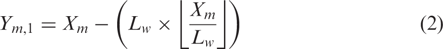
In this equation, X_m is the sensor position vector, L_w is the length of the wheel circumference, $⌊ ⌋$ is the round operator toward the nearest integer less than or equal to the element, and Y_m,1 is the position vector of the first column of the dataset over the circumferential coordinate. The portion of the wheel that is sensed by each sensor is determined using equation (2). In this equation, the sensor location vector is segmented by the length of the wheel circumference. The remainder after division of the sensor location vector (X_m) by the wheel circumference length (L_w) determines the sample position over the circumferential coordinate. Equation (2) uses the first column of dataset 1 and maps them over the circumferential coordinate and is called single sampling method (SSM). For mapping the other samples of the dataset, equation (2) can be extended by using multiple samples and is called multiple sampling method (MSM)

Y_{m, n} = Y_{m, 1} + ((n - 1) \times λ)

(3)

in which

Y_{m, 1}

is the position of the first samples of the sensors, and n is the number of samples in the effective zone. Other samples of the effective zone should be related to the first samples in the space domain. λ is the space interval between the samples that can be defined using the space delay ρ and the samples delay δ as follows

λ = \frac{ρ}{δ}

(4)

The space delay (ρ) is equal to the space distance between the two consecutive sensors which is a known value. Variation in the sleeper distance changes the space delay. When this variation is known, the space delay can be considered as a non-constant parameter using a vector and the fusion method can deal with that. In this research, it has been supposed that the sensors are installed in a specific location with a constant sleeper distance. The sample delay (δ) is estimated using the maximum cross-correlation between the signals measured by the two sensors $z_{1} (i)$ and $z_{2} (i)$ . The cross-correlation function can be calculated as follows¹⁰

R_{z_{1} z_{2}} (γ) = \sum_{i = 1}^{I - γ} z_{1} (i + γ) z_{2} (i), γ = 0, 1, 2, \dots

(5)

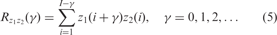
The cross-correlation between the signals $R_{z_{1} z_{2}} (γ)$ involves shifting one of the signals and summing the multiplication of the two signals. Therefore, the cross-correlation is a function of the lag between the signals (γ). The lag γ that maximizes the cross-correlation value presents the sample delay δ.

δ = {argmax}_{γ} R_{z_{1} z_{2}} (γ)

(6)

The wheel velocity can also be estimated using the sampling frequency of the sensor f_t, the space delay (ρ), and the sample delay (δ) as follows

V = \frac{ρ}{δ} \times f_{t}

(7)

Using the magnitude (S_m,n) and the position (Y_m,n) of the samples (M × N samples), the defect signal (ψ_s) is reconstructed:

ψ_{s} = [Y_{m, n}, S_{m, n}]

(8)

To find a more detailed explanation of the fusion method, refer to the prior research.⁶

Generating the simulated data by VI-Rail

VI-Rail is an ad-hoc railway simulation software that has been built upon MSC Adams. VI-Rail as a commercial multibody dynamics software is used to model the dynamic behavior of the rail and the defective wheel to generate the required data. This software models the interaction of the track and the vehicle by considering their subsystems such as sleepers, rail pads, car body, wheelsets, primary and secondary suspensions, dampers, and anti-roll bars.

The first step of generating data by VI-Rail is modeling the defect on the wheel. A precise defect model defines the size, shape, and the position of the defect on the wheel profile and on the wheel circumference. Nielsen and Johansson¹¹ classified the wheel defects and explained the reasons of their development. In this parametric study, a wheel flat with 40 mm length and 0.4 mm depth is modeled. Then, the track and vehicle parameters are defined based on the Manchester Benchmarks¹² for a passenger vehicle. VI-Rail models the wheel–rail interaction for an assembly model that consists of a flexible track and a vehicle. The flexible track is modeled by a straight UIC60 rail in which the mass and inertia properties are concentrated on each rail sleeper. The vehicle has a car body, two bogies, and eight S1002 wheels. The detailed explanation of this model falls outside the scope of this paper.

The fusion method is generic and can be used for different signals including the contact force, the rail to sleeper displacement, and the bending moment. In the prior research⁶ that explains the fusion method, it has been presented that VI-Rail provides a range of outputs such as the contact force, the rail and sleeper acceleration, and the rail and sleeper displacement. The primary desired output is the rail strain signal that is used in practice, but VI-Rail cannot provide that signal. By considering the rail as a transducer, the contact force signal is transformed into the rail response such as strain, acceleration, and displacement. In this research, due to lack of the strain signal, the vertical rail to sleeper displacement is used as the output of the data generation process. Every sleeper is considered as a sensor that measures the rail to sleeper displacement signal. The sleepers have a discrete and periodic configuration like the sensors' configuration.

Result indicators

The fusion process reconstructs a new signal from the signals measured by the multiple sensors. The output of the fusion process is influenced by several parameters such as the train velocity, axle load, defect type, number of sensors, length of the effective zone, and wheel diameter. To evaluate the effect of the influential parameters, a reference signal (ψ_r) is generated to make a comparison with the reconstructed signal (ψ_s). The reference signal is produced when the number of sensors increases to the extent that the samples completely cover the wheel circumference (e.g., 200 sensors). In addition, the reference signal is generated with no measurement noise. For the parametric study detailed in the next section, the number of sensors is less than the number of sensors used for the reference signal and the measurement noise is also considered. In addition, the error of estimating the velocity influences the reconstructed signal. Therefore, a comparison between the reference signal and the reconstructed signal with these errors gives a sense about the results obtained.

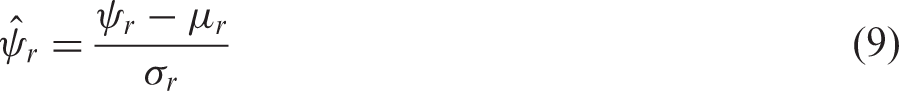
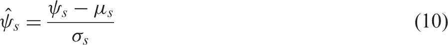
The similarity comparison is carried out using the cross-correlation between the normalized signals. For this purpose, the reference and the reconstructed signals are normalized with respect to their average, and their standard deviation is presented below:

{\overset{\land}{ψ}}_{r} = \frac{ψ_{r} - μ_{r}}{σ_{r}}

(9)

{\overset{\land}{ψ}}_{s} = \frac{ψ_{s} - μ_{s}}{σ_{s}}

(10)

where

{\overset{\land}{ψ}}_{r}

is the normalized reference signal,

{\overset{\land}{ψ}}_{s}

is the normalized reconstructed signal, μ_r and σ_r are the average and the standard deviation of the reference signal, and μ_s and σ_s are the average and the standard deviation of the reconstructed signal.

The samples of the reference signal and the reconstructed signal have non-uniform intervals. Therefore, the signals are interpolated with similar intervals (e.g., 1 mm). ${\overset{\land}{ψ}}_{r}^{*}$ is the interpolated normalized reference signal and ${\overset{\land}{ψ}}_{s}^{*}$ is the interpolated normalized reconstructed signal. These signals have K samples with identical intervals.

The cross-correlation function uses two different signals as the input. The auto-correlation is similar to cross-correlation and based on the Equation (5) while put the same signal as the input. The cross-correlation and the auto-correlation are calculated as follows

R_{{\overset{\land}{ψ}}_{r}^{*}, {\overset{\land}{ψ}}_{s}^{*}} (ζ) = \sum_{k = 1}^{K - ζ} {\overset{\land}{ψ}}_{r}^{*} (k + ζ) {\overset{\land}{ψ}}_{s}^{*} (k), ζ = 0, 1, 2, \dots

(11)

R_{{\overset{\land}{ψ}}_{r}^{*}, {\overset{\land}{ψ}}_{r}^{*}} (ζ) = \sum_{k = 1}^{K - ζ} {\overset{\land}{ψ}}_{r}^{*} (k + ζ) {\overset{\land}{ψ}}_{r}^{*} (k), ζ = 0, 1, 2, \dots

(12)

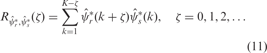
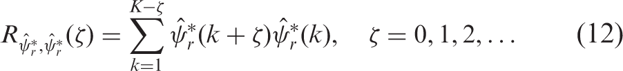
Using equations (11) and (12), the similarity between the reference signal and the reconstructed signal ( ${\tilde{S}}_{ψ_{r}, ψ_{s}}$ ) is calculated as

{\tilde{S}}_{ψ_{r}, ψ_{s}} = \frac{argma x_{ζ} R_{{\overset{\land}{ψ}}_{r}^{*}, {\overset{\land}{ψ}}_{s}^{*}} (ζ)}{argma x_{ζ} R_{{\overset{\land}{ψ}}_{r}^{*}, {\overset{\land}{ψ}}_{r}^{*}} (ζ)}

(13)

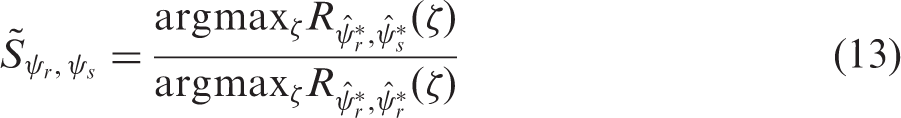
According to this equation, the similarity ranges between 0 and 1, where 1 indicates 100% similarity and 0 indicates no similarity.

To evaluate the performance of the proposed method for estimating the wheel velocity, a comparison is made between the estimated velocity and the actual value used in the data generation step. This comparison presents the absolute errors of the wheel velocity (in m/s) that estimated using the proposed methods.

Furthermore, some parameters have a random nature such as the noises and the position of the defective wheel with respect to the sensors. Therefore, the test is repeated several times and the results are presented as an average of the repetitions with their corresponding standard deviations.

Results of the parametric study and discussion

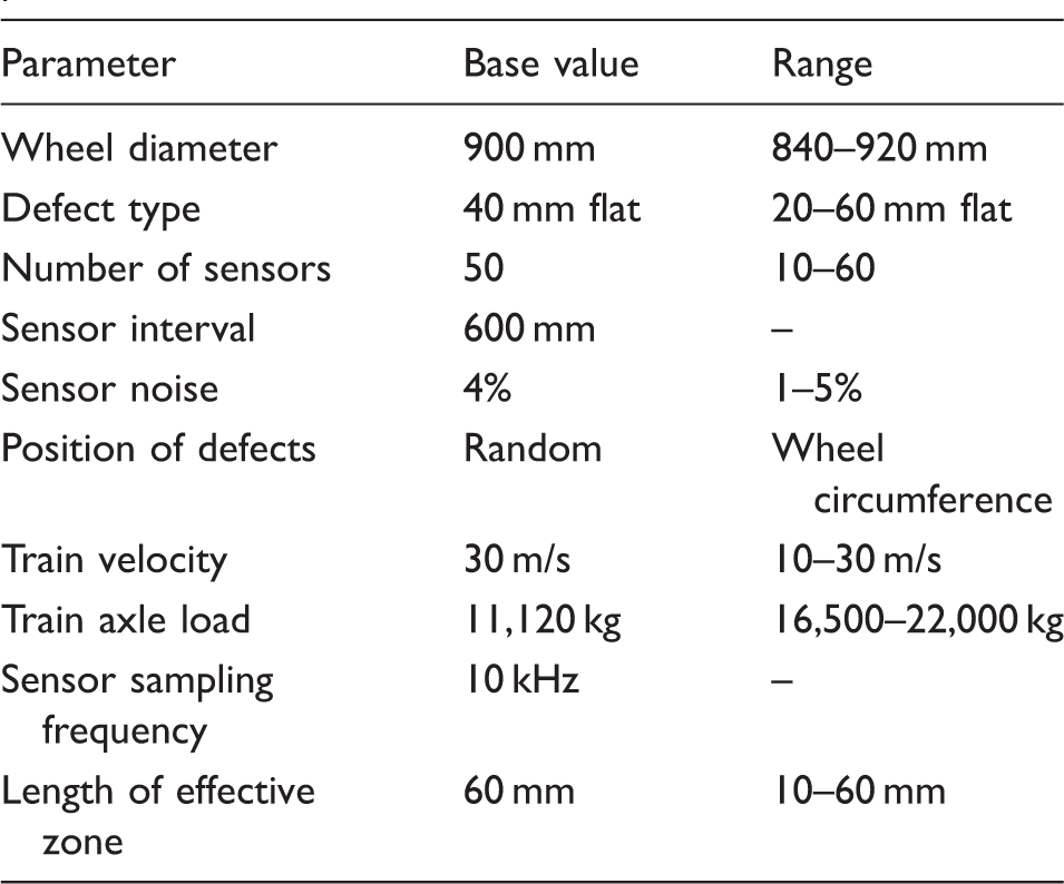
Several parameters influence the output of the fusion process. To evaluate the effect of each parameter, a set of base values is defined. In this section, the results of the fusion process using the base values are presented. In this study, the trends of the results are more important than the exact value. Some parameters are changed over the data generation process and a few others are changed over the fusion process. Table 1 presents the base values with their variation ranges. These parameters are explained and investigated in the following subsections. In every simulation, the base values remain constant except one parameter.

Table 1.

The base value and the variation range of the parameters.

Parameter	Base value	Range
Wheel diameter	900 mm	840–920 mm
Defect type	40 mm flat	20–60 mm flat
Number of sensors	50	10–60
Sensor interval	600 mm	–
Sensor noise	4%	1–5%
Position of defects	Random	Wheel circumference
Train velocity	30 m/s	10–30 m/s
Train axle load	11,120 kg	16,500–22,000 kg
Sensor sampling frequency	10 kHz	–
Length of effective zone	60 mm	10–60 mm

The outputs of the parametric study are the estimated train velocity and the similarity of the signal reconstructed. The MSM uses the train velocity to estimate the distance between the samples collected in the effective zone. To estimate the train velocity, the time delay between the signals measured by the two sensors is used. To achieve this purpose, any pair of sensors can be used. In this research, the consecutive pairs of sensors (e.g., sensor 1 and sensor 2) are used. The train velocity is the average of the estimated velocities by different pairs. For example, for a test with 50 sensors, the average of the velocity estimated by 49 pairs of sensors gives the output. Therefore, the result provides a reasonable estimate of the train velocity. The error of the velocity estimation for the base value using the noise free signal is 0.000639 m/s and its corresponding standard deviation is 0.000312 m/s. By adding the noise to the signal, the error of the velocity estimation increases to 0.0179 m/s and its standard deviation to 0.0119 m/s. Using these velocities, and based on equation (4), the space distances between the samples of each sensor (λ) will be 3.0001 and 3.0018 mm, respectively, for the noise free and the noisy measurements, which are satisfactory values for the data fusion process.

Table 2 presents the results of the similarity evaluation. For the noise free measurement, the MSM improves the similarity from around 50% to 99%. The MSM improves the similarity by using more samples to reconstruct the signal. The measurement noise has a significant effect on the results. Therefore, exploiting the sensors with high signal-to-noise ratio (SNR) is vital. The following subsections assess the influential parameters on the reconstruction process and present the variations of the results to the variation of the parameters.

Table 2.

The comparison between the similarity of the SSM and MSM for the base values.

Indicator	Similarity (%)	Standard deviation (%)
Noise free
SSM	49.95	5.33
MSM	98.58	1.47
Noisy
SSM	28.78	7.14
MSM	52.92	10.52

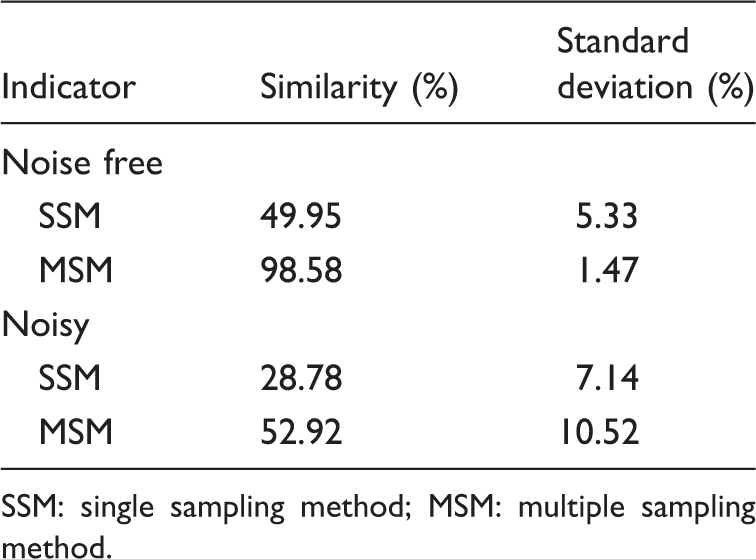
SSM: single sampling method; MSM: multiple sampling method.

Measurement noise

The fusion method is generic and can be used for different signals including the contact force, the rail to sleeper displacement, and the bending moment. In the prior research⁶ that explains the fusion method, it has been reported that VI-Rail provides a limited range of outputs such as the contact force, the rail and sleeper acceleration, and the rail and sleeper displacement. The primary desired output is the rail strain that is used in practice, but VI-Rail cannot provide the rail strain signal. By considering the rail as a transducer, the contact force signal is transformed into the rail response such as strain, acceleration, and displacement. In this research, due to lack of the strain signal, the vertical rail to sleeper displacement is used as the output of the data generation process. Every sleeper is considered as a sensor that measures the rail to sleeper displacement signal. The sleepers have a discrete and periodic configuration similar to the sensors' configuration.

VI-Rail generates pure data while the real measurements will be noisy. Therefore, evaluating the effect of the measurement noise on the fusion process is vital. To make a realistic assumption about the SNR, the results of a field test that used fiber Bragg grating (FBG) strain sensors are considered.¹³ That measurement shows at least 120 $μ ɛ$ variation in the strain signal due to the wheel passage, while the noise was less than 5 $μ ɛ$ (4%). In this study, the minimum variation in the rail to sleeper displacement signal is 200 µm. Therefore, the maximum magnitude of the noise should be less than 8 µm (4%). To simulate the noisy measurement, a set of White Gaussian Noises is added to all signals generated by VI-Rail. The average of the noises is 0 and three times of the standard deviation (3σ) is 8 µm. Figure 1 presents the rail to sleeper displacement signals before and after adding noise.

Figure 1.

The rail to sleeper displacement signals: (a) noise free and (b) noisy.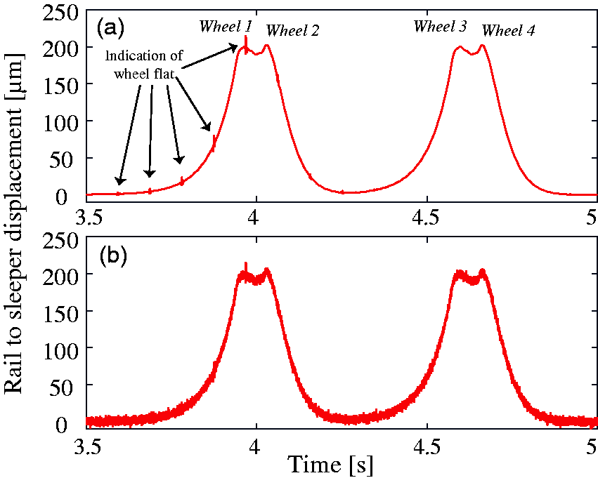

The measurement noise has several negative effects on the fusion process. First, the measurement noise makes an error on the sample delay (δ) between the measured signals. This error leads to errors in the sample distance (λ) and in the wheel positioning. Another negative effect of the measurement noise is the variation of the sensor output.

Figure 2 presents the absolute error of the estimated velocities for different measurement noises. As we expected, increasing the measurement noise increases the magnitude and the standard deviation of the error of the velocity estimated. Figure 2 also presents the errors of the estimated velocities after filtering the signals. The low-pass filter cuts out the high frequency components from the input signals measured. As a result, the error of the velocity estimation process, the error of the sample distance (λ), and the error of the wheel positioning (sampling error) can be reduced, while the negative effects on the variation of the sensor output remain.

Figure 2.

The results of the velocity estimation process for different measurement noises and for the filtered signals.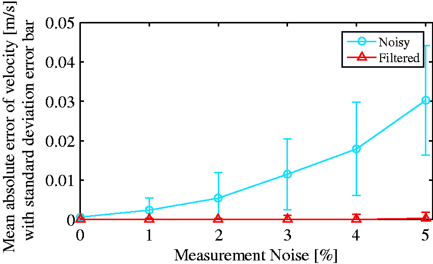

Figure 3 shows the results of the similarity assessment for different measurement noises. The MSM improves the similarity of the reconstructed signals when the noise is not high. By increasing the measurement noise, the similarity significantly decreases. The measurement noise changes the magnitude of the sensor output. The fusion method considers the position and the magnitude of different samples to generate a pattern. Therefore, the small measurement noise can influence the signals reconstructed. According to Figure 3, the 5% noise decreased the similarity of the reconstructed signals from around 100% to less than 50%. As a result, using sensors with high SNR) is critical to produce informative signals.

Figure 3.

The results of the similarity assessment for different measurement noises. SSM: single sampling method; MSM: multiple sampling method.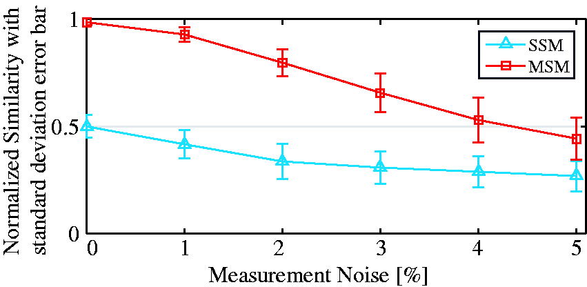

In the further research, the reconstructed signals will be fed into a classification model generated using the pattern recognition methods to be classified into different classes. Therefore, the minimum acceptable similarity level depends on the classification model that will be studied later.

Number of sensors

The fusion method exploits the data collected by the multiple sensors. The signal reconstruction with a few number of samples leads to a signal distortion. Intuitively, more sensors collect more samples and give better results. The sensors should be mounted on the identical positions that is challenging for a measurement with high number of sensors. Therefore, providing similar results with lower number of sensors is essential. A commercial interrogator with four measurement channels can interrogate around 160–320 FBG sensors, fulfilling practical requirements by providing high number of sensors and high SNR.¹⁴

According to equation (7), the velocity is a function of the sample delay (δ) that is estimated using the cross-correlation between the signals measured by different sensors (see equations (5) and (6)). The measured signals have been modeled as the combination of the signal generated by the wheel movement, the signal generated by the wheel defect, and the uncorrelated noises. For the noise free measured signal, the defect signal influences the output of the cross-correlation function. As explained earlier, the velocity is calculated by averaging the estimated velocities by multiple pairs of sensors. The low-pass filter that was used in the prior subsection can cancel out the negative effect of the defect signal and the measurement noise. Figure 4 presents the results of the velocity estimation process for different number of sensors for the filtered signals. Increasing the number of sensors influences the average of the errors and decreases their standard deviations.

Figure 4.

The results of the velocity estimation process using the filtered signals for different number of sensors.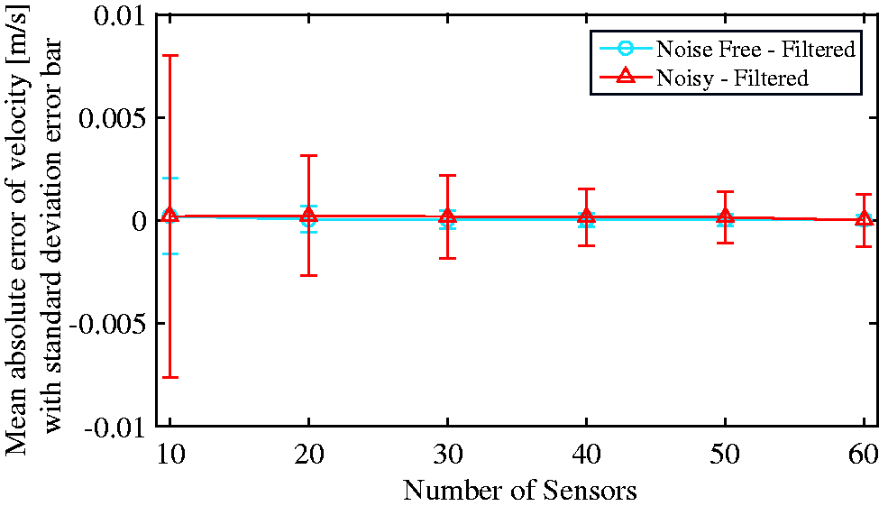

Figure 5 compares the results of the similarity between the SSM and MSM while the number of sensors increases. The MSM collects multiple samples to fill the gaps between the data collected by the SSM and improves the similarity. As a result, increasing the number of sensors increases the similarity.

Figure 5.

The results of the similarity assessment for different number of sensors. SSM: single sampling method; MSM: multiple sampling method.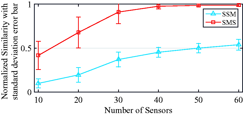

Length of the effective zone

The data generated by VI-Rail is the rail to sleeper displacement signal. The effective zone for this signal is around 60 mm that is constant in all simulations. Therefore, to evaluate the effect of the effective zone variations, different lengths from the effective zone are used. Figure 6 compares the similarity of the signals reconstructed using the SSM and MSM with different lengths of the effective zone. Increasing the length increases the similarity. Therefore, using a sensor with longer effective zone can reduce the number of sensors required. To design an effective measurement system, the length of the effective zone and the number of sensors should be considered in a way that the samples cover entire wheel circumference.

Figure 6.

The similarity comparison between the signals reconstructed by the SSM and MSM for different lengths of the effective zone. SSM: single sampling method; MSM: multiple sampling method.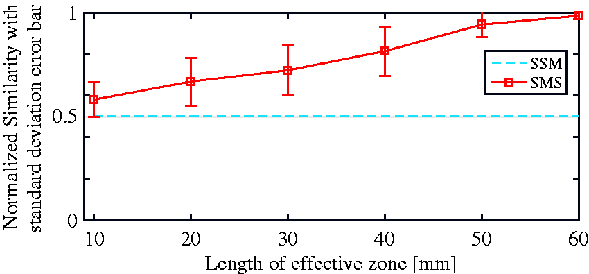

In a simulation study or in a laboratory test, in which the experiment is completely under control, exploiting high number of sensors is viable, while in practice, using a detector with 320 sensors is challenging. The number of sensors and the length of the effective zone should be considered in a way that the collected samples cover the entire wheel. Using the combination of two shear sensors to provide wider effective zone helps a lot to reduce the number of sensors required.

Wheel diameter

For a certain sensor configuration, the wheel diameter is the factor that determines the frequency of the measurement from the wheel circumference in the space domain. The measurement frequency for the range of wheel diameters (840–920 mm¹⁵) will be 4.39–4.81 measurements per cycle for the 600-mm sensor interval. This variation determines the distribution of the samples over the circumferential coordinate. Figure 7 presents an example of the distribution of the samples over the circumferential coordinate for different wheel diameters. In this example, the simulated samples collected by 150 sensors using the SSM with 600-mm sensor interval. The numbers on top of the circles present the wheel diameter and the numbers inside the circles indicate the maximum distance between the samples mapped over the circumferential coordinate.

Figure 7.

The distribution of the samples over circumferential coordinate for different diameters. The numbers on top of the circles present the wheel diameter and the numbers inside the circles indicate the maximum distance between the samples.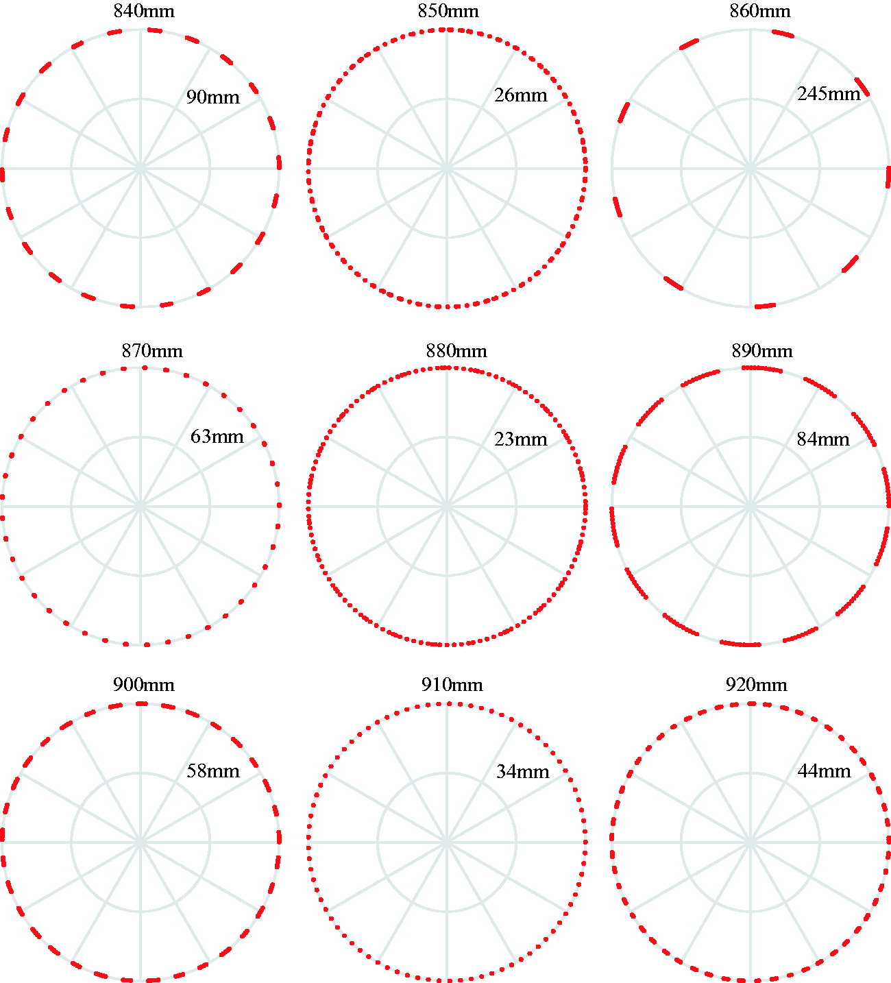

Several parameters influence the distribution of the samples such as the sensor interval, wheel diameter, length of the effective zone, number of sensors, and the train velocity. These parameters with the exception of the number of sensors are the out-of-control parameters. The samples should cover the entire wheel circumference to reconstruct the signal properly. According to Figure 7, the wheel diameter changes the distribution and the frequency of the samples. The monitoring system should be able to cover the whole range of the wheel diameter. Therefore, the required number of sensors should be determined based on the range of the wheel diameter. Figure 8(a) presents the defect signal reconstructed over circumferential coordinate for a wheel with 40 mm flat and 30 m/s velocity. The defect signal after the reconstruction is interpolated to have 1000 samples per meter with a uniform interval in the space domain. Figure 8(b) presents the defect signal in the frequency domain using the fast Fourier transform. This figure shows that the frequency of the signal is limited to the frequencies lower than 100 Hz. It means that the Nyquist frequency in the space domain is 200 samples per meter (twice the highest frequency contained in the signal). Therefore, the defect signal can be reconstructed without any distortion, if the maximum distance between the consecutive samples is smaller than 5 mm.

Figure 8.

(a) The signal reconstructed over circumferential coordinate by 59 sensors using the MSM for a wheel with 850 mm diameter, 40 mm flat, and 30 m/s velocity and (b) the frequency spectrum of the signal.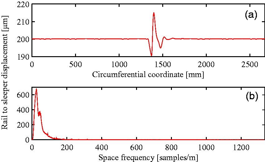

The results of the similarity assessment are presented in Figure 9. The comparison between the results obtained from Figures 7 and 9 shows that the wheel with large distance between the samples has low similarity and the wheel with small distance between the samples has high similarity. The MSM by filling the gaps between the samples using more samples improves the similarity.

Figure 9.

The results of the similarity for different wheel diameters. SSM: single sampling method; MSM: multiple sampling method.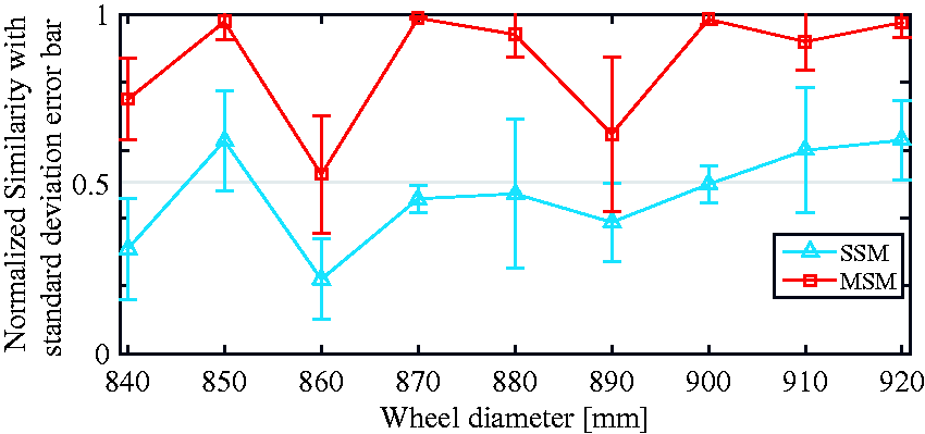

Train velocity

Train velocity influences the fusion process by changing the contact force and the space sampling frequency. A defective wheel exerts different dynamic forces when moves with different velocities, which influences the rail responses and the results obtained. Figure 10 depicts the contact force ratio for different train velocities. The contact force ratio shows the deviation of the dynamic contact force generated by the defect from the static force generated by the wheel load. In this research, the contact force signal is calculated by VI-Rail, and the ratio of the maximum and the average of the signal gives the contact force ratio.

Figure 10.

The contact force ratio for different train velocities.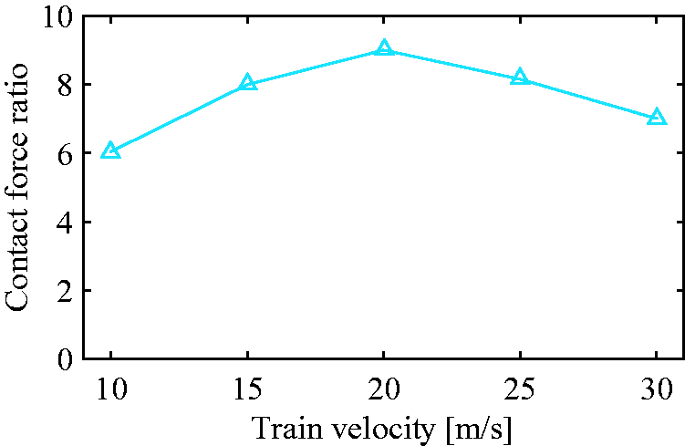

The sampling frequency of the sensors in the space domain depends on the train velocity. Increasing the train velocity decreases the sampling frequency of the space domain. Therefore, increasing the train velocity increases the space intervals between the samples (λ) while the samples are collected in the constant time interval. The contact force ratio has the same effect on the SSM and MSM, while the train velocity directly influences the MSM by changing the sampling frequency in the space domain. Lower train velocity gives higher sampling frequency in the space domain in which the MSM gives better performance.

The velocity estimation process uses the cross-correlation to find the delay between the signals measured by the two sensors. The train velocity changes the contact force ratio that influences the cross-correlation and consequently the estimated velocity. On the other hand, by increasing the train velocity, the space sampling frequency decreases. As a result, by increasing the train velocity, the error of the estimated velocity will be increased. For the noise free measurement, the contact force ratio has the dominant role, while for the noisy measurement, the signals are covered by the noise and the space sampling frequency plays the major role. Figure 11 presents the error of the velocity estimated for different train velocities. Higher sampling frequency of the sensors in the time domain can compensate the effect of high velocity on the sampling frequency of the space domain. Figure 12 presents the results of the velocity estimation process using the filtered signals for different velocities when the input is the noise free signal and the noisy signal. The filter can exclude the effect of contact force and noises but the effect of decreasing the space sampling frequency still remained. Therefore, increasing the velocity increases the error of the estimated velocities.

Figure 11.

The results of the velocity estimation for different train velocities.

Figure 12.

The results of the velocity estimation process using the filtered signals for different train velocities.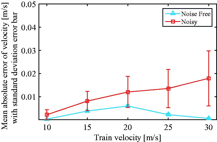

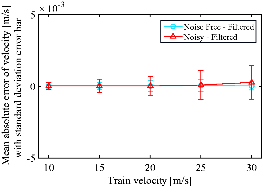
Figure 13 compares the similarity of the signals reconstructed by the SSM and MSM for different train velocities. Clearly, the MSM is performing better than the SSM especially for the lower velocities. As mentioned earlier, lower train velocity leads to higher space sampling frequency. Therefore, with constant length of the effective zone, higher samples are collected. For example, a sensor with 10 kHz sampling frequency and 60 mm effective zone collects 60 samples with 1 mm distance from a train with 10 m/s velocity, while it collects 20 samples with 3 mm distance from a train with 30 m/s velocity.

Figure 13.

The similarity comparison between the signals reconstructed by the SSM and MSM for different train velocities. SSM: single sampling method; MSM: multiple sampling method.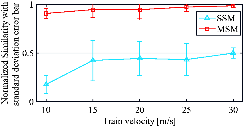

Defect type

The variation in the defect type and size changes the contact force and the contact force ratio and consequently changes the rail response. This subsection studies the wheel flat as the most severe defect. Figure 14 presents the contact force ratio for flats with different lengths. Increasing the defect size increases the contact force ratio.

Figure 14.

The contact force ratio for different defect types.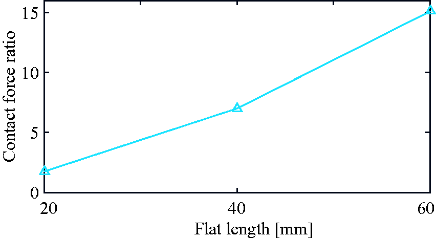

Figure 15 presents the results of the similarity assessment using the SSM and the MSM for different defect sizes. Increasing the defect size increases the similarity. The MSM has better results than the SSM. For minor defects, the measurement noise covers the defect signal and decreases the similarity. Therefore, using the sensors with high SNR is essential for reconstructing the defect signal for the minor defects.

Figure 15.

The results of the similarity assessment for different defect types. SSM: single sampling method; MSM: multiple sampling method.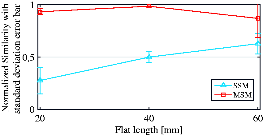

Figure 16 presents the results of the velocity estimation process for different defect sizes. The measurement noise increases the errors of the estimated velocities. In addition, the defect size changes the contact force ratio. Therefore, for the severe defects, the defect size is the dominant factor and causes the error. As mentioned earlier, the input signals can be filtered to suppress the negative effects of the noise and the defect signal on the velocity estimation process.

Figure 16.

The results of the velocity estimation for different defect types.

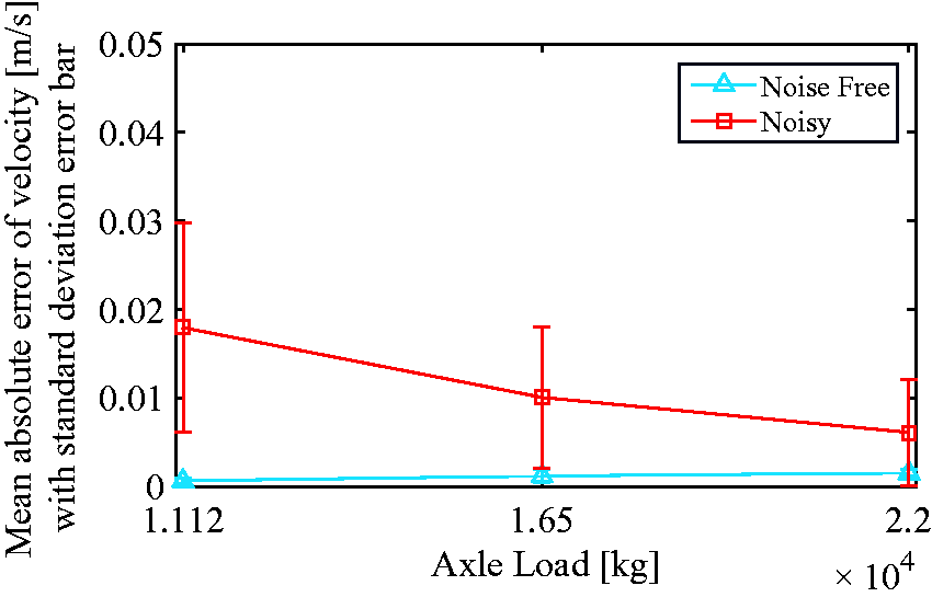
Axle load

The mass of the car body (32,000 kg), the bogie (2615 kg) and the wheelset (1813 kg) are based on the Manchester benchmarks.¹² Accordingly, the total mass is 44,482 kg and the axle load is 11,120 kg. To assess the effect of the axle load variation on the fusion process, two other axle loads, 16,500 kg and 22,000 kg, are used. The contact force ratio is almost constant for 11,120, 16,500, and 22,000 kg axle loads, i.e., 7, 7.3 and 6.9, respectively. Therefore, different axle loads generate similar defect signals. As a result, axle load variations do not influence the fusion process directly.

The results of the similarity assessment and the velocity estimation process for different axle loads are presented in Figures 17 and 18. As we expected, the variations of the axle load have slightly changed the results. By increasing the axle load, the contact force ratio remains almost constant but the static load (average load) is increased. Therefore, the ratio of the noise to the main signal decreases. As a result, increasing the axle load decreases the effect of the noise and improves the results. This consequence is visible in the estimated velocities for the noisy signals.

Figure 17.

The results of the similarity assessment for different axle loads. SSM: single sampling method; MSM: multiple sampling method.

Figure 18.

The results of the velocity estimation for different axle loads.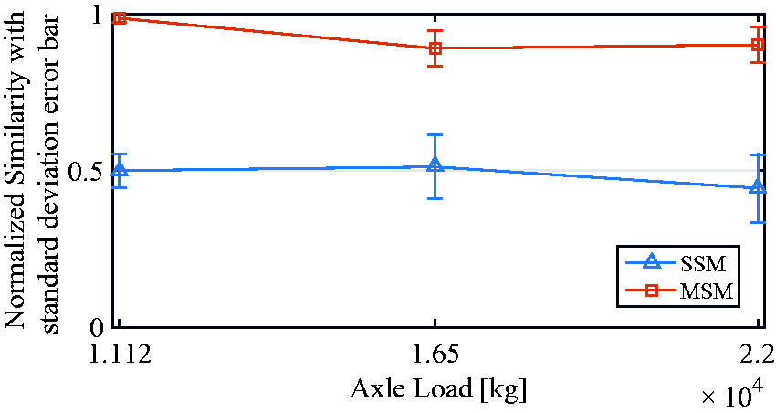

Conclusion

The wayside wheel monitoring systems such as the WILD normally measure the rail responses by the multiple sensors to estimate the condition of the passing wheels. The developed fusion method reconstructs a new signal from the data collected by the multiple sensors. The output of the fusion process is influenced by several parameters. Some of them affect the input of the fusion process and some of them change the performance of the process. This paper carried out a detailed parametric study to investigate the influential factors. A summary of the main conclusions is presented here.

The SSM picks only a single sample per sensor while the MSM exploits all the collected samples (of the effective zone) to fill the gaps between the samples used by the SSM. The results showed the effectiveness of the MSM. When the contact force ratio is not relatively large, the rail response variation due to the wheel defect is comparable with the measurement noise magnitude. Therefore, the measurement noise covers the defect signal and decreases the similarity of the reconstructed signal to around 50% from 97%. It shows that the fusion method can give better performance when the SNR is high. As a result, for detecting the minor defects, using the sensors with high SNR are essential. A low pass filter can only be used in the velocity estimation process to cancel out the negative effect of the defect signal and the measurement noise.

Several parameters influence the distribution of the samples over the circumferential coordinate such as the sensor interval, wheel diameter, train velocity, length of the effective zone, and number of sensors. In general, increasing the number of sensors improves the results of the fusion process. Therefore, a trade-off is required between the cost of the interrogator supporting high number of sensors, and the accuracy and reliability of the fusion results. In addition, using the sensors with longer effective zone reduces the number of sensors required. Furthermore, the sampling frequency of the sensors limits the maximum velocity of the wheel that can be monitored.

The reconstructed defect signal can be influenced by material properties and in general is a function of the track and vehicle dynamics. It has been supposed that these properties are constant over the measurements. By considering all these parameters, a condition monitoring system can be designed to perfectly reconstruct the wheel defect signal that can be used for the identification of the defect.

Footnotes

Declaration of Conflicting Interests

The author(s) declared no potential conflicts of interest with respect to the research, authorship, and/or publication of this article.

Funding

The author(s) disclosed receipt of the following financial support for the research, authorship, and/or publication of this article: This work was partly supported by the Ministry of Science, Research and Technology of the Islamic Republic of Iran (MSRT).

References

European Commission, Commission implementing regulation (EU) 2015/909. Off J Eur Union 2015; 2015: 17–22.

Alemi

Corman

Lodewijks

. Condition monitoring approaches for the detection of railway wheel defects. Proc IMechE, Part F: J Rail and Rapid Transit 2017; 231: 961–981.

Stratman

Liu

Mahadevan

. Structural health monitoring of railroad wheels using wheel impact load detectors. J Failure Anal Prevent 2007; 7: 218–225.

Belotti

Crenna

Michelini

, et al. Wheel-flat diagnostic tool via wavelet transform. Mech Syst Sign Process 2006; 20: 1953–1966.

Partington

. Wheel impact load monitoring. Proc ICE – Transport 1993; 100: 243–245.

Alemi

Corman

Pang

, et al. Reconstruction of an informative railway wheel defect signal from wheel–rail contact signals measured by multiple wayside sensors. Proc IMechE, Part F: J Rail and Rapid Transit. 2019; 233: 49–62.

Alemi A, Pang Y and Lodewijks G. In-service detection of defective railway wheels with periodic out-of-roundness. In: Z Li and A Nunez (eds) 11th international conference on contact mechanics and wear of rail/wheel systems (CM2018), Delft, The Netherlands, 24–27 September 2018, pp.25–30.

Alemi A, Pang Y, Corman F, et al. Railway wheel defect identification using the signals reconstructed from impact load data. In 11th International workshop on structural health monitoring, Stanford, CA, pp.1511–1518. California: DEStech Publications, Inc.

VI-Grade Engineering Software & Services. VI-Rail 16.0 documentation. Technical report, VI-grade GmbH, Marburg, Germany, 2014.

10.

Knapp

Carter

. The generalized correlation method for estimation of time delay. IEEE Trans Acoust Speech Signal Process 1976; 24: 320–327.

11.

Nielsen

JCO

Johansson

. Out-of-round railway wheels – a literature survey. Proc IMechE, Part F: J Rail and Rapid Transit 2000; 214: 79–91.

12.

Iwnicki

. Manchester benchmarks for rail vehicle simulation. Vehicle Syst Dynam 1998; 30: 295–313.

13.

Tam

Lee

, et al. Utilization of fiber optic Bragg Grating sensing systems for health monitoring in railway applications. Struct Health Monitor 2007; 2: 1824–1831.

14.

Wei

C-L

Lai

C-C

Liu

S-Y

, et al. A fiber Bragg grating sensor system for train axle counting. IEEE Sens J 2010; 10: 1905–1912.

15.

UIC Leaflet. UIC 510-2 OR, trailing stock: wheel and wheel sets conditions concerning the use of wheels of various diameters. Technical report, UIC, Paris, France, May 2004.

Evaluation of the influential parameters contributing to the reconstruction of railway wheel defect signals