Investigating railway track asset management using a Markov analysis

Abstract

A railway track asset management strategy must ensure that the condition of the track stays at an acceptable level, ensuring passenger comfort and safety. The determination of an efficient and effective strategy is a complex problem that requires consideration of the interrelated processes of deterioration, inspection, maintenance and renewal. Railway traffic causes the track’s geometry to deteriorate through time. When the track’s geometry has been assessed and seen to have deteriorated, maintenance is scheduled to restore the track’s geometry using a tamping machine. Tamping involves lifting the track to the required position before inserting vibrating tines into the ballast either side of the sleepers and using them to pack the ballast below. This process causes damage to the ballast, causing a relative acceleration in future track geometry deterioration and decreasing the time between subsequent maintenance interventions.

This paper describes a Markov model that can be used to investigate the asset management strategy applied to a railway track section. The model predicts the way that the track section’s condition changes with time for a given asset management strategy, which is defined through the specification of a number of model parameters. The model is applied to a track section with a specified maintenance strategy and is used to investigate the track’s performance for that strategy. Parameters corresponding to asset management decisions that relate to inspection, maintenance and renewal are then changed in order to illustrate the effects of the decisions on the track’s life cycle. The Markov model provides a simple yet powerful means of investigating the effects of an asset management strategy on a railway track section.

Introduction

A railway track’s geometry deteriorates with use due to settlement of the ballast and/or other supporting layers such as the formation. Minor deterioration can affect the ride quality experienced by passengers whereas more extreme deterioration has the potential to cause far more serious issues such as a derailment. It is therefore of vital importance that all track around the network is maintained to an acceptable level of quality. The track’s geometry is restored by adjusting the ballast below the sleepers; this maintenance can be performed either manually or by using tamping or stoneblowing machines. In the UK a track’s geometry is assessed at regular intervals of time using a measurement train, it is used to determine the quality of the track over 220 yard (1/8 mile) sections. The information obtained by the measurement train is used to inform decisions as to where and when maintenance is required. When the geometry falls below an acceptable level, maintenance is scheduled to restore the geometry to an acceptable condition. If the condition worsens before maintenance is performed then, in the interests of safety, speed restrictions are imposed until the maintenance can take place. In the worst case, line closures may be required, although these are rare. These speed restrictions and line closures affect the operations of the trains timetabled to use the track and can result in heavy penalties for the network operator based on the number of delays and cancellations that result.

The goal of a railway asset management strategy is to determine how best to apply maintenance to keep the track’s quality at an acceptable level, in terms of both passenger comfort and safety, in an efficient, cost-effective manner. As in many industrial systems, maintenance is a significant factor in the financial performance of the railway. Track asset management has been investigated using a number of stochastic models. These aim to combine the deterioration and maintenance processes to predict the change in track condition over time.

Models have been developed that represent the track’s condition as an artificial track quality index (TQI), this is a linear combination of a number of measures of the track’s geometry.^1-3 A TQI with a range of 100, based on unevenness, twist, alignment and gauge measurements, was used in a five-state Markov model to investigate track performance. ⁴ A 50-state Markov model was used to investigate track twist and optimise inspection frequency and applied to straight, curved or transition track sections. ⁵ Podofillini et al. ⁶ and Kumar et al. ⁷ applied stochastic RAMS approaches to rail failure modelling. A multi-objective optimisation approach was applied in Podofillini et al. ⁶ to determine an optimal inspection frequency.

Quiroga and Schnieder^8,9 used deterioration and maintenance data from the French railway operator, SNCF, in a statistical model of the track’s condition to investigate the application of different maintenance strategies. A cost-effective strategy was identified using Monte Carlo simulation.

A Petri net (PN) model has been developed in order to investigate the performance of individual track sections ¹⁰ using deterioration time distributions derived from UK rail network data. ¹¹ The PN model was further developed to allow a number of track sections to be modelled, meaning that all or part of the entire rail network can be investigated. ¹² The PN model forms a framework for Monte Carlo simulations to be performed to investigate the effects of an asset management strategy. ¹³

Since the PN models are well-suited to the analysis of a wide variety of maintenance and asset management strategies, they can become large and complex. A Markov model of a track section was developed that is simpler in structure than the PN model and allows the asset management of a single track section to be investigated at a basic level. ¹⁴ In this paper, a base-case model of the asset management of a track section is developed. The model is then used to investigate the variation of the asset management strategy by varying parameters relating to inspection, maintenance and renewal.

Track asset management

Railway track asset management involves the scheduling of inspection and maintenance to respectively monitor and counteract the effects of track deterioration.

Inspection

Traffic loading causes a gradual deterioration in the track’s quality through time as the forces from passing trains cause settlement, wear and break-up of the ballast that is used to support the sleepers and rail. Specially-instrumented recording vehicles are used at regular intervals to obtain data that is processed to give measures of the geometry over sections of the railway track. In the UK these sections have a length of 1/8 mile. The following track geometry measures are produced.

Vertical geometry (top) - rail height standard deviation (SD) (left, right and mean), subtracted from a 35 m (short-wave) or 70 m (long-wave) running average.

Lateral geometry (alignment) - rail alignment, averaged over the left and right rail, expressed as short- and long-wave SDs.

Gauge - rail spacing compared to the standard gauge.

Cyclic top - a measure of resonant dip frequencies (which may cause a train to ‘bump’ along the track, possibly leading to a derailment).

Twist - a measure of cant variation over 3 and 5 m.

All of these measures are compared against a specific set of acceptable values ¹⁵ and if these values are exceeded maintenance must be scheduled in order to rectify the associated geometry fault in the track. The short-wave measurement of the vertical geometry is generally the most significant measurement when determining a track’s condition and requirement for maintenance. The specified acceptable limits for the measurements of a track section’s vertical geometry depend on the permissible speed for that track section. The greater the track speed, the lower the acceptable limits. ¹⁵

Track maintenance

If the measured vertical geometry of a track section deteriorates to such an extent that the maximum permitted acceptable limit is exceeded then action is needed. Maintenance must be performed to restore the track’s condition such that the geometry is acceptable once more or speed restrictions must be imposed to a level where the measured SD of the vertical geometry is less than the maximum acceptable limit at that speed. Maintenance involves packing ballast beneath the sleepers in order to correct the alignment of the rails and hence improve the track’s quality. Manual intervention can be performed, although this is clearly only suitable for short lengths of track in urgent situations. Generally, the track’s geometry is improved using either tamping machines or stoneblowers.

Tamping machines work by measuring the track’s geometry, calculating the required adjustment, lifting the track precisely to the desired position and inserting vibrating tamping tines either side of the sleeper. The vibrating tines squeeze the existing ballast below the sleeper, packing it in such a way that once the track is released the required alignment is retained. Tamping can therefore be used to improve the track’s quality; however, every time tamping is performed the process of inserting the vibrating tines and squeezing the ballast causes some break-up of its constituent stones. This break-up affects how well the stones interlock (and hold the track in position following maintenance) and also how well water can drain through the ballast. Hence, the process of tamping causes the ballast’s condition to deteriorate and negatively affects its future performance.

Stoneblowing machines work in a similar way to tampers, in that they measure the track’s condition and lift it precisely to the required level. However, rather than forcibly redistributing the existing ballast beneath the sleepers, stoneblowers work by pneumatically injecting smaller stones into the void beneath the sleepers in order to hold the track in position. Stoneblowing does not cause ballast break-up like tamping; however, once stoneblowing has been performed on a track section tamping can no longer be performed in the future. This is because tamping would cause the small stones injected by the stoneblower to move down through the ballast and have a detrimental impact on its performance.

Track deterioration

Figure 1 shows a typical plot of the data recorded by a measurement train, indicating the variation of the short-wave measurement of vertical alignment for a 1/8 mile track section through time. The vertical lines superimposed on the plot indicate the times of track section renewal and maintenance interventions extracted from maintenance records. Using such records, it is possible to analyse track deterioration throughout different phases of the track section’s lifetime, with the phases relating to the periods between successive intervention activities and the rate of deterioration changing according to the number and type of interventions that have been carried out previously. The methods used to analyse the data are presented in full in Audley and Andrews. ¹¹ A two-parameter Weibull distribution was used to describe, for different life phases, the distribution of times to deteriorate to any specified level of SD for a track section. The distributions are dependent on the traffic and the types of sleeper and rail in the track section. The Weibull parameters, β (the shape factor) and η (the scale factor or characteristic life), are given as functions of the short-wave SD of the vertical alignment, σ.

Figure 1.

A plot of the variation of the short-wave SD of vertical alignment for a track section and recorded renewal and maintenance interventions.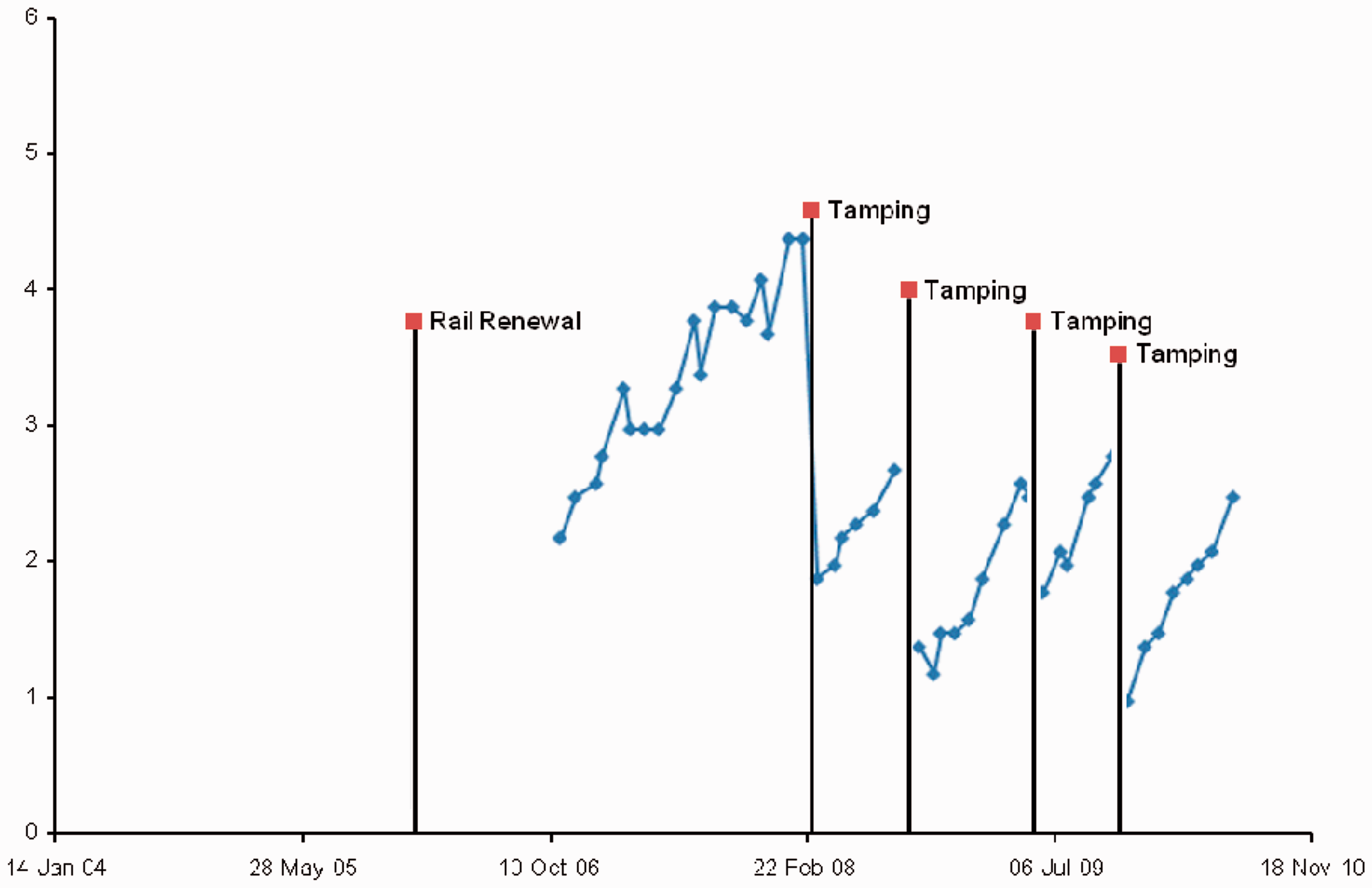

Model of a track section

A Markov model of the asset management of a track section was presented in Prescott and Andrews. ¹⁴ The model considers the effects of maintenance (tamping only) and inspection strategies on the quality of the track section throughout its lifetime from renewal to renewal. The transitions in the model relate to track quality deterioration (as measured by the short-wave SD of the vertical alignment), inspection and maintenance. In building the model, it has been assumed that after seven tamps the ballast has degraded to such an extent that its performance does not deteriorate following further maintenance.

Track quality classification

The states in the model relate to a classification of the track section’s quality as indicated by its short-wave SD of vertical alignment, σ. The following classifications are made:

0 ≤ σ < σ_crit track in good condition (good);

σ_crit ≤ σ < σ_spd maintenance requested (crit);

σ_spd ≤ σ < σ_cls speed restriction required (spd);

σ_cls ≤ σ line closure required (cls).

Here σ_crit is defined as a critical value of the SD of the vertical alignment, which, once discovered to have been exceeded for a track section, triggers a request for maintenance to be performed on that section in order to improve its quality. As the track deteriorates further the SD will reach σ_spd, which corresponds to the maximum permitted acceptable limit for the SD, meaning that speed restrictions must be imposed. If the track then deteriorates further to have an SD of σ_cls then it is assumed that a line closure will be required on that track section.

Markov model’s structure

A section of the Markov model for the analysis of the asset management of a track section is shown in Figure 2. This part of the model relates to the deterioration and inspection of the track section during a single phase of its lifetime, following renewal. It is assumed that the track section lies in one of the four SD bands described at the beginning of the section ‘Track section model’. The track starts in the good condition (good), then the SD deteriorates to such an extent that a critical value is reached at which point maintenance will be requested (crit). Further deterioration leads to a requirement for speed restrictions (spd) or line closures (cls) to be imposed.

Figure 2.

State transition diagram for a Markov model of the deterioration and inspection during a single phase of the track section’s lifetime (following renewal).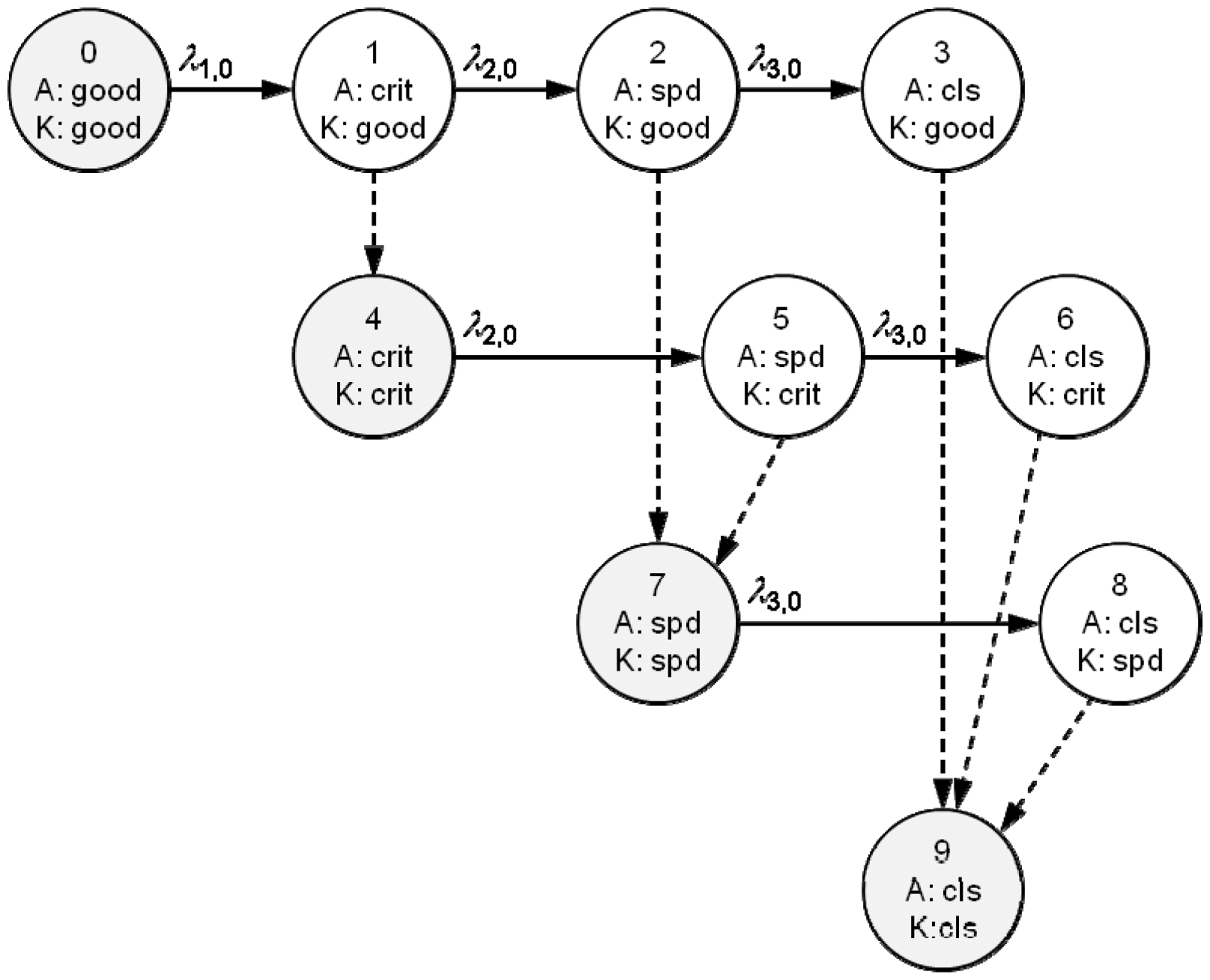

Deterioration and inspection

Ten distinct model states are defined for each phase of the track section’s lifetime. These are identified by considering the actual (A) and the known (K) condition of the track section. The known condition of the track section will only match the actual condition either when the track is in a good condition (in which case both the actual and the known condition are good, as in state 0 in Figure 2) or following an inspection (dashed edges in Figure 2) that reveals that the track has deteriorated to some extent since the last inspection (states 4, 7 and 9). Therefore, in the state transition diagram shown in Figure 2, the shaded states 0, 4, 7 and 9 correspond to the track’s condition being revealed and the remaining states correspond to the track’s condition being unrevealed. For example, for state 1, the actual state of the track is such that the SD of the vertical alignment has reached the critical level at which maintenance is requested (A : crit) but at the last inspection the track quality was observed to be good (K : good).

The deterioration transitions shown in Figure 2 have associated rates λ_{i, j} , where i relates to the level of deterioration of the track section (and j relates to the maintenance history (number of tamps performed in the track section since the renewal).

Maintenance

The entire track section model contains eight sets of 10 states of the form shown in Figure 2, with each set of 10 states representing a single phase of the track section’s lifetime. Separate states are needed for each phase because the condition of the ballast degrades following maintenance and hence the track section’s quality will deteriorate at a different rate following each successive tamp. The 80 model states are numbered from 0 to 79 using the formula 10j + k, where j is the number of tamps that have been performed on the track section (if j > 7 then j = 7 because of the assumption that after seven tamps the performance of the ballast does not degrade any more following further maintenance) and k is a value corresponding to the track conditions described for the states shown in Figure 2. The deterioration and inspection transitions in each set of 10 states for each life phase mirror those presented in Figure 2. The difference comes in the deterioration rates λ_{i, j} , which vary for each of the phases according to the maintenance history, as represented by j.

It is assumed that when maintenance is performed the track quality is returned to a good condition. However, since the ballast degrades the condition will not be as good as new (AGAN). Figure 3 shows a part of the model containing the maintenance transitions corresponding to the first and second tamps of the track section. States 0 to 9 represent the condition of the track section following renewal and states 10 to 19 represent the condition of the track section following the first tamp. This first tamp is represented by the maintenance transitions that lead from states 4 to 9 to state 10, i.e. from states where the track is known to at least be in a condition that requires maintenance to be requested (states 4 to 9) to the state where the track is in a good condition following one tamp (state 10). Corresponding transitions representing the second tamp lead from states 14 to 19 to state 20 (not shown).

Figure 3.

Deterioration and inspection following renewal and a single tamp and the maintenance transitions related to these life phases.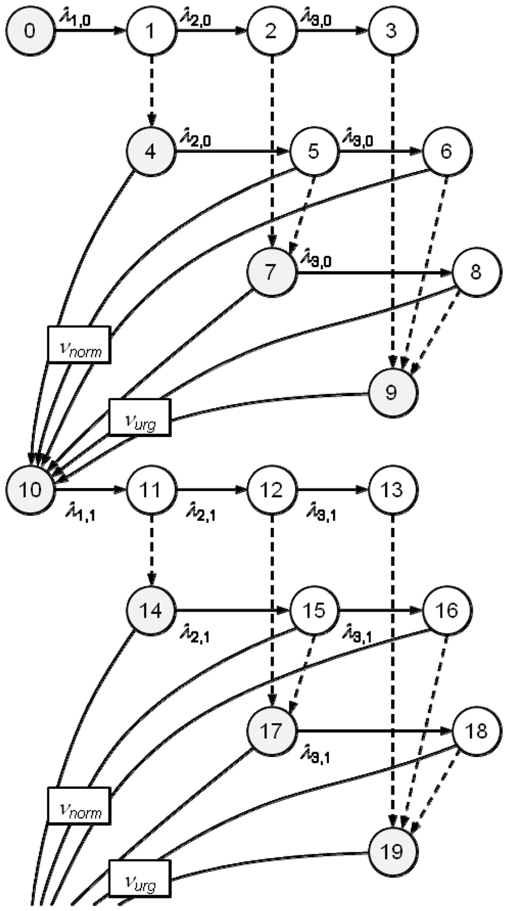

The maintenance transitions each have associated rates ν_norm, corresponding to maintenance of a normal priority that is requested once the SD is known to have exceeded σ_crit, or ν_urg, corresponding to maintenance of an urgent priority that is required when either speed restrictions or line closures must be imposed. Therefore, states 4, 5 and 6 have maintenance transitions that lead to state 10, each with rate ν_norm and states 7, 8 and 9 have maintenance transitions that also lead to state 10, each with rate ν_urg. In general, for number of tamps j < 7, transitions will lead from places numbered 10j + 4, 10j + 5 and 10j + 6 to state 10(j + 1) with rate ν_norm and from places numbered 10j + 7, 10j + 8 and 10j + 9 to state 10(j + 1) with rate ν_urg. Transitions from states 74, 75 and 76 will lead to state 70 with rate ν_norm and from states 77, 78 and 79 will lead to state 70 with rate ν_urg.

Model solution

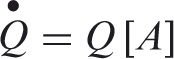
A Markov model containing n states leads to a system of n differential equations of the form:

$Q^{•}=Q[A]$

(1)

where

$Q=[Q_1(t),Q_2(t),\dots ,Q_n(t)]$

(2)

and Q_i(t) is the probability of being in state i at time t. [A] is the n × n transition rate matrix whose elements are defined as:

$A_{\mathrm{ij}}=\{\text{transitionratefromstate}i\text{tostate}\hspace{1em}j\text{if}i\ne j-\sum _{\genfrac{}{}{0ex}{}{k=1}{k\ne i}}^n{A}_{\mathrm{ik}}\text{if}i=j$

(3)

The developed Markov model for the track section therefore leads to a system of 80 differential equations; these can be solved to determine the probability of being in each of the 80 model states. Bespoke C++ software was used to construct and analyse the model. The system of equations was solved numerically using a fourth-order Runge–Kutta algorithm. Inspections were handled during the integration procedure by shifting the appropriate state probabilities at the times in the integration corresponding to the inspection interval of the measurement train.

Model inputs

There are a number of asset management strategies that can be applied that affect the maintenance, inspection and renewal of the track section that will in turn impact upon the track section’s quality throughout its lifetime. The track section’s Markov model was used to model a base-case model and then investigate the effects of some of these strategies by varying the following parameters:

level of SD triggering a maintenance request (σ_crit);

mean time to perform normal priority maintenance (1/ν_norm);

measurement train inspection interval;

renewal period.

The parameters used as inputs to the models are described below.

Track quality classification parameters

The levels of SD that would trigger speed restrictions and line closures (and urgent maintenance requests) were set at representative values of σ_spd = 4.5 and σ_cls = 5.0, respectively. In practice, these values would be specified in the relevant track standards meaning they could not be varied as part of the asset management strategy. By contrast, the level of SD that would trigger a normal priority maintenance request could be specified as part of the strategy. Choosing a lower value would mean that maintenance would be scheduled relatively soon after the last intervention, meaning that more maintenance would be performed during the track section’s lifetime. This would also shorten the useful life of the ballast because of the degradation that occurs during tamping. Choosing a higher value would mean that less maintenance would be performed but that there would be a higher risk of the track’s quality deteriorating to such an extent that speed restrictions or line closures would need to be imposed.

In the base-case model the level of SD that would trigger a normal priority maintenance request was set at a value of σ_crit = 3. The effects of varying this parameter to σ_crit = 3.5 and σ_crit = 4 were then investigated. The values of σ_spd, σ_cls and σ_crit effectively define the four different conditions for the track section and hence directly influence the deterioration rates between those conditions.

Deterioration rates

The deterioration rates used in this study were derived following a statistical analysis of the type presented in Audley and Andrews. ¹¹ The statistical analysis determines representative deterioration rates for the track by analysing the deterioration of track sections with similar characteristics to that being studied. In this paper, track sections in the UK rail network rated between 80 and 110 mile/h are studied. The statistical analysis could easily be amended to account for other characteristics of the track such as annual equivalent gross tonnage or environmental factors relating to the track section’s location. The resultant deterioration rates would then be used in the track section’s Markov model.

The statistical analysis results in the mean times taken for the track to deteriorate to the levels of SD relating to the values of σ_spd, σ_cls and the three studied values of σ_crit following the last renewal or maintenance intervention were derived for the different phases of the track section’s lifetime. These times are presented in Table 1. The deterioration rates, λ_{i, j} , used in the track section’s Markov model relate to the transitions between modelled track states (j = 1: good to crit, j = 2: crit to spd, j = 3: spd to cls) whereas the mean times presented in Table 1 relate to the transitions from a good state to a specified level of SD.

Table 1.

Mean times (in days) to degrade to specified levels of SD of the vertical alignment following the last renewal or maintenance intervention.

Life phase	Times to reach σ = 3.0	Times to reach σ = 3.5	Times to reach σ = 4.0	Times to reach σ = 4.5	Times to reach σ = 5.0
After renewal	3630	4000	4310	4610	5005
After first tamp	3090	3360	3790	3960	4280
After second tamp	2850	3050	3310	3630	3910
After third tamp	2600	2750	3040	3300	3565
After fourth tamp	2500	2680	2880	3120	3370
After fifth tamp	2450	2630	2770	2990	3230
After sixth tamp	2400	2560	2700	2900	3135
After seventh tamp	2350	2520	2680	2830	3060

Therefore, the deterioration rates for λ_{1, j} , which relate to the transition from the good state to a state where the SD has exceeded σ_crit and maintenance of a normal priority can be requested, are simply calculated by taking the reciprocal of the time to reach the appropriate level of SD (either 3, 3.5 or 4, depending on the value of σ_crit being modelled). The deterioration rates λ_{2, j} and λ_{3, j} are calculated by first subtracting the mean time taken to reach the level of SD that indicates the better of the two relevant track quality states has been reached from the time mean taken to reach the higher level of SD that indicates the worse of the two track quality states has been reached. For example, consider the case where the maintenance is first requested when σ_crit = 3.5 (and recall that σ_spd = 4.5 and σ_cls = 5.0 in all cases). The mean transition times between states after renewal are 4000 days, 610 (=4610 – 4000) days and 395 (=5005 – 4610) days. Taking the reciprocal of these mean times gives λ_1,0, λ_2,0 and λ_3,0. All other λ_{i, j} needed in the model are calculated in the same way.

It can also be seen from the values in Table 1 that the ballast’s performance degrades following successive tamps; the mean time taken to reach a certain level of SD falls as the number of tamps performed increases. The fall in the mean time drops as the number of tamps increases, to the extent that by the time seven tamps have been performed there is relatively little difference between the mean times taken for the track to degrade. This justifies the assumption that the ballast’s performance does not deteriorate following further maintenance once seven tamps have been performed.

Inspection intervals

The inspection interval, θ, relates to the frequency with which the measurement train records the SD in the vertical alignment of the track section. An interval of 28 days was used in the base case. The effect of varying this inspection interval to 7, 14 and 56 days was then investigated. If a shorter inspection interval was shown to be of benefit then there is an argument for purchasing more measurement trains to use on the network. However, if the interval can be lengthened with little negative effect then it might be possible to work using fewer measurement trains.

Maintenance rates

When the track is known to be in a condition where speed restrictions or line closures must be imposed, then the maintenance required is of an urgent priority and must be performed as quickly as possible in order to return the track to its intended condition and minimise any penalties related to delays and cancellations of trains. The mean time taken to perform urgent priority maintenance is assumed here to be 0.5 days; taking the reciprocal of this gives ν_urg, the transition rate relating to urgent priority maintenance used in the Markov model.

When σ_crit is known to have been exceeded and maintenance of a normal priority can be requested there is a possibility to investigate changing the time it takes to perform this maintenance. A base case of 100 days was modelled and the effects of varying this to 50, 150 and 200 days were also investigated. Taking the reciprocal of these values gives ν_norm, the transition rate relating to normal priority maintenance used in the Markov model. The time taken to carry out this maintenance includes the time taken for the tamper to become available following a maintenance request and the time taken to perform a tamp, although the latter is relatively insignificant when compared with the former. Varying this parameter in the model allows the scheduling of this type of maintenance and the available number of tamping machines to be investigated.

Renewal periods

The model is used to investigate different renewal periods for the track section. A base case of 30 years was considered and variations of 20 and 40 years investigated.

Results

A fourth-order Runge–Kutta algorithm was used to integrate the Markov state equations over a single lifetime (between successive renewals). A time step of 0.001 day was used in the integration process. The transient probability of the track section being in each of the 80 model states throughout its lifetime was calculated. The probabilities of being in the model states representing the four different track quality conditions (good, crit, spd or cls) were added to give the total probability of the track section being in each condition throughout its lifetime and the probabilities of being in the model states representing a certain maintenance history were added to give the total probability of a certain number of maintenance interventions having been performed throughout its lifetime.

Base-case model

In this case, a 30-year track lifetime (between successive renewals) was modelled with a measurement train inspecting the track every θ = 28 days and the level of SD in the vertical alignment at which maintenance of a normal priority was scheduled set at σ_crit = 3. The rate of normal priority maintenance, ν_norm, was specified assuming that the mean time to perform the maintenance was 100 days.

Table 2 shows the average probabilities of the track section being in each condition throughout its 30-year lifetime and the lengths of time these relate to per year and per lifetime. The probabilities (and times) of being in each condition and the condition being known or unknown are also presented.

Table 2.

The average probabilities of the track section being in each condition throughout its 30-year lifetime in the base-case model and the average time spent in each condition per year and per lifetime.

Good		Crit		Spd		Cls
Probability (%)	Average days in condition per year (per lifetime)	Probability (%)	Average days in condition per year (per lifetime)	Probability (%)	Average days in condition per year (per lifetime)	Probability (%)	Average days in condition per year (per lifetime)
Total	96.7	353 (10,593)	3.21	11.7 (351.2)	0.053	0.193 (5.8)	0.001,64	0.0060 (0.180)
Known	96.7	353 (10,593)	2.76	10.1 (302.7)	0.002	0.006 (0.2)	0.000,08	0.0003 (0.009)
Unknown	0	0 (0)	0.44	1.6 (48.6)	0.051	0.186 (5.6)	0.001,56	0.0057 (0.171)

As would be expected, the track section spends the majority of its lifetime (96.7%) in a good condition or in a condition where maintenance of a normal priority is requested and hence the track can be used at its intended speed. A relatively small fraction of time is spent in a condition where speed restrictions or line closures must be implemented. On average, throughout its lifetime, the track will spend around 6 days per year in these undesired states. It can be seen that the track section will be in a condition where line closures should be implemented for a very small fraction of its lifetime, equivalent to less than 1 day in the 30-year period. This should be expected as it would be hoped that speed restrictions would be imposed and the appropriate maintenance carried out before this state could be reached.

It can also be seen that of the time the track spends in a condition where normal priority maintenance has been requested (crit) around 86% of that time (302.7 days) the track’s condition is known and only 14% of the time (48.6 days) is the track’s condition unknown. When the track is in conditions such that speed restrictions should be imposed it is not known to be in that condition 96.7% of the time (5.6 days) and when line closures should be imposed it is not known to be in that condition 95.1% of the time (0.171 days). Although this might at first seem alarming, the relatively high percentages here should be expected since once the condition is revealed using the measurement train, maintenance is scheduled to take place within a relatively short period of time, meaning that the percentage of time that the track is known to be in that condition is relatively low.

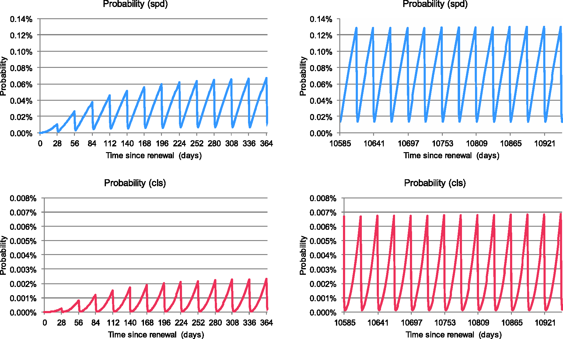
Figure 4 shows how the average probability of the track being in each condition varies throughout its 30-year lifetime. The plots highlight the contribution of the known and unknown conditions to the overall probability of being in each state. They also highlight that the average probability of being in each condition is still changing at the end of the track section’s lifetime, indicating that a steady state has not yet been reached and that the track section’s condition is still generally deteriorating. Figure 5 shows plots of how the probabilities of being in the states where either speed restrictions or line closures should be imposed change during the first and final year of the track section’s lifetime. The 28-day measurement train inspection interval is clearly visible. The probability of the track being in these conditions rises throughout the 28-day inspection interval. As the mean time taken to perform maintenance of an urgent priority is short (0.5 days), the probability of being in these states drops sharply immediately following the inspection. It can be seen clearly in the plots for the first year that the probability of the track section being in these conditions immediately before an inspection is increasing. The same is also true in the final year although the effect is more subtle. This adds to the evidence that the general condition of the track section is still deteriorating at the end of its lifetime. This corresponds to the general worsening of the track section’s condition and the related higher rates of deterioration that are seen following tamping.

Figure 4.

Plots of the changing average probability of the track section being in each condition throughout its 30-year lifetime in the base-case model.

Figure 5.

Probability of the track section being in a condition where either a speed restriction or line closure should be imposed during the first year following renewal and the 30th year following renewal in the base-case model.

When considering the probability of the track section being in a condition and that condition being unknown, the most important conditions to consider are those for which urgent priority maintenance should be performed. Figure 6 considers the probability of the track section being in a condition where speed restrictions should be imposed and that condition is either known or unknown. The plots for the line closure condition exhibit similar features. The measurement train’s inspection interval is again clearly visible. In this case, the probability of knowing that speed restrictions should be imposed is zero until the inspection takes place, and the probability of being in that condition following the inspection soon drops to zero again after the urgent priority intervention has taken place. The corresponding behaviour related to the probability of this condition being unknown can also be seen. This rises between inspections and drops to zero once the inspection has taken place.

Figure 6.

Probability of the track section being in a condition where a speed restriction should be imposed and the condition is either known or unknown during the first year in the base-case model.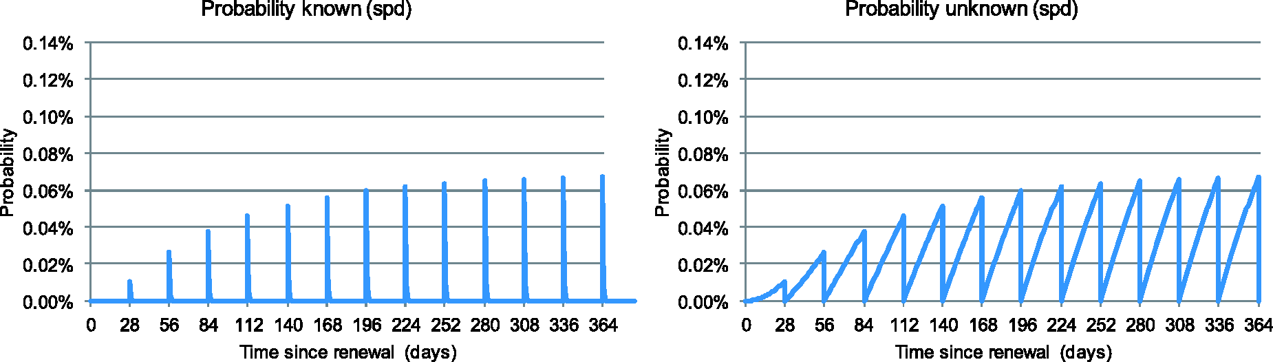

Figure 7 shows how the probability of having performed a certain number of maintenance interventions changes throughout the track section’s lifetime for the base-case model. The general deterioration in the track section’s condition as it ages can be seen from the increase in the probability of having performed a higher number of tamps as the track section ages.

Figure 7.

The changing probabilities of having performed a certain number of maintenance interventions throughout the track section’s lifetime in the base-case model.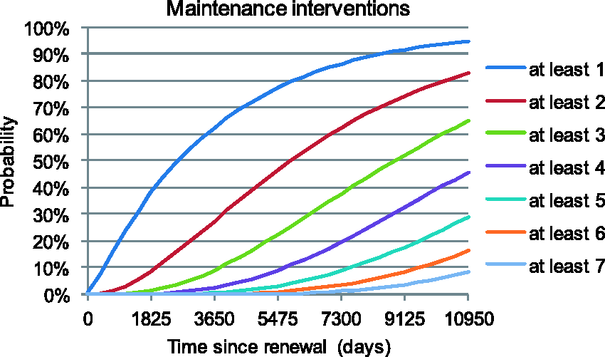

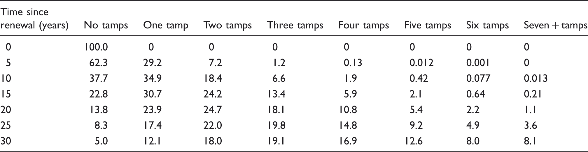
Table 3 presents similar data relating to the probability of having performed an exact number of tamps at 5-year intervals throughout the track section’s lifetime. The gradual deterioration of the track section’s condition can be clearly seen from the increase with time of the probability of a higher number of maintenance interventions having been performed; this increase is in line with the type of behaviour that would be expected in reality. The probability of maintenance having been performed on the track section only exceeds the probability of no maintenance having been performed when the track section has been in use for around 7 years, when the probability of zero tamps falls below 50%. By the time the track has been in use for 16 years following renewal the probability of at least two tamps having been performed exceeds 50% for the first time. Together with information about the costs associated with tamping, this data could be used to predict the likely costs of maintenance throughout the lifetime of the track section.

Table 3.

Probabilities (in per cent) of having performed a certain number of maintenance interventions throughout the track section’s lifetime for the base-case model.

Time since renewal (years)	No tamps	One tamp	Two tamps	Three tamps	Four tamps	Five tamps	Six tamps	Seven + tamps
0	100.0	0	0	0	0	0	0	0
5	62.3	29.2	7.2	1.2	0.13	0.012	0.001	0
10	37.7	34.9	18.4	6.6	1.9	0.42	0.077	0.013
15	22.8	30.7	24.2	13.4	5.9	2.1	0.64	0.21
20	13.8	23.9	24.7	18.1	10.8	5.4	2.2	1.1
25	8.3	17.4	22.0	19.8	14.8	9.2	4.9	3.6
30	5.0	12.1	18.0	19.1	16.9	12.6	8.0	8.1

Investigation of alternative asset management strategies

Table 4 shows how the performance of the track section varies with varying maintenance, inspection and renewal strategies. The base-case model results are presented for comparison.

Table 4.

The average probabilities (in per cent) of the track section being in each condition throughout its lifetime and in the brackets the average time spent in each condition per year for the investigated strategies.

Good	Crit		Spd		Cls
Probability (average days in condition per year)	Probability (average days in condition per year)		Probability (average days in condition per year)		Probability (average days in condition per year)
Known	Unknown	Known	Unknown	Known	Unknown
Base case
96.7 (353)	2.76 (10.1)	0.44 (1.6)	0.002 (0.006)	0.051 (0.186)	0.000,08 (0.0003)	0.001,56 (0.0057)
Level of SD triggering a maintenance request (σcrit)
σcrit = 3·5	97.1 (355)	2.40 (8.8)	0.40 (1.5)	0.002 (0.008)	0.064 (0.232)	0.000,10 (0.0004)	0.001,90 (0.0069)
σcrit = 4	97.6 (356)	1.90 (6.9)	0.36 (1.3)	0.003 (0.012)	0.094 (0.343)	0.000,14 (0.0005)	0.002,75 (0.0100)
Time to perform normal priority maintenance (1/νnorm)
50 days	98.0 (358)	1.49 (5.5)	0.45 (1.6)	0.001 (0.004)	0.029 (0.106)	0.000,04 (0.0002)	0.000,86 (0.0031)
150 days	95.6 (349)	3.86 (14.1)	0.44 (1.6)	0.002 (0.009)	0.070 (0.255)	0.000,11 (0.0004)	0.002,15 (0.0079)
200 days	94.7 (345)	4.82 (17.6)	0.43 (1.6)	0.003 (0.011)	0.086 (0.314)	0.000,14 (0.0005)	0.002,66 (0.0097)
Measurement train’s inspection interval
7 days	97.1 (354)	2.82 (10.3)	0.11 (0.4)	0.002 (0.007)	0.013 (0.046)	0.000,02 (0.0001)	0.000,10 (0.0004)
14 days	97.0 (354)	2.80 (10.2)	0.22 (0.8)	0.002 (0.006)	0.025 (0.093)	0.000,04 (0.0002)	0.000,40 (0.0015)
56 days	96.3 (352)	2.70 (9.9)	0.87 (3.2)	0.002 (0.006)	0.103 (0.375)	0.000,15 (0.0005)	0.006,04 (0.0220)
Renewal period
20 years	96.9 (354)	2.64 (9.7)	0.42 (1.5)	0.002 (0.006)	0.045 (0.165)	0.000,07 (0.0002)	0.001,28 (0.0047)
40 years	96.6 (353)	2.85 (10.4)	0.46 (1.7)	0.002 (0.007)	0.057 (0.207)	0.000,09 (0.0003)	0.001,84 (0.0067)

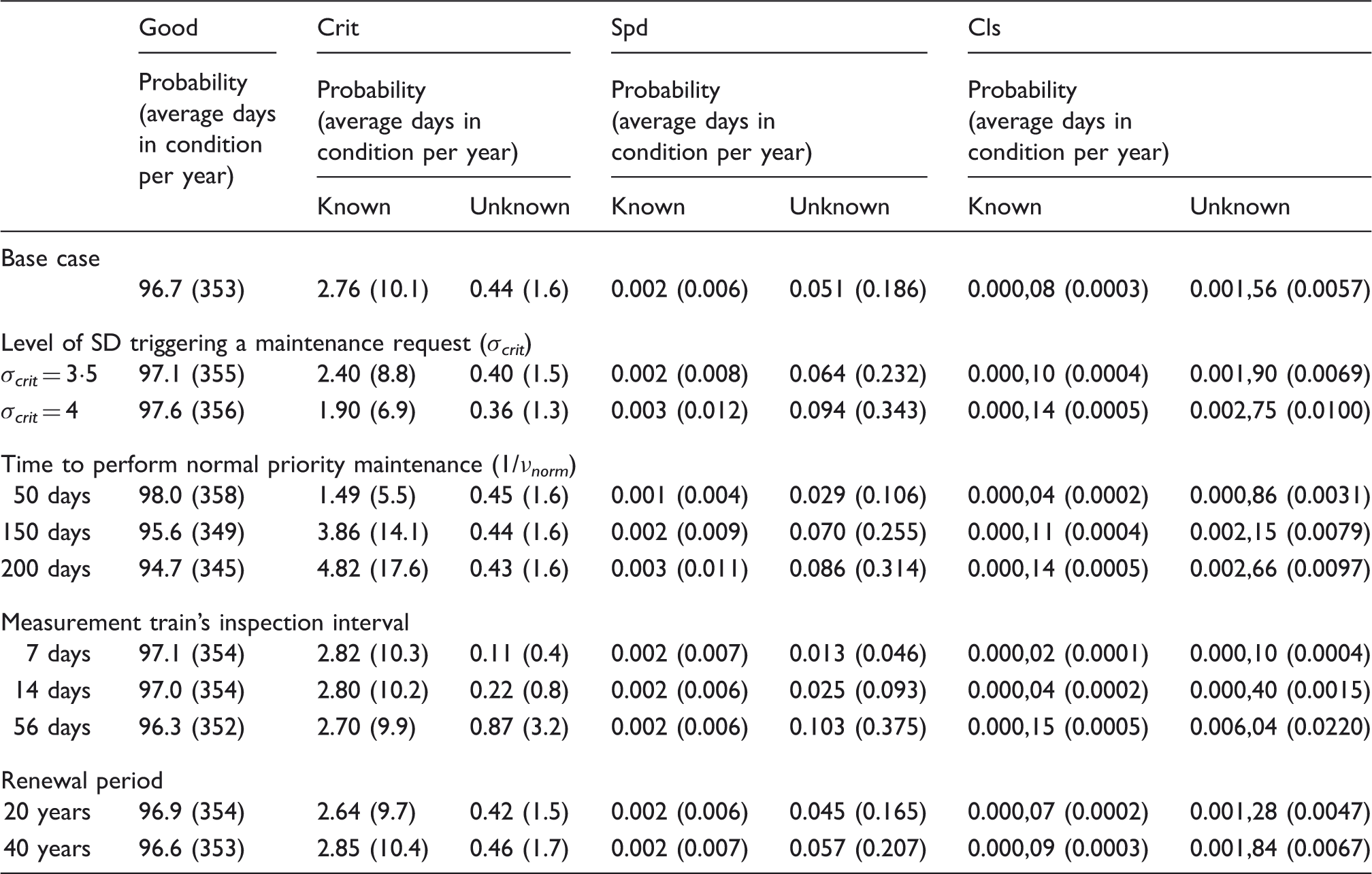
SD at which maintenance is requested

The second section of Table 4 shows the effects of varying the level of SD that triggers a maintenance request, σ_crit. Figure 8 shows how the average probability of the track being in each condition varies throughout the 30-year lifetime as this parameter changes. It can be clearly seen that the probability of being in a condition where either speed restrictions or line closures must be imposed increases as σ_crit is increased. This demonstrates the increased risks that are associated with this strategy. When considering the probabilities of the track section being in the other two conditions (good, crit) the fact that the SD limits that define the boundaries of these conditions have changed must be taken into account. Therefore, the fact that the probability of the track being in the good condition increases as σ_crit increases must be considered in light of the fact that the good track condition also encompasses worse track quality measures as σ_crit increases.

Figure 8.

The changing average probability of the track being in each condition throughout the 30-year lifetime for varying σ_crit.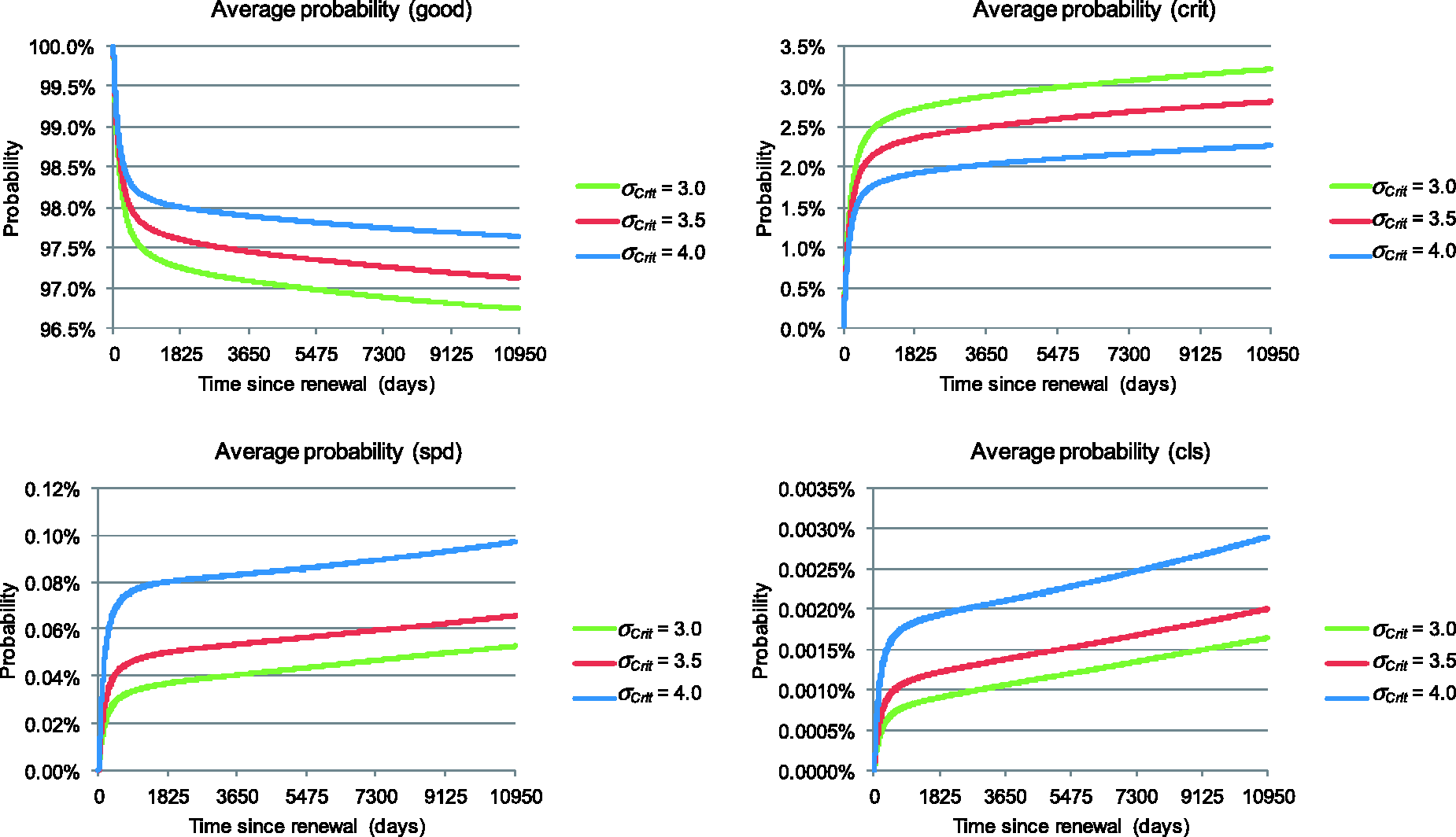

Time to perform normal priority maintenance

The third section of Table 4 and the plots in Figure 9 show the effect of varying the time taken to perform maintenance of a normal priority on the average probability of the track section being in each condition. The time taken to perform this type of routine maintenance is one of the key variables in the asset management strategy, this is because it could correspond to the number of maintenance machines available and the way that they are scheduled to perform the required interventions. As the time taken to perform maintenance is increased the probability of the track section being in a good condition decreases and the probability of it being in the other conditions increases. There is around a threefold increase in the probability of needing to impose speed restrictions or line closures as the maintenance time increases from 50 to 200 days; this will bring an associated increase in the risk of accidents or incidents. Reducing the maintenance time from 100 days for the base- case model to 50 days led to an increase in probability of the track section being in a good condition throughout its lifetime from 96.7% to 98.0%, equivalent to an increase of around 145 days in the time spent in the good condition through the 30-year lifetime. Although this is a significant improvement it would have to be balanced against the extra cost of performing such a maintenance strategy.

Figure 9.

The changing average probability of the track being in each condition throughout the 30-year lifetime for varying time taken to perform maintenance of a normal priority.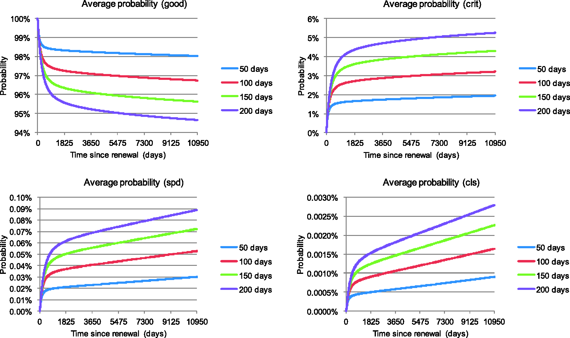

Measurement train inspection interval

The fourth section of Table 4 and the plots in Figure 10 show the effect of varying the measurement train’s inspection frequency on the average probability of the track section being in each condition. There are a number of points to note here. Changing the inspection frequency from once every 28 days in the base-case model to once every 14 days or once every 7 days brings a reduction in the probability of the track section being in a condition that requires either speed restrictions or line closures to be imposed, as would be expected. Increasing the inspection interval to 56 days brings a significant increase in the probability of the track being in these conditions. Looking at the results in more detail, it can be seen that as the inspection interval is increased the proportion of time spent in each condition except that which would require line closures to be imposed, and those conditions being known, decreases. The proportion of time spent in the condition requiring line closures and this condition being known increases. This can be explained by the fact that as the inspection interval increases the track has more opportunity to deteriorate before an inspection can reveal its condition. Therefore, the track is more likely to be in a worse condition by the time the inspection takes place. The proportion of time that the track is in each condition and that condition is unknown increases as the inspection interval increases for all conditions. However, whereas for the other three conditions as the inspection interval doubles the probability of being in the condition and that condition is unknown approximately doubles, for the condition requiring line closures to be imposed the proportion of time is approximately quadrupled. The total time spent in this state is, however, still less than a day over the entire track section’s lifetime.

Figure 10.

The changing average probability of the track being in each condition throughout the 30-year lifetime for varying the inspection interval.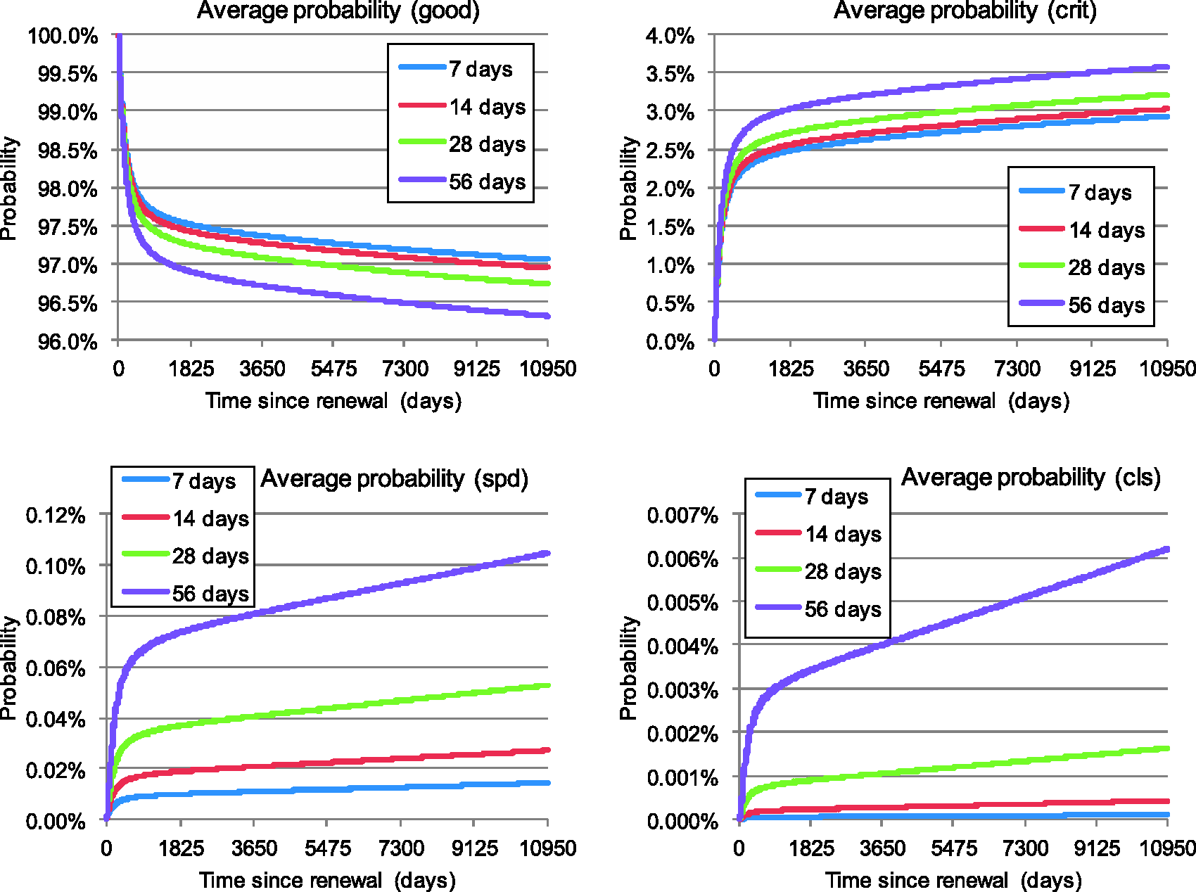

Renewal period

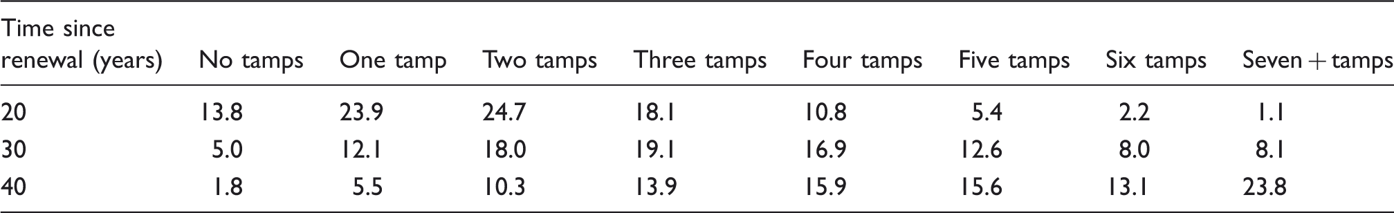
The fifth section of Table 4 shows the effect of varying the track section’s renewal period. Figure 11 illustrates how this change in renewal period affects the average probability of the track section being in the good condition. The proportions of time the track section spends in the other conditions follow similar trends. There is little change in the probability of the track section being in any condition throughout its lifetime. This indicates that the renewal period has little impact on the track section’s performance and suggests that the ballast has generally not suffered significant deterioration in any of the studied lifetimes. This is an interesting result since, as can be seen from Table 5, the distribution of performed maintenance interventions shifts significantly away from the lower numbers of tamps and towards the higher numbers. Since tamping causes the ballast to degrade it might be expected that greater deterioration of the track section’s performance might be seen as the renewal period increases. This might be expected if the renewal period were to be extended further and there was subsequently a greater probability of the track section having been tamped a greater number of times. However, the evidence from this study suggests that choosing a longer renewal period would be a sensible asset management strategy.

Figure 11.

The changing average probability (in per cent) of the track section being in a good condition throughout its lifetime for varying renewal period.

Table 5.

Probabilities of having performed a certain number of maintenance interventions throughout the track section’s lifetime for the three considered renewal periods.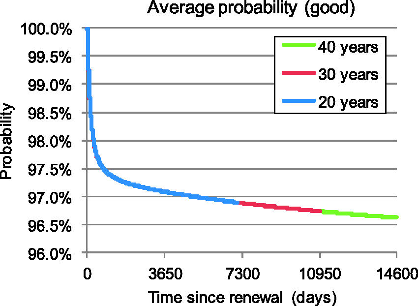

Time since renewal (years)	No tamps	One tamp	Two tamps	Three tamps	Four tamps	Five tamps	Six tamps	Seven + tamps
20	13.8	23.9	24.7	18.1	10.8	5.4	2.2	1.1
30	5.0	12.1	18.0	19.1	16.9	12.6	8.0	8.1
40	1.8	5.5	10.3	13.9	15.9	15.6	13.1	23.8

Summary / conclusions

A Markov model of a 1/8 mile track section has been presented and used to investigate the effects of a number of asset management strategies applied to that track section. The track section’s condition is indicated by a measurement of the vertical alignment of the section and the model incorporates the deterioration of this measurement, maintenance intervention by tamping, inspection by measurement train and the dependence of the rate of deterioration of the track’s condition on the maintenance history.

The model was analysed numerically using a Runge–Kutta algorithm to investigate the effects of varying the following parameters:

the track’s condition that triggers a maintenance request;

the mean time to perform routine maintenance;

the inspection interval at which a measurement train will determine the track’s condition;

the track section’s renewal period.

The model was used to obtain results relating to:

the proportion of time the track spent in certain conditions, classified according to its level of deterioration;

the probability of having performed any number of maintenance interventions on the track throughout its lifetime.

The model could be used to investigate the risk (of delays or accidents) associated with the asset management strategy applied to a track section by looking at the time the track spends in states where speed restrictions or line closures should be imposed but the track is not known to be in that state.

The model could also be used to investigate the cost associated with asset management strategies by considering the costs of the different inspection, maintenance and renewal actions, and the costs associated with penalties imposed when speed restrictions or line closures are applied.

The main drawback of the model is one that is common to many Markov models: its size. Although the presented model is not prohibitively large, a similar model that incorporated other maintenance options such as stoneblowing, or a number of track sections rather than just one, would exhibit a state-space explosion that might make the analysis difficult to perform.

The model could also be extended to account for other aspects of deterioration such as lateral misalignment or wear of the rails and related maintenance such as rail grinding. However, the addition of other aspects such as these may also lead to state-space explosion and a prohibitively large model.

The model’s main advantage is its relative simplicity. Despite this simplicity it can be used to draw a number of important conclusions about the impact of an asset management strategy on a single track section.