Sage Journals: Discover world-class research

Abstract

This study investigates the effects of elbow on the transition and development of multiphase flow using computational fluid dynamics modelling techniques. The Eulerian - Multifluid VOF model coupled with an Interfacial Area Transport Equation has been employed to simulate air-water two-phase flow in a pipe with two standard 90 degree elbows mounted in series. Turbulence effects were accounted for by the RNG k-ε model. The effects of separation distance on two-phase flow development have been studied for initial slug and churn flow regimes. Computational fluid dynamics simulation results of phase distribution and time series of void fraction fluctuations were obtained and they showed good agreement with available experimental data. The results show that for initial slug flow regime, there is no flow regime transformation upstream and downstream of the two elbows. While at initial churn flow regime, flow regime transformation occurs at different sections of the flow domain before and after the two elbows. It was noticed that irrespective of the flow regime, the amplitudes and frequencies of void fraction fluctuation become smaller as the fluid flows along the pipe. Changes in the separation distance between the two elbows have larger effects on the flow at churn flow regime.

Keywords

Multiphase flow elbows computational fluid dynamics (CFD)double elbows/bends churn flow slug flow

Introduction

Two-phase gas-liquid flow occurs in many industries such as chemical, petroleum, food and drink, processing and manufacturing. Two-phase flow is characterised by differences in the interface between phases leading to different two-phase flow regimes. Gas dominant flow regimes such as pseudo slug, churn and annular are the most commonly observed flows in industry and many experimental and numerical techniques have been applied to study the features of these types of flows.^1–11 Many of these studies have focused on simple geometries where fluids flow through a vertical or horizontal pipe or through a single elbow. However due to the availability of space and economics of design, there is a need for using complex piping systems such as multiple bends pipe, and U-bend to transport fluids. The knowledge of two-phase flow phenomenon in bends and its development downstream of bends is important in many industrial applications. In addition to oil-gas processing platforms where two-phase flow undergoes several changes of directions due to bends under limited space, Zhao et al.² have shown two specific examples of two-phase flow at multiple bends (i) fire reboiler with serpentine tubing and (ii) a novel combined bend/T-junction phase separator.

Two-phase flow regimes in vertical and horizontal pipes are quite different. In vertical pipes, annular, churn, slug and bubbly flows are observed, while dispersed bubble, slug, stratified and annular flows are observed in horizontal pipes.³ Flow regimes can change rapidly at the bends where the flow changes direction from vertical to horizontal or horizontal to vertical orientation.

The behaviour of two-phase flow upstream and downstream a sharp return elbow was studied using capacitance sensors by Kerpel et al.¹² with an elbow of 1 mm radius of curvature and 0.008 m internal diameter. R134a refrigerant was employed while mass flux and vapour liquid void fraction were varied between 200–400 kg/m²s and 0 to 1 respectively. To determine the effects of elbow, eight capacitance sensors were positioned at different locations upstream and downstream of the elbow to extract a series of void fraction data. In their experiment, flow regimes before the bend were slug, intermittent and annular flows. It was observed that in the pipe section downstream of the bend, no bend effect is evident for slug flow but there were ripples and disturbances at the phase interface. In intermittent and annular flows on the other hand, no visually detectable effects on the flow behaviour due to the elbow were evident. It was also concluded that the disturbance and ripple effects due to the elbow stretches out to at least 21.5 tube diameters downstream of the elbow. Abdulkadir et al.¹³ also reported observations from the study of two-phase air-water churn-annular flow in a large diameter vertical 180 degrees return elbow using electrical conductance technique. The elbow has a diameter of 0.127 m and a curvature ratio (R/D) of 3. Superficial velocities of air were ranged from 3.5 to 16.1 m/s and those for water from 0.02 to 0.2 m/s. The flow patterns were identified to be within the slug – churn transition region using Probability Density Function (PDF) profiles of the time series of the mean film fractions. The flow pattern upstream of the elbow was confirmed to be churn flow while in the downstream, the liquid was observed to drain to the bottom of the elbow due to gravity effects, the gas was at the centre of the pipe leading to annular flow pattern. Asgharpour et al.¹ also performed experiments to investigate churn/annular and pseudo-slug flow before and after pipe elbows in a 76.2 mm pipe. Wire mesh sensor (WMS) was used to determine the void fraction distributions in the upward-vertical orientation before the elbow and the horizontal orientation after the elbow for 11 m/s and 0.1 m/s gas and liquid velocities. They observed that the flow transitioned from annular – churn in the vertical section to a wavy stratified flow in the horizontal section. Vieira et al.¹⁴ investigated the effect of 90° standard elbow on horizontal gas–liquid stratified and annular flow characteristics using dual wire-mesh sensors. The horizontal test section was a 0.0762 m ID, 18 m long pipe and it generated stratified-wavy and annular flows. Two 16 × 16 wire-mesh configuration sensors were positioned at 0.9 m upstream and 0.6 m downstream of the elbow, and the experiments were conducted at superficial liquid velocities of 0.03 m/s and 0.2 m/s while superficial gas velocities ranged from 9 m/s to 34 m/s. The cross-sectional averaged void fraction time series showed similar structures in the upstream and downstream locations for stratified and annular flows. It was also reported that wave instability is the most notable feature of the stratified to slug transition in both upstream and downstream locations of the elbow, the cross-sectional time averaged void fraction values slightly increased after the 90° horizontal elbow and in the downstream section more liquid is in the perimeter of the pipe and waves are smaller as compared with the upstream conditions Zhao et al.² has reported an experimental study of two-phase flow regime transition in a double-bend pipe line. Zhao et al.² reported experimental investigations concerning gas-liquid two-phase flows in two 90 degree bend in series with fixed separation distance. The flow direction was vertical to horizontal then horizontal to horizontal configuration in their study. Phase distribution within the elbows and downstream of the elbows were studied via capacitance measurements. Their results showed that flow transformation occurred in two phase flows due to secondary flows as well as gravity effects at the bend. PDF analysis showed clear evidence that stratified plug, wavy and slug flows were developed in the horizontal section after the bend, while slug and churn flows occurred in the upstream of the elbow when the gas and liquid superficial velocities were 0.3 to 4 m/s and 0.21 to 0.91 m/s respectively. Further analyses showed that due to the bend, for a liquid superficial velocity of 0.38 m/s and the gas superficial velocity of 0.05 m/s, upstream bubbly flow transformed into stratified flow downstream of the elbow while at a liquid superficial velocity of 0.38 m/s and gas superficial velocity of 0.71 m/s the upstream slug flow transformed into plug flow after the elbow with large gas bubbles separated by a liquid layer. As the two-phase flow passed around the bend to the horizontal sections, the liquid phase drained to the bottom of the pipe due to the effect of gravity and transitioned into stratified flow which remained dominant across the horizontal sections. It was also observed that the minimum distance necessary for the development of the flow after the 90° bend is between 10 to 50 D from the bend depending on the flow rates.

The above literature review shows that there exists a gap in knowledge in the understanding of two-phase flow transition under multiple bends with different separation distances. These pipe configurations are very common in offshore oil and gas processing platforms, refineries, food processing plant and can be used in designing innovative bend phase separator. This paper aims to provide a fundamental understanding of two-phase flow transitions in multiple pipe bends.

The transient nature of gas-liquid two-phase flows still remains a key challenge in multiphase flow studies both experimentally and numerically and CFD can provide vital flow information and interactions between flow phases. Volume of Fluid (VOF) model is a widely used approach for simulating multiphase flows^4,10,15–19 where there is distinct interface between phases such as stratified or slug flow regimes. In the present study, a Multifluid VOF model which is a Eulerian-Eulerian model with an added interface sharpening model from volume of fluid, has been employed in order to investigate the development of multiphase flows before and after the elbows in double elbow (vertical upward – horizontal - vertical downward) geometries for various separation distances.

Numerical modelling

Two-fluid Eulerian-Eulerian two-phase model has been utilised in the present simulations. In order to capture the distinct interface between liquid and gas phases especially in the slug and churn flow regime an additional interface capturing method has been used which is known as Multifluid-VOF model as known in Ansys Fluent. To account for different bubble sizes and their bubble breakage and coalescence within the flow without resolving to details of bubble size distribution such as in population balance model, a simplified modelling assumption of an Interfacial Area Concentration (IAC) transport equation was incorporated in this hybrid model.

Eulerian-Eulerian two-phase flow modelling

Continuity equation

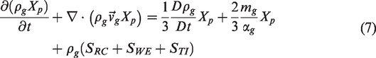
The continuity equation for the phases are

\frac{\partial ρ_{i} α_{i}}{\partial t} + \nabla \cdot (α_{i} ρ_{i} {\vec{v}}_{i}) = 0

(1)

\sum_{q}^{n} α_{i} = 1

(2)

Where $α_{i}, ρ_{i} and {\vec{v}}_{i}$ are the volume fraction, density and velocity of the individual phases.

Momentum equation

The momentum equation for the phases are

\frac{\partial (α_{i} ρ_{i} {\vec{v}}_{i})}{\partial t} + \nabla \cdot (α_{i} ρ_{i} {\vec{v}}_{i} {\vec{v}}_{i}) = - α_{i} \nabla p + \nabla \cdot τ_{i} + α_{i} ρ_{i} \vec{g} + \vec{F_{i j}}

(3)

Where P and $τ_{i}$ are the pressure and stress-strain tensor of the individual phases, $\vec{g}$ is acceleration due to gravity and $\vec{F_{i j}}$ is the interfacial force between the phases.

The general form of the interfacial force $\vec{F_{i j}}$ from equation (3) is expressed as

\vec{F_{i j}} = K_{i j} ({\vec{v}}_{i} - {\vec{v}}_{j})

(4)

where, $K_{i j}$ is the interphase momentum exchange co-efficient between the phases. In the Eulerian-Eulerian two-phase flows, the second phase is treated as bubbles and the interphase exchange coefficient is given by

K_{i j} = \frac{ρ_{i} f}{6 τ_{i}} X_{p}

(5)

where, $X_{p}$ is the interfacial area concentration, $f$ is the drag co-efficient and $τ_{i}$ is the particle relaxation time given by

τ_{i} = \frac{ρ_{i} d_{i}^{2}}{18 μ_{j}}

(6)

Schiller and Naumann²⁰ model is used to calculate drag coefficient $f .$

Interfacial area concentration

The solution of interfacial area concentration allows the inclusion of bubble diameter distribution and coalescence/breakage effects within limited computational resources.

The transport equation for interfacial area concentration, IAC, is given as

\frac{\partial (ρ_{g} X_{p})}{\partial t} + \nabla \cdot (ρ_{g} {\vec{v}}_{g} X_{p}) = \frac{1}{3} \frac{D ρ_{g}}{D t} X_{p} + \frac{2}{3} \frac{m_{g}}{α_{g}} X_{p} + ρ_{g} (S_{R C} + S_{W E} + S_{T I})

(7)

where $X_{p}$ is the interfacial area concentration and $α_{g}$ is the gas volume fraction. The first two terms on the right hand are the gas bubble expansion due to compressibility and mass transfer, $m_{g}$ is the mass transfer rate into the gas phase per unit mixture volume. $S_{R C}$ and $S_{W E}$ are coalescence sink terms due to random collision and wake entrainment respectively. $S_{T I}$ is the breakage source term due to turbulent impact. The source and sink terms are accounted for with the Hibiki-Ishii model.²¹ The interfacial area concentration is coupled with the momentum equation via the interfacial force(s) in equation (5).

Multi-Fluid VOF

In slug and churn flow situations, there is a distinct and sharp interface between the liquid and gas phase. This sharp interface has been captured in the present study using a combination of volume of fluid method with Eulerian-Eulerian model explained earlier. At the interface of two phases based on the value of calculated volume fraction, a special interpolation treatment is applied to the cells that lie near the interface between the two phases to capture the shape interface using the High Resolution Interface Capturing (HRIC) scheme.²²

Turbulence modelling

In the present study, turbulence is represented by mixture turbulence concept where turbulence is calculated using fluid mixture properties and was accounted for by using the RNG k-ε model.²³ The RNG k-ε transport equations are:

Kinetic Energy, $k$

\frac{\partial}{\partial t} (ρ k) + \frac{\partial}{\partial x_{i}} (ρ k {\vec{v}}_{i}) = \frac{\partial}{\partial x_{j}} (α_{k} µ_{eff} \frac{\partial k}{\partial x_{j}}) + G_{k} - ρ Ɛ

(8)

Dissipation rate, Ɛ

\frac{\partial}{\partial t} (ρ Ɛ) + \frac{\partial}{\partial x_{i}} (ρ Ɛ {\vec{v}}_{i}) = \frac{\partial}{\partial x_{j}} (α_{Ɛ} µ_{eff} \frac{\partial Ɛ}{\partial x_{j}}) + C_{1 Ɛ} \frac{Ɛ}{k} (G_{k}) - C_{2 Ɛ} ρ \frac{Ɛ^{2}}{k} - R_{Ɛ}

(9)

$G_{k}$ is the generation of turbulence kinetic energy due to the mean velocity gradients. $α_{k}$ and $α_{Ɛ}$ are the inverse effective Prandtl numbers for $k$ and $Ɛ$ respectively. $C_{1 Ɛ}$ and $C_{2 Ɛ}$ are 1.42 and 1.68, $µ_{eff}$ is the effective viscosity. The effective viscosity is given by

μ_{eff} = μ + μ_{t} and μ_{t} = \frac{ρ C_{μ} k^{2}}{Ɛ}

(10)

Where, $C_{μ} = 0.085$ .

RNG k-ε is more accurate and reliable for a wider class of flows. They are also more responsive to the effects of rapid strain and streamline curvature and thus is suitable for flow through bends²³

R_{ε} = \frac{C_{µ} ρ η^{3} (1 - η / η_{0})}{1 + β η^{3}} \frac{ε^{2}}{k}

(11)

and

η = \frac{S k}{Ɛ}; η_{o} = 4.38, β = 0.012

(12)

where, $S$ is strain rate of fluid flow.

Solver control/numerical schemes

Ansys Fluent version 19.1 has been used for providing the numerical solutions of the governing equations of mass, momentum, phase volume fraction and turbulence. In this study, three dimensional (3-D) transient simulations were performed with the assumption that the liquid and gas phases were incompressible with no mass transfer between them. Momentum and turbulence equations are discretised using the upwind scheme and pressure and velocity equations are coupled with phase-coupled SIMPLE algorithm. Discretised algebraic equations use the under-relaxation factor of 0.3 for pressure, momentum and interfacial area concentration equations; 0.5 for volume fraction and 0.6 for turbulence kinetic energy and energy dissipation rate. The governing equations are solved in transient scheme with a time step of 0.001 s. Solutions are deemed converged when the residuals of all equations reach below 10⁻⁶. It took between 10 to 20 iterations to reach convergence in each time step.

Flow domain

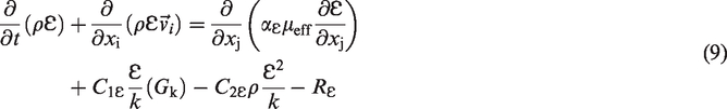
The single elbow 3-D geometry in Figure 1(a) was modified to accommodate a second elbow as shown in Figure 1(b), and the normalized separation distance (L/D) between the two elbows mounted in series are 0, 5, 10, 15 and 20. The 3-D computational geometry in Figure 1(a) is similar to that of Parsi et al.,²⁴ it consists of 3 m vertical and 1.9 m horizontal pipes, upstream and downstream of a standard 90-degree elbow respectively and the flow of fluids is from upward vertical to horizontal. Pipe diameter and the radius of curvature of elbow are 0.0762 m and 1.5 respectively.

Figure 1.

Computational domains.

Boundary conditions

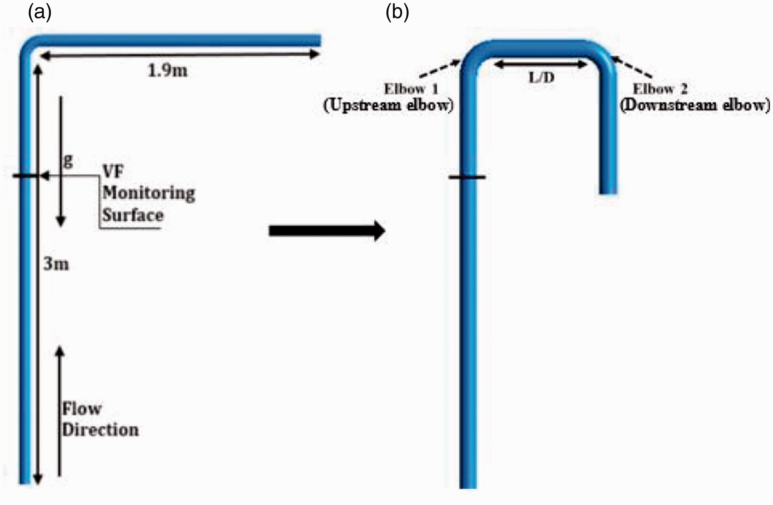
Velocity-inlet and pressure-outlet boundary conditions have been set at the inlet and outlet respectively (see Figure 2). Standard log-law of the wall was used at the wall. Turbulence intensity of 5% was set at the inlet. To aid faster flow development, the pipe inlet surface was split into two as shown in Figure 3 similar to CFD simulation of Parsi et al.²⁵ Gas was introduced into the domain via the middle of the inlet (red patch) while the liquid was introduced circumstantially (blue patch). The liquid and gas phases were introduced into the domain based on the velocities obtained from equations (13) and (14), respectively. The whole domain was initially filled with the liquid phase at zero velocity.

V_{inlet - gas} = \frac{V_{sg} * A_{p}}{A_{g}}

(13)

V_{inlet - liquid} = \frac{V_{sl} * A_{p}}{A_{l}}

(14)

Figure 2.

Boundaries of computational domain.

Figure 3.

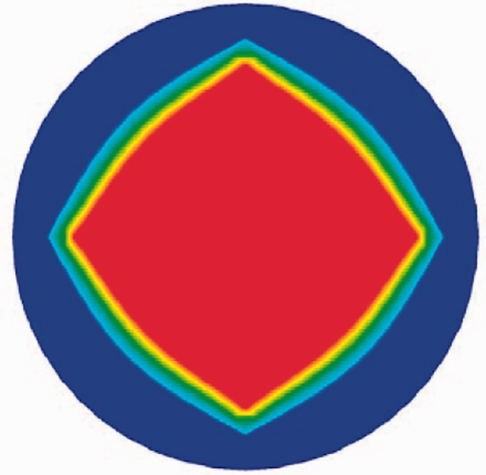
Injection of the phases via the inlet – red and blue indicates air and water respectively.

Where, $V_{s g}$ and $V_{s l}$ are superficial gas and liquid velocities, $A_{p}$ is the area of the pipe and $A_{g}$ and $A_{l}$ are inlet areas of gas and liquid.

Mesh/grid generation

A structured grid was generated across the flow domain as shown in Figure 4. Three different grids were considered in conducting a mesh sensitivity analysis in this study comprises of 80000 (mesh 1), 105000 (mesh 2) and 181608 (mesh 3) cells. Figure 5 shows the cross-sectional slices of the three grids in the perpendicular direction of the flow.

Figure 4.

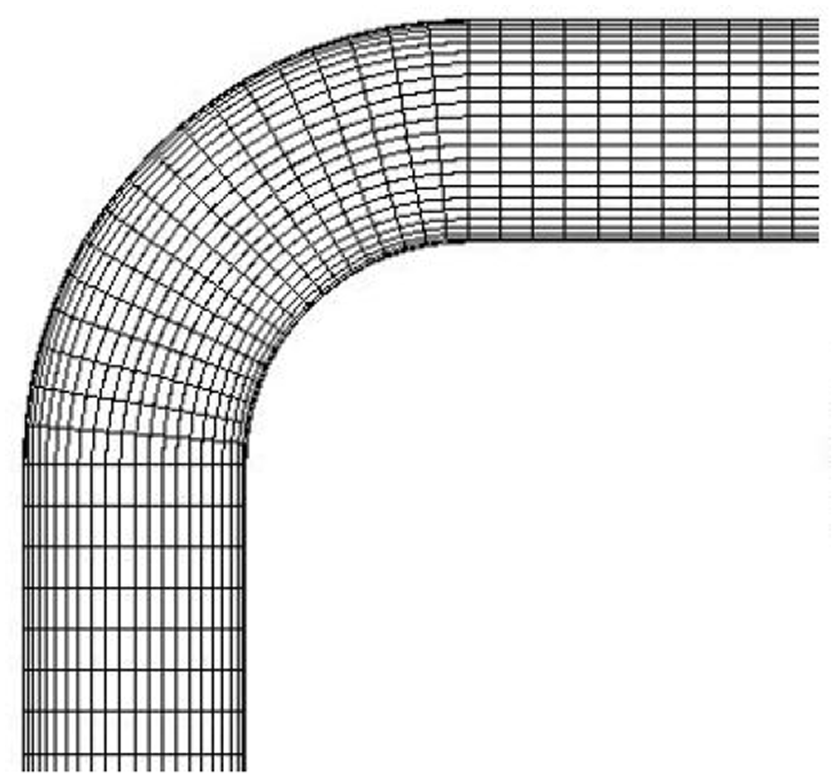
Part of meshed flow domain.

Figure 5.

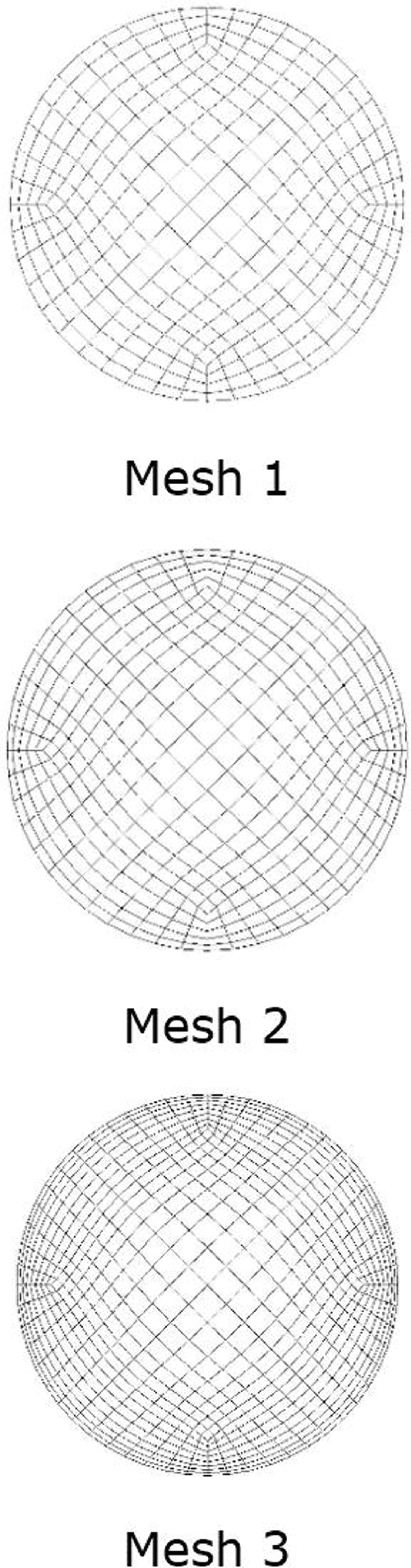
Cross-sectional slices of the different grids employed.

Flow conditions

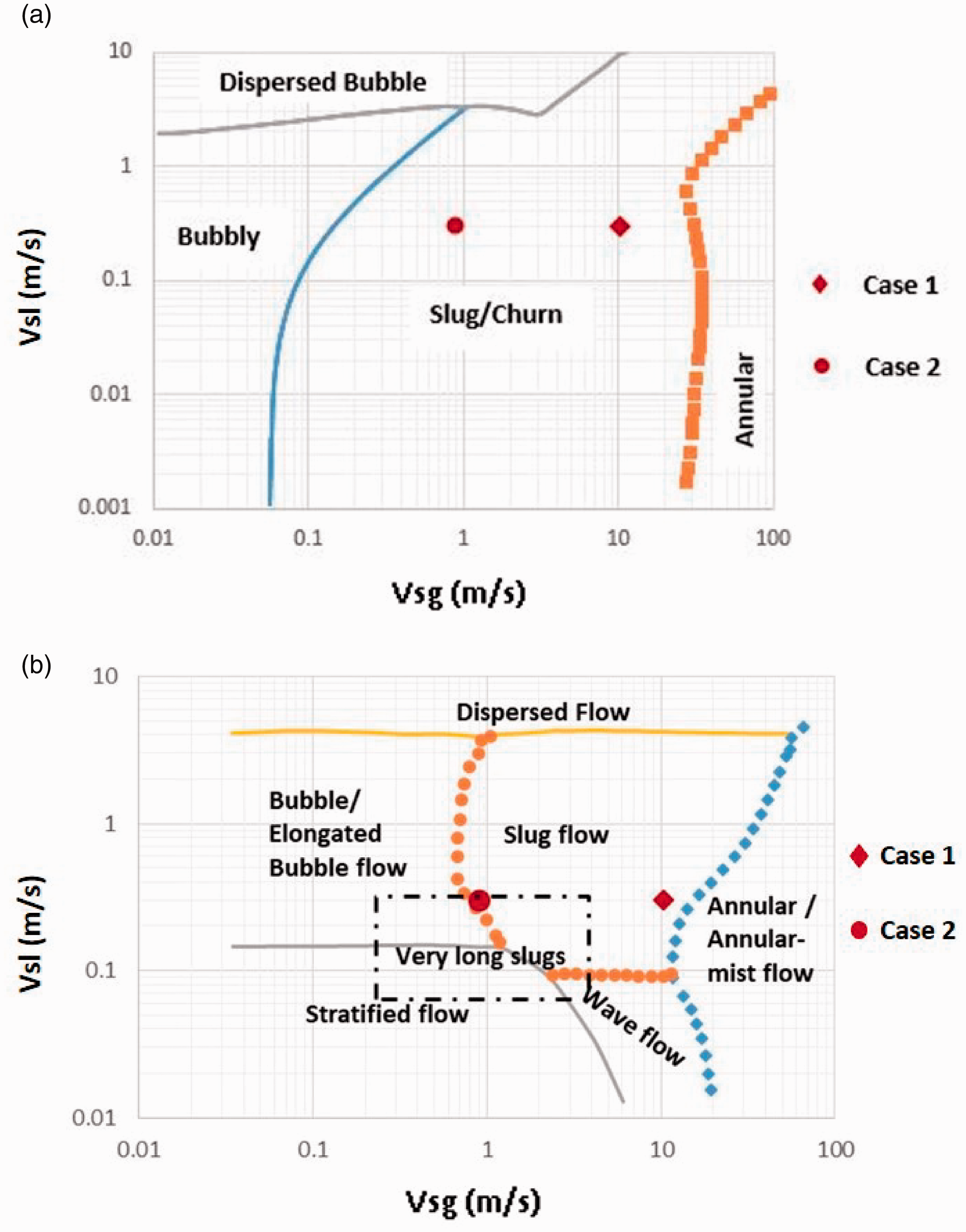
Simulations have been carried out for single and double bend pipes for two flow conditions where the superficial liquid velocity ( $V_{s l}$ ) was kept constant at 0.3 m/s while the superficial gas velocities ( $V_{s g}$ ) were 0.9 m/s and 10.3 m/s. Air and water were the gas and liquid phases respectively in the present study. These flow conditions fall within slug/churn flow regimes in vertical pipe as shown in Figure 6(a) according to the vertical flow regime map of Liu et al.,²⁶ however in horizontal pipe these flow conditions fall near the boundary of elongated bubble and slug; and slug and annular flow regime as in Figure 6(b) (Kadiri²⁷ flow regime map).

Figure 6.

Flow conditions on flow pattern map: (a) vertical pipes; (b) horizontal pipes.

Results and discussion

Mesh Sensitivity study

Figure 7 shows the effect of the grid size on predicted cross-sectional averaged void fraction for the flow condition of superficial gas velocities ( $V_{s g}$ ) of 10.3 m/s and superficial liquid velocity ( $V_{s l}$ ) of 0.3 m/s at 1 m upstream of the elbow. Though it is difficult to ascertain mesh independency from the Figure 7, time averaged void fraction and its standard deviation have been compared with the experimental data of Parsi et al.²⁴ Table 1 shows the mean void fraction and standard deviation of the times series of cross-sectional averaged void fraction. Meshes 1 and 2 produced similar averages while Mesh 3 produced an average higher than the experimental data. The standard deviation however shows that Mesh 2 produced fluctuation data that are much closer to the experimental data of Parsi et al.²⁴ than Meshes 1 and 3. Mesh 2 was therefore selected for all other simulations.

Figure 7.

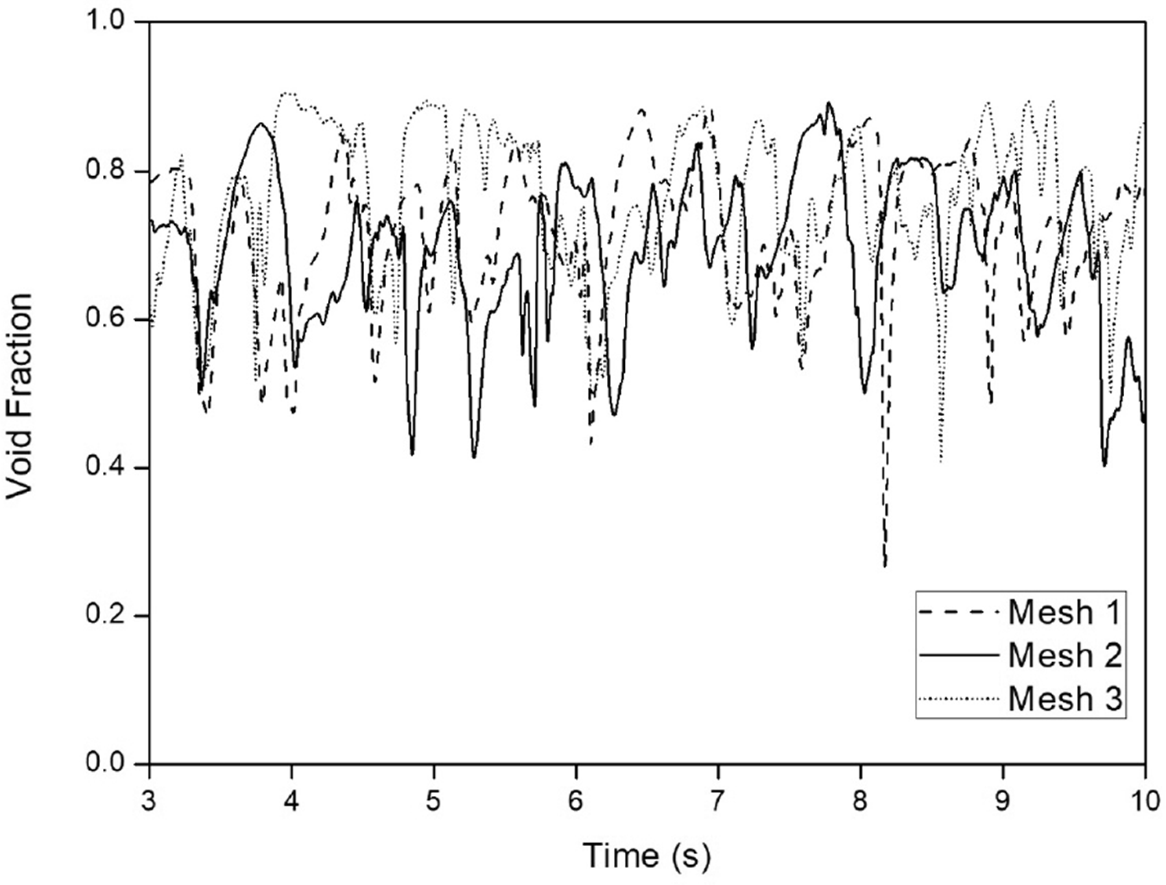
Effect of grid size on the cross-sectional averaged void fraction time-series 1 m before the elbow.

Table 1.

Comparison of experimental and simulation data.

	Experiment²⁴	Mesh 1	Mesh 2	Mesh 3
Mean	0.74	0.72	0.72	0.76
SD	0.10	0.12	0.11	0.12

Single elbow validation

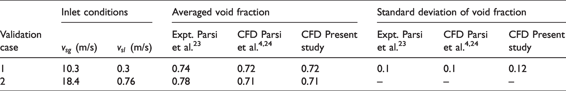
The predicted area-averaged volume fraction at 1 m upstream of the bend has been compared with both previously reported experimental and simulation data of Parsi et al.^24,25 for two different flow conditions of superficial gas velocity of 10.3 m/s and superficial liquid velocity of 0.3 m/s and superficial gas velocity of 18.3 m/s and superficial liquid velocity of 0.76 m/s.

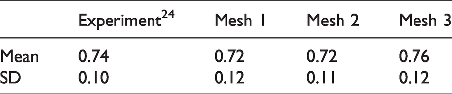
Figure 8 shows the comparison of the time series of cross-sectional averaged void fraction for single elbow for superficial gas velocity ( $V_{s g}$ ) of 10.3 m/s and superficial liquid velocity ( $V_{s l}$ ) of 0.3 m/s with the experimental and numerical data of Parsi et al.^4,24,25 The time series of void fraction is characterised by a higher value of 0.9 characterising gas cores with some liquid droplets and then a lower value of 0.2 characterising the periodic passage of liquid structures. The lowest drop in amplitude in the experimental and numerical data of Parsi et al.^24,25 are 0.24 and 0.33 respectively, while the lowest volume fraction drop in the present study is 0.37. The highest amplitude on the other hand are 0.95 for experimental and CFD data of Parsi et al.^24,25 and 0.9 in the present study.

Figure 8.

Cross-sectional averaged void fraction time series of Vsg = 10.3 m/s and Vsl =0.3 m/s.

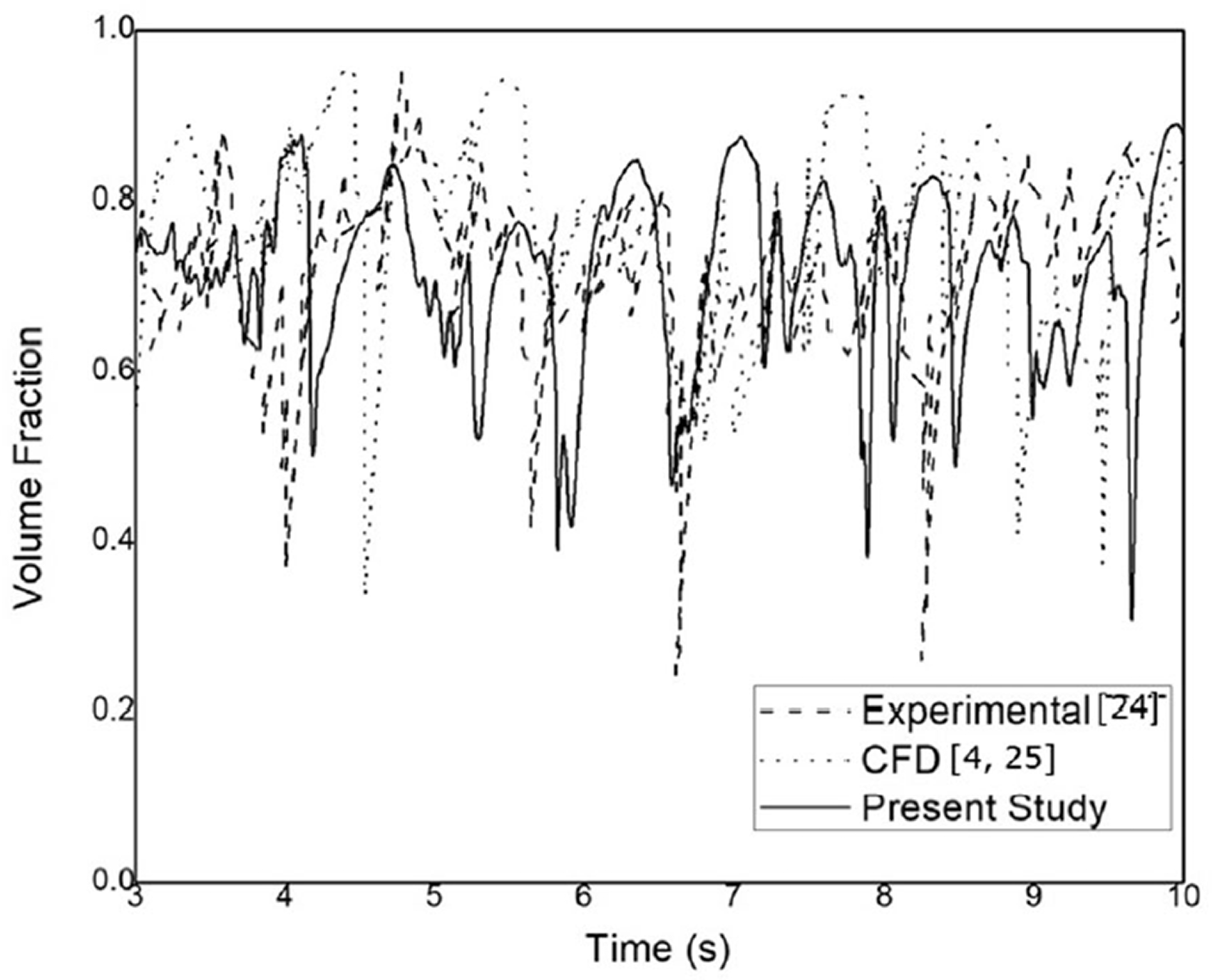
Furthermore, Table 2 shows the mean and standard deviation of the time series of cross-sectional averaged void fraction and its standard deviation of the present study compared with available numerical and experimental data. It is evident from Table 2 that the present simulations reproduce CFD prediction of Parsi et al.^4,25 for both mean and standard deviation of the transient void fraction for two different flow regimes and produce similar discrepancies with experimental data as Parsi et al.^4,25 prediction. Based on this confidence level, the model was extended to multiphase flow analyses in the double elbow geometries of interest.

Table 2.

Validation of CFD modelling.

Validation case	Inlet conditions		Averaged void fraction			Standard deviation of void fraction
Validation case	$v_{s g}$ (m/s)	$v_{s l}$ (m/s)	Expt. Parsi et al.²³	CFD Parsi et al.^4,24	CFD Present study	Expt. Parsi et al.²³	CFD Parsi et al.^4,24	CFD Present study
1	10.3	0.3	0.74	0.72	0.72	0.1	0.1	0.12
2	18.4	0.76	0.78	0.71	0.71	–	–	–

Multiphase flows in double elbow geometries

Two different gas velocities in the slug/churn multiphase flow region were studied at a constant liquid velocity. Superficial gas velocities were 0.9 and 10.3 m/s while superficial liquid velocity was kept constant at 0.3 m/s. The normalised separation distance (L/D) between the upstream and downstream elbows (Elbows 1 and 2) was varied from 0 to 20 at intervals of 5. Supplementary Figure 9 shows the position of four (4) monitoring surfaces for which the data considered in this study were extracted. For L/D of 0, Locations 1 and 2 are not available.

Flow visualisation

Supplementary Figure 10(a) and (b) show the contour plots of the cases 1 ( $V_{s g}$ = 10.3 m/s; $V_{s l}$ = 0.3 m/s) and 2 ( $V_{s g}$ = 0.9 m/s; $V_{s l}$ = 0.3 m/s) studied after 10 s of simulation run time when the normalized separation distance is 0, the figures show that the flow patterns in the vertical upstream pipe before Elbow 1 are characterised by churn and slug flows respectively. Churn flow has the attributes of both slug and annular flows, however, there are no clear boundaries between the liquid and gas phases but there is the presence of waves and discontinuous gas cores. Some authors consider this type of flow to be fundamentally annular flow in nature with large disturbance waves carried by the gas flow^28,29 and just as in this study, huge waves in churn flow was also observed by Parsi et al.^4,24 and Riva and Col.¹⁰ Unlike the churn flow, there are clear and defined boundaries between the liquid and gas phases in Case 2 (Supplementary Figure 10(b)). The small bubbles between the two Taylor bubbles in Supplementary Figure 10(b) were also observed by previous researchers.^28–30

As the normalised separation distance increases, the multiphase flow in the horizontal section after Elbow 1 (upstream elbow) was analysed to study the flow development and transition towards and after Elbow 2 (downstream elbow). Supplementary Figure 11(a) shows the contour plots of the averaged void fraction across a symmetric plane of the flow at 10 s when superficial gas velocity ( $V_{s g}$ ) is 10.3 m/s and superficial liquid velocity ( $V_{s l}$ ) is 0.3 m/s. It is observed that in the churn flow, after the first elbow, gas and liquid separates out into wavy stratified flow. As the normalized separation distance increases, a slight but notable difference is observed in the flow development in the horizontal section (between the elbows), when L/D is 0 it is observed that the liquid phase flows through the elbows more as a thin film pushed towards the extrados of Elbow 2 (downstream elbow), this is due to the effects of secondary flow and centrifugal force in the elbow. When the normalized separation distance (L/D) increased to 5, the presence of liquid phase becomes more pronounced in the horizontal section between Elbows 1 and 2 and the effects of secondary flow and centrifugal forces diminished as the separation distance between elbows increased. At this stage, gravity effects on the flow become more significant with the fluid with the higher density (liquid phase) flowing at the bottom of the pipe and the lighter gas phase moving at the top of the liquid phase. At the normalised separation distance of 10, 15 and 20, after an equivalent normalised distance of about L/D of 15, the liquid phase is observed to be settled and flowing at an almost uniform level at the bottom of the horizontal pipe section. After Elbow 2 (downstream elbow), secondary flow effects on the flow become significant again, the liquid and gas phases are seen to flow at either end of the downstream vertical pipe section. Supplementary Figure 11(b) shows instantaneous flow development across the 4 monitoring surfaces in the flow domains across all L/Ds, it can be seen that in the vertical section before Elbow 1, the flow behaves more like annular flow as stated with the presence of a gas core while at the outlet of upstream elbow (Elbow 1) as the flow navigates into the horizontal section, the phases separate into a stratified flow due to gravity effects. As shown in Figure 6, the flow regime in horizontal pipe should be slug, the secondary flow created at the elbow enhanced flow separation leading to stratified flow in the horizontal section after the bend.

Supplementary Figure 12(a) shows the contour plots of the averaged void fraction of the flow in the symmetrical plane across the flow domains at 10 s for the case of gas superficial velocity of 0.9 m/s and liquid superficial velocity of 0.3 m/s. Although the contour plots show the flow to be stratified in the horizontal section, however, the liquid content at different sections of the pipe occupies more than 50% of the flow domain and in some sections the whole domain, thereby separating the gas phase into pockets. These features are indicative of slug flows in horizontal pipes where the liquid slug at the bottom of the pipe bridges the gas phase at different sections to form gas pockets known as the Taylor Bubbles. An increase in the normalized separation distance aided better development and separation of the flow, it is seen that after a separation distance (L/D) of 5, the presence of the liquid slug and elongated Taylor bubble becomes obvious. Supplementary Figure 12(b) shows the instantaneous flow development across the four (4) monitoring surfaces in the flow domain across all L/Ds, the gas core is indicative of the Taylor bubble passing through at the particular instance on the monitoring surface before Elbow 1.

Quantitative analysis of two-phase flow behaviours due to double bend

The two-phase flow development due to double bends has been analysed through area-average void fraction along the length of the pipe as well as probability density function and power spectral density function.

Statistical analysis of the behaviour of void fraction is one method that can also be used to further ascertain flow patterns in double bend pipe arrangement. According to Costigan and Whalley²⁸ and Lowe and Rezkallah²⁹ every two-phase flow pattern exhibit a specific probability density function (PDF) of void fraction. Churn flow is characterized by a PDF curve with a single broad peak at high void fractions and a broad tail at the low void fractions. The single peak at high void fraction is indicative of the flow’s proximity to annular flow and the broad tail represents the passage of unstable slugs. According to Lowe and Rezkallah,²⁹ a typical PDF curve of churn flow is between an average void fraction of 0.7 and 0.9. In slug flow on the other hand, the PDF of time series averaged void fraction has two peaks, one at the low void fractions and another at the higher ones. These peaks represent the periodic passage of the two specific features of slug flows; the Taylor bubble at high void fractions and liquid slug at low void fractions. In this study, the Ksdensity function of MATLAB was used to generate the Probability Density Function (PDF) profiles of the times series of average void fractions. Power spectral density (PSD) of the time domain signals of the cross-sectional averaged void fractions is another important parameter to ascertain two-phase flow characteristics. Power Spectral Density (PSD) shows the strength of the variations as a function of frequency. PSD is used to determine the dominant frequencies and amplitudes of signals in a time series data. Averaged spectral coefficients that are independent of time are produced with the Fourier transform in the ANSYS Post-Processing Software, CFD-Post, this is useful to identify the dominant frequency in a signal in various flow regimes. The time domain signals of the cross-sectional averaged void fractions are converted into a frequency domain from which magnitude and PSD of the dominant frequencies are identified. When the PSD displays more than one peak, the frequency with the highest peak is said to be the dominant frequency.³¹ PSD has also been used to identify different flow regimes by researchers such as Liu et al.,²⁶ Hanafizadeh et al.,³¹ Ye and Guo,³² Franca et al.,³³ and Bouyahiaoui et al..³⁴

Supplementary Figure 13 shows the time series of cross-sectional averaged void fraction, PDF and PSD when L/D is 0 and flow condition is Case 1 (V_sg = 10.3 m/s and V_sl = 0.3 m/s). Due to the absence of a separation distance when L/D is 0, the data shown are for the monitoring surfaces at Locations 1 and 4 only. Supplementary Figure 13(a) shows the time series of cross - sectional averaged void fraction at Locations 1 and 4, The amplitude of void fraction fluctuations diminishes at Location 4 (after the downstream elbow), compared to that at Location 1. In Supplementary Figure 13(b), the flow is further characterised by a PDF with a broad tail and single peak at Location 1 while at Location 4 the tail has become narrower compared to the former, this indicates the transition of the flow from churn flow before Elbow 1 to wavy–annular flow after Elbow 2. Furthermore, despite the transition in flow pattern, the PSD at both locations shows that the flow is dominated by broad band fluctuations (see Supplementary Figure 13(c)).

Supplementary Figure 14 is the flow behaviour across all 4 locations when the normalized separation distance is 5 and flow condition is Case 1 (V_sg = 10.3 m/s and V_sl = 0.3 m/s). Supplementary Figure 14(a) shows that the drops in amplitude of fluctuation become smaller as the fluid flows through the flow domain and across Locations 1 to 4, however, at Locations 2 and 3, the amplitudes of the fluctuations are similar. Supplementary Figure 14(b) shows that the PDF signature of the flow with a broad tail at Location 1 has transitioned to a narrow tail with higher peaks at Locations 2, 3 and 4. The peak of the high void fraction at Location 4 is lower than at Locations 2 and 3 but higher than Location 1, this indicates the transition of the flow from churn to wavy stratified in the horizontal section and wavy–annular flow at Locations 1, 2, 3 and 4 respectively. The PSDs in Supplementary Figure 14(c) shows that the dominant frequency remains approximately 0.9 Hz along the length of pipe. Similar flow behaviours and transitions are observed when the separation distances are 10, 15 and 20 as shown in Supplementary Figures 15 to 17 respectively.

Supplementary Figure 18 shows the time series of cross-sectional averaged void fraction, PDF and PSD when L/D is 0 and flow condition is that of Case 2 (V_sg = 0.9 m/s and V_sl = 0.3 m/s). In Supplementary Figure 18(a) the void fraction plot shows typical slug flow with alternative flow of gas and liquid with void fraction fluctuating between 0 and 0.8 before the bend and remains slug flows after the bend, though liquid bodies are more aerated. Supplementary Figure 18(b) shows the PDFs of the void fraction data in Supplementary Figure 18(a), both profiles display broad tails with two peaks which is indicative of slug flows. Supplementary Figure 18(c) shows the PSD profile and the dominant frequency remain around 1 Hz at both locations.

Supplementary Figure 19 is the flow behaviour across all 4 locations when the separation distance is 5. The time series plots show the characteristics of slug flows at all locations. Supplementary Figure 19(a) shows that the features of slug flows are evident at all four locations, but there are obvious variations in amplitude and frequency of the flows. The PDF signatures in Supplementary Figure 19(b) is characterised by double peaks with increased aeration along the horizontal section of the pipe, Supplementary Figure 19(c) shows that the flow in the horizontal section is dominated by a single dominant frequency, while in the vertical sections the flow has broad band fluctuations. When the normalized separation distance is 10, similar flow behaviour and transition to when L/D is 5 are observed as shown in Supplementary Figure 20.

Supplementary Figure 21(a) shows that the two-phase flows remain slug from throughout the flow domain. PDF plots in the supplementary Supplementary Figure 21(b) shows that the flow is dominated by two peaks indicating slug flows however as the separation distance between the elbows increases, the liquid body becomes more aerated with the lower peak shifting towards the higher void fraction. PSD profiles in Supplementary Figure 21(c) shows that there is a slight drop in the dominant frequency in the horizontal section between the elbows compared to the upstream and downstream vertical sections.

In Supplementary Figure 22(a) it is seen that when the separation distance increased to 20, the flow pattern along the pipe length remains slug flow. In Supplementary Figure 22(b), the PDF plots show typical representation of slug flow with double peak in the profile, but with various level of aeration in liquid body. At this separation distance, a slight drop in dominant frequency is observed as the fluid flow along the pipe as shown in Supplementary Figure 22(c).

In summary, the initial churn flows in vertical pipe transition into stratified wavy flows, while the initial slug flows remain slug flows in horizontal section after the first elbow. The increase of separation distances allows separated stratified flow to develop with the reduction of frequencies of void fraction fluctuations in stratified flow, while in slug flow regimes increased aeration was observed in the liquid with the increase of separation and a reduction of predominant frequency of slug flows.

Conclusions

Computational Fluid Dynamics (CFD) has been used to simulate air-water two-phase flow with the use of the Eulerian-Multifluid VOF with RNG $k - ϵ$ turbulence model in a pipe with two standard 90 degree elbows mounted in series in upward vertical-horizontal-downward vertical configuration. The non-dimensional separation distance between the elbows was varied between 0 and 20 to ascertain the effects of bend on the two-phase flow transition and development under churn and slug flow regimes.

Simulated results show that initial churn flow in upward vertical section transitioned into a wavy stratified flow in the horizontal section between the two elbows, and wavy annular flow in the vertical pipe after the second elbow. While the flow pattern remained the same in slug flow after the first elbow, the Taylor bubbles are more elongated in the horizontal section between the first and second elbows, and they drop in size after the second elbow as the normalised separation distance (L/D) between the elbows increases. On the other hand, the initial slug flow in upward vertical section remains slug flow in the horizontal and downward vertical sections after the bend, though the liquid body is more aerated as the separation distance increases. These findings have practical implications in designing boiling/condensing heat exchanger, novel combined bend/T-junction separator and oil and gas pipelines in offshore processing platform.

Supplemental Material

sj-pdf-1-pie-10.1177_09544089211021744 - Supplemental material for Computational fluid dynamics modelling of multiphase flows in double elbow geometries

Supplemental material, sj-pdf-1-pie-10.1177_09544089211021744 for Computational fluid dynamics modelling of multiphase flows in double elbow geometries by Oluwademilade Adekunle Ogunsesan, Mamdud Hossain and Mohamad Ghazi Droubi in Proceedings of the Institution of Mechanical Engineers, Part E: Journal of Process Mechanical Engineering

Footnotes

Declaration of conflicting interests

The author(s) declared no potential conflicts of interest with respect to the research, authorship, and/or publication of this article.

Funding

The author(s) received no financial support for the research, authorship, and/or publication of this article.

ORCID iDs

Oluwademilade Adekunle Ogunsesan

Mamdud Hossain

Appendix

References

Asgharpour

Zahedi

Vieira

, et al. Investigation of churn/annular and pseudo-slug flow characteristics before and after pipe elbow. In: 11th North American Conference on Multiphase Production Technology. Bedfordshire: BHR Group, 2018.

Zhao

Omar

Abdulkadir

, et al. The control and maintenance of desired flow patterns in bends of different orientations. Flow Meas Instrum 2017; 53: 230–242.

Parsi

Sand particle erosion in vertical slug/churn flow. Tulsa: The University of Tulsa, 2015.

Parsi

Agrawal

Srinivasan

, et al. Assessment of a hybrid CFD model for simulation of complex vertical upwards gas-liquid churn flow. Chem Eng Res Des 2016; 105: 71–84.

Shoham

Mechanistic modelling of gas-liquid two-phase flow in pipes. Richardson: Society of Petroleum Engineers, 2006.

Sekoguchi

Takeishi

Interfacial structures in upward huge wave flow and annular flow regimes. Int J Multiphase Flow 1989; 15: 295–305.

Sekoguchi

Mori

New development of experimental study on interfacial structure in gas – liquid two – phase flow. Exp Heat Transf Fluid Mech Thermodyn 1997; 2: 177–1188.

Hewitt

Hall-Taylor

Annular two-phase flow. Oxford: Pergamon Press, 1970.

Jayanti

Brauner

Churn flow. MultScienTechn 1994; 8: 471–474.

10.

Da Riva

Del Col

Numerical simulation of churn flow in a vertical pipe. Chem Eng Sci 2009; 64: 3753–3765.

11.

Doroshenko

Zapukhliak

, et al. Modelling computational fluid dynamics of multiphase flows in elbow and T-junction of the main gas pipeline. Transport 2019; 34: 19–29.

12.

De Kerpel

De Keulenaer

De Schampheleire

, et al. Capacitance sensor measurements of upward and downward two-phase flow in vertical return bends. Int J Multiphase Flow 2014; 64: 1–10.

13.

Abdulkadir

Zhao

Azzi

, et al. Two-phase air–water flow through a large diameter vertical 180o return bend. Chem Eng Sci 2012; 79: 138–152.

14.

Vieira

Kesana

McLaury

, et al. Experimental investigation of the effect of 90°standard elbow on horizontal gas–liquid stratified and annular flow characteristics using dual wire-mesh sensors. Exp Therm Fluid Sci 2014; 59: 72–87.

15.

Hernandez-Perez

Abdulkadir

Azzopardi

Grid generation issues in the CFD modelling of two-phase flow in a pipe. J Comput Multiphase Flows 2011; 3: 13–26.

16.

Ratkovich

Majumder

Bentzen

Empirical correlations and CFD simulations of vertical two-phase gas–liquid (Newtonian and non-Newtonian) slug flow compared against experimental data of void fraction. Chem Eng Res Des 2013; 91: 988–998.

17.

Karami

Torres

Parsi

, et al. CFD simulations of low liquid loading multiphase flow in horizontal pipelines. In: ASME 2014 4th Joint US-European Fluids Engineering Division Summer Meeting collocated with the ASME 2014 12th International Conference on Nanochannels, Microchannels, and Minichannels. New York: American Society of Mechanical Engineers, 2014, pp. V002T06A011–V002T06A011.

18.

Saad

Gentric

Fourmigué

, et al. CFD and experimental investigation of the gas–liquid flow in the distributor of a compact heat exchanger. Chem Eng Res Des 2014; 92: 2361–2370.

19.

Bortolin

Da Riva

Del Col

Condensation in a square minichannel: application of the VOF method. Heat Transf Eng 2014; 35: 193–203.

20.

Schiller L and Naumann Z. A drag coefficient correlation. Zeit Ver Deutsch Ing 1933; 77: 318–320.

21.

Hibiki

Ishii

One-group interfacial area transport of bubbly flows in vertical round tubes. Int J Heat and Mass Transf 2000; 43: 2711–2726.

22.

Muzaferija

A two-fluid Navier-Stokes solver to simulate water entry. In: Proceedings of 22nd symposium on naval architecture. Washington, DC: National Academy Press, 1999, pp. 638–651.

23.

Orszag SA, Staroselsky I, Flannery WS, Zhang Y. Introduction to renormalization group modeling of turbulence. Simulation and Modelling of Turbulent Flows 1996: 155–183.

24.

Parsi

Vieira

Torres

, et al. Experimental investigation of interfacial structures within churn flow using a dual wire-mesh sensor. Int J Multiphase Flow 2015; 73: 155–170.

25.

Parsi

Agrawal

Srinivasan

, et al. CFD simulation of sand particle erosion in gas-dominant multiphase flow. J Nat Gas Sci Eng 2015; 27: 706–713.

26.

Liu

Miwa

Hibiki

, et al. Experimental study of internal two-phase flow induced fluctuating force on a 90 elbow. Chem Eng Sci 2012; 76: 173–187.

27.

Kadiri

Long liquid slugs in stratified gas/liquid flow in horizontal and slightly inclined pipes. Cardiff: Cardiff City University, 2009.

28.

Costigan

Whalley

PB.

Slug flow regime identification from dynamic void fraction measurements in vertical air-water flows. Int J Multiphase Flow 1997; 23: 263–282.

29.

Lowe

Rezkallah

KS.

Flow regime identification in microgravity two-phase flows using void fraction signals. Int J Multiphase Flow 1999; 25: 433–457.

30.

Parsi

Vieira

Torres

, et al. Characterizing slug/shurn flow using wire mesh sensor. In: ASME 2014 4th Joint US-European Fluid Engineering Division Summer Meeting collated with the ASME 12th International Conference on Nanochannels, Microchannels and Minichannels. New York: American Society of Mechanical Engineers Digital Collection, 2014.

31.

Hanafizadeh

Eshraghi

Taklifi

, et al. Experimental identification of flow regimes in gas-liquid two phase flow in a vertical pipe. Meccanica 2016; 51: 1771–1782.

32.

Guo

Multiphase flow pattern recognition in pipeline riser system by statistical feature clustering of pressure fluctuations. Chem Eng Sci 2013; 102: 486–501.

33.

Franca

Acikgoz

Lahey

Jr , et al. The use of fractal techniques for flow regime identification. Int J Multiphase Flow 1991; 17: 545–552.

34.

Bouyahiaoui

Azzi

Zeghloul

, et al. Vertical upward and downward churn flow: similarities and differences. J Nat Gas Sci Eng 2019; 73: 103080.

Supplementary Material

Please find the following supplemental material available below.

For Open Access articles published under a Creative Commons License, all supplemental material carries the same license as the article it is associated with.

For non-Open Access articles published, all supplemental material carries a non-exclusive license, and permission requests for re-use of supplemental material or any part of supplemental material shall be sent directly to the copyright owner as specified in the copyright notice associated with the article.

0.00 MB

4.40 MB