
Abstract
In this research, the characteristics of tire-road interaction of a 185/65R14 88H passenger car tire are investigated using the Finite Element Method in Abaqus commercial software. Moreover, the effect of various material models on tire performance is studied by implementing Visco-Hyperelastic, Parallel Rheological Framework, and Mullins effect. The novelty of this research is devoted to the development of the complex material models particularly considering the Mullins effect of the rubber compounds in the tire structure for the load-displacement criteria. For this purpose, a tire finite element model was generated using Abaqus/Standard command line in two different methods including an Arbitrary Lagrangian-Eulerian formulation for steady state rolling and implementing a pure Lagrangian approach for the transient dynamic analysis carried out implicit and explicit process respectively. Rolling resistance force was computed according to ISO 28580 with 210 kPa inflation pressure and 4155 N vertical load. The footprint test results were extracted in both static and transient dynamic analyses. Additionally, the wheel reaction force was predicted using an indirect method by extracting the tire-terrain contact patch reaction force in Abaqus/Explicit to observe the effect of the material convection along with stress softening phenomena of the rubber compounds of tire structure. In the post-processing analysis, the wheel reaction was filtered by implementing SAE60 filter to reduce the numerical noise in the final response.
Keywords
Introduction
Tire plays a key role in vehicles’ performance which consists of a rubber-based structure including steel belts and reinforced rebar layers. Since rubber has a highly non-linear behavior it is very important to model the accurate behavior of the tire compounds to achieve efficiency in vehicle performance and particularly lowering fuel consumption. Fuel consumption is one of the most important factors affecting the operational characteristics of motor vehicles. Recent studies showed that 20% of the fuel consumption and 24% of the CO2 emission in light vehicles are related to their tires.1–3 Similarly, the rate of consumption of stored electric energy in the batteries of an electric vehicle is also highly dependent on the energy loss of the tires during rolling. Rolling resistance is the major cause of the energy loss in pneumatic tires and thus, its reduction leads to substantial energy savings, CO2 emission reductions, and more mileage. Moreover, the development of new regulatory programs for the reduction of CO2 emissions and global warming effects, especially in developed countries, created significant requirements for the design and production of low-rolling resistance tires. Rolling resistance force is defined, as the longitudinal force required to maintain the tire moving at constant velocity in a straight direction. In other words, it is expressed by the energy loss per unit length traveled by the tire. Additionally, the rolling resistance coefficient is given as the ratio of the rolling resistance force to the normal load applied to the tire. Three factors are known to be the main sources of rolling resistance in tires. The primary source is hysteresis, which is caused by the inelastic response of the carbon-black rubber-filled compounds in the tire as it deformed-undeformed during rotation. The main causes of this response are nonlinear viscoelastic behavior and stress softening of the filled (with e.g. carbon black or silica) rubber compounds. 4 The latter phenomenon is known as the Mullins effect.5,6 The other sources of rolling resistance are the aerodynamic effects and friction between the tire tread surface and road texture. It is now well established from a variety of studies that approximately 90% of rolling resistance in passenger car tires is due to non-elastic effects and viscoelastic properties of tire rubber.7,8 Therefore, most of the research on experimental and numerical aspects of the rolling resistance determination is focused on the viscoelastic behavior of the rubbers in tires.9–11 Rolling resistance can be determined experimentally by using a standard test procedure by implementing the force method according to the International Organization for Standardization (ISO) 28580 12 or mathematically computed using a predictive tool. Finite element analysis is generally found to be a powerful technique for the determination of the state of stress and strain in pneumatic tires under different loads.13,14 Using a proper material model, the predicted stress and strain can be converted into rolling resistance. Several researchers have sought to use this method for the prediction of rolling resistance in tires. Several approaches were adopted for this purpose which will be discussed in the next section. Comparison between the numerically predicted values of the rolling resistance and experimentally measured data revealed that there are different degrees of accuracy for each approach that are mainly dependent on the type of material models selected for the rubbery parts and the state of rolling (steady vs transient). Besides, the effects of selecting different linear and nonlinear viscoelastic models on the accuracy of the predicted rolling resistance have been already studied by the finite element method. 15 Therefore, this research work aims to perform a similar study on the effects of using different approaches for the modeling of a rolling tire and more advanced material models on the prediction of the rolling resistance and wheel reaction force.
In the sections that follow, first, some of the most prominent works on this topic briefly are reviewed. Then, the selected tire along with its structure and loading conditions is introduced. In the next section, the development of the finite element model of the tire and modeling approaches adopted as well as the material models is presented. Following that, the measurement of the rolling resistance, the wheel reaction force of the tire, and the contact pressure distribution are addressed. Results of the simulations and discussion of the findings are then presented.
Background
In recent years, there has been an increasing amount of literature on studying tire rolling resistance. Early examples of research into predicting rolling resistance include using finite element methods. 16 Several attempts have been made to estimate rolling resistance through the development of computational methods. It is only since the work of Browne et al. that the study of rolling resistance for pneumatic tires has gained momentum. 17 Shida et al. used a practical simulation method to obtain stress and strain together with the loss factors of rubber during a static deflection analysis. The loss factors were experimentally calculated and the effective loss tangents of the fiber-reinforced rubber were determined by the homogenization theory of dynamic viscoelasticity. 18 Many recent studies have shown that rolling resistance could be extracted from the elastic strain energy and the loss tangent of rubber compounds per unit volume.15,19,20 The finite element method has been used in these studies to evaluate energy dissipation in one revolution for a radial tire.16,21,22 In 2001, Hall and Moreland 23 published a paper in which they described the review of fundamentals of rolling resistance and reported that numerical simulation is one of the most necessary tools to investigate rolling resistance for tire manufacturers. The relationship between rolling resistance and temperature distribution has been investigated by Ebbott et al. He presented a thermo-mechanical coupled method for predicting rolling resistance using a finite element simulation which includes the thermal effect. 19 To further investigate the role of temperature Narasimha Rao et al. carried out a series of simulations and a sensitivity analysis. Analysis was based on the development of an FE algorithm with the Petrov–Galerkin Eulerian technique to investigate rolling resistance. 24 Cho et al. proposed a full 3D periodic patterned tire to predict rolling resistance numerically. They showed that more than 40% of rolling resistance belongs to tread patterns. They also confirmed that the design of the tread pattern; especially tread radius and its depth have a significant effect on reducing rolling resistance. 20 Data from several studies suggest that it is more cost-saving to compute rolling resistance with finite element simulation since experimental approaches are expensive and time-consuming processes.14,25,26 Ghoreishy and Naderi 27 approved that rolling resistance is driven by the difference between two horizontal reaction forces in two different finite element analyses performed using the mixed Arbitrary Lagrangian-Eulerian (ALE) approach. He has considered the effects of material convection and the visco-hyperelastic properties of rubber. In another study, Ghoreishy emphasized that there is an unambiguous relationship between rolling resistance value and the applied vertical load to the tire. 28 Ali et al. developed a finite element simulation of a heavy truck tire to investigate rolling resistance and steering characteristics. The rolling resistance coefficient was predicted in steady state rolling by implementing linear viscoelastic and Mooney-Rivlin hyperelastic material models. Based on their findings rolling resistance simulations provide an accurate cause-and-effect relationship between the inflation pressure, vertical load, vehicle speed, and road friction coefficient. The results were validated by the dynamic cleat-drum excitation test. 29 Fathi et al., presented a finite element analysis for the passenger car tire size 235/55 R19 to study the effect of vertical load, inflation pressure, and tire speed on the rolling resistance coefficient. The Mooney-Rivlin hyperelastic material definition was used to model the solid elements of the tire structure. The FE model was experimentally validated based on manufacture data, performing drum-cleat numerical test, and rolling resistance numerical analysis. It was observed that the area of the tire static footprint is proportional to the inflation pressure. Moreover, vertical load was found to be an important factor of the final value of the rolling resistance coefficient. 14 Gosh studied the rolling resistance of a passenger car radial tire with a Nano composite-based tread compound. For this analysis, elastic strain energy was obtained through steady state rolling using Abaqus software, and the loss tangent was measured by a viscoanalyzer in the laboratory. 30 Results from earlier studies demonstrate a strong and consistent association between the use of non-linear viscoelasticity and rolling resistance value. Previous research has indicated that the use of non-linear viscoelasticity would be a more cost-effective solution instead of using the classical linear Prony series for calculating rolling resistance in the steady state analysis. 31 An experimental demonstration of a non-linear viscoelastic effect was first carried out by Ghoreishy. He performed a steady state analysis of a radial tire with a parallel rheological framework material model for tread compounds carried out using the finite element method. His study has identified a link between rolling resistance and the implemented viscoelastic model. The results of this investigation revealed a good agreement with experimental data and indicated that the Parallel Rheological Framework (PRF) model can predict rolling resistance more accurately. 15 Aldhufairi et al.11,31 examined the implication of the decision between linear and non-linear viscoelastic models with a variation of tire inflation pressure and applied load using an explicit method. The investigation involved following a different way, based on the hysteresis energy ratio, to obtain the rolling resistance. Although their study has successfully demonstrated that the parallel rheological framework model could accurately predict the trend of rolling resistance, it has certain limitations in terms of implementing various material models.
Tire modeling and construction
A passenger car radial tire has a complicated structure, and it contains various rubber compounds and different reinforced cords such as steel and textile elements.
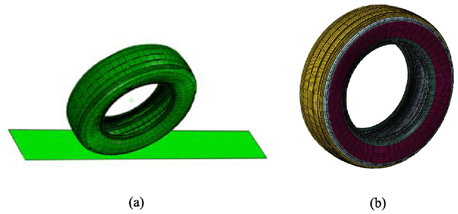
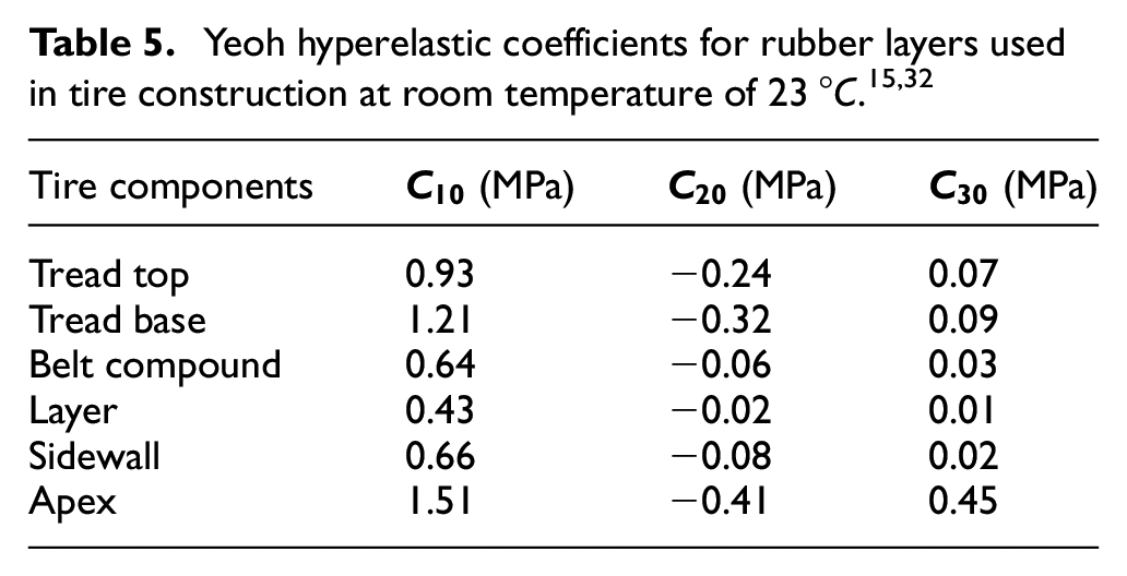
The layout of a passenger car radial tire precisely consists of 13 different sections including Tread top, Tread base, Cap ply, Ply, layers of Belts, Carcass, Inner liner, Wing, Sidewall, Beads, Apex, Anti-abrasion (abrasion gum strips). Figure 1 depicts the detailed geometry of a 185/65R14 tire. The structure and the mechanical properties of materials are stated in Table 1. The process of the investigation of the Poisson’s ratio and the coefficients of Yeoh hyperelastic model is stated in section 5 based on the previous published research.15,32
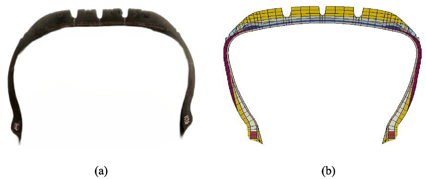
Tire-cross section: (a) A P185/65R14 88H PCR tire cross-section, (b) Tire full-axisymmetric FE model at unmounted rim state with different material properties.
Material properties of tire 185/65R14 H88. 15
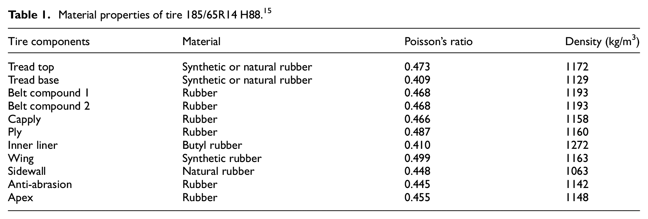
In this work, the reinforcement rebar layers are modeled as homogenous, isotropic, and linear elastic constitutive models. The mechanical properties of the reinforcement cords are stated in Table 2. The process of experimental testing used to calculate the mechanical properties of the reinforcement cords of tires are stated in section 5 based on the previous published research.15,32
Mechanical properties of the reinforcement cords.
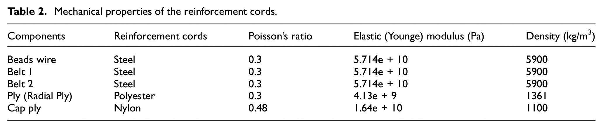
Rebar elements embedded in surface elements were used for the definition of steel cords of belts, Nylon cords of cap-plies, and Polyester cords of main body ply or carcass. 28 The carcass of the tire contains one body ply (polyester), two steel belts, and one nylon cap ply. 15 Using rebar elements for defining reinforcement cords considers the cord-rubber composite approach in the tire structure. 33 A small amount of skew symmetry is accrued due to the placement and various orientations of the reinforcing belts. 34 Tire reinforcement design parameters are stated in Table 3. The spacing for the cords are provided based on manufacturer catalog for this tire.
Rebar characteristics of reinforcing elements.
Development of finite element model and analysis procedures
To generate a finite element model of a 185/65R14 passenger car radial-belted tire commercial computer software Abaqus/CAE 35 was selected for pre-processing and processing tasks.
Axisymmetric
A full axisymmetric geometry of 184/65R14 88H passenger car radial tire was built in Abaqus /CAE. Abaqus /CAE is used as a pre-processor to generate input files for FE analysis. To complete the static analysis, the rubbery parts of the tire were meshed by 699 nodes, and the total 872 elements including Hybrid incompressible Continuum elements (CGAX4H) and the rebar layers of the tire such as cap-ply and belt reinforcement were modeled by Axisymmetric Surface elements (SFMGAX1) for the steady state rolling analysis. This model consists of belts and plies modeled with surface elements embedded in Continuum elements. 34 The rim mounting and inflation pressure analysis was performed with a 2D layout. To mount the tire on the rim, the beads were moved toward the center of the ring, 12.7 mm for each side in the lateral direction.
Arbitrary Eulerian/Lagrangian (ALE) and pure Lagrangian framework
To perform a steady state rolling simulation a restart command is deployed in the analysis which is carried out by the previous step results. Then, steady state rolling analysis restarts from a footprint analysis in which a mixed ALE (Arbitrary Eulerian/Lagrangian) framework has been adopted. Whereas in the transient simulation, the pure Lagrangian approach is implemented. ALE method includes, a moving refence frame in which the rotational movement of the rigid body is defined in the Eulerian coordinate and the deformation is defined in the Lagrangian frame. 26 The reference frame is connected to the rotating tire’s axle. Tire is not allowed to move in this frame, and it is fixed, however the material in tire’s structure can flow through the meshes which were generated in the tire’s finite element model. This method provides the capability of the modeling rolling tires by implementing pure Lagrangian formulation, because the reference frame which captures the motion is connected to the material. 26 The use of Eulerian and Lagrangian method at the same time, requires that the transitional movement of tire with linear longitudinal velocity, and the angular/spinning velocity will be defined independently from each other, and then these two velocities will be imported to the software as an initial inputs for the simulation. According to the equation (1), these two velocities are proportional.

Where r is the rotational radius and
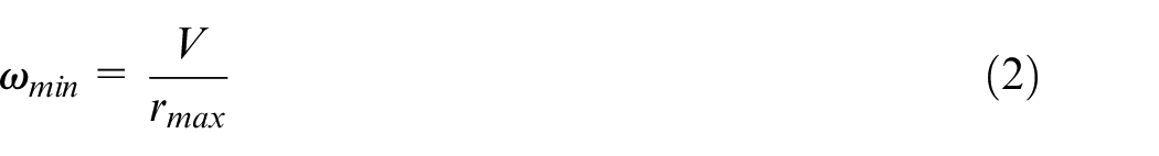
The tire has a curvature shape in the tread top pattern. As shown in Figure 2 during the tire-road interaction, the curvature in contact with the ground will be eliminated and then the rotational radius is not constant anymore. For this reason, in the presence of the longitudinal velocity of the tire, the corresponding angular velocity can be calculated. To solve this problem, firstly the linear velocity is assumed to be constant which has a value of 80 km/h. It must be noted that this specific velocity value has been chosen according to ISO 28580 to predict rolling resistance force. Secondly, the steady state rolling analysis is carried out for the specific range of the angular velocities varied between the minimum and the maximum value. These two angular velocities are calculated with equations (2) and (3), respectively.
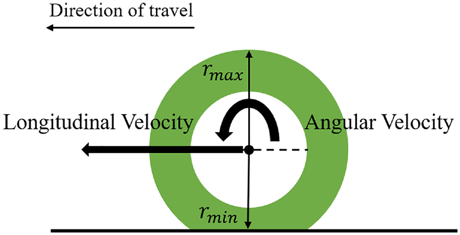
Side view of the rolling tire with the minimum and maximum rotating radius.
Where
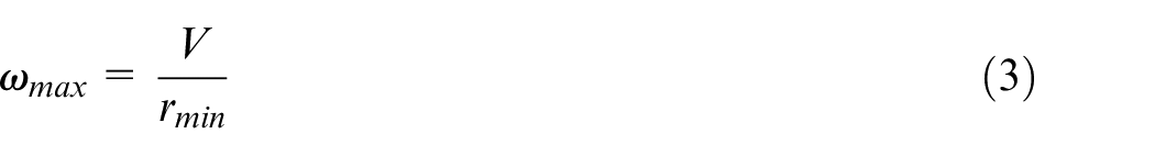
Figure 2 shows the minimum and the maximum radius of the tire in the steady state rolling condition.
3D static and steady state rolling
A corresponding 3D model was developed by using the capability of symmetric model generation in the Abaqus standard command line environment. The output results from 2D inflation pressure analysis were invoked as input data to start 3D static analysis using symmetric result transfer capability in Abaqus. For 3D static analysis a non-uniform discretization along the circumference of the tire was used, Figure 3(b). In this approach, the contact patch includes finer mesh, and the rest of the tire circumference was divided by coarse mesh. The tread pattern is modeled with three grooves as shown in Figures 1(b) and 3(a). The road is modeled by an analytical rigid surface. The full 3D tire-road model includes 47,687 nodes and 47,872 elements.
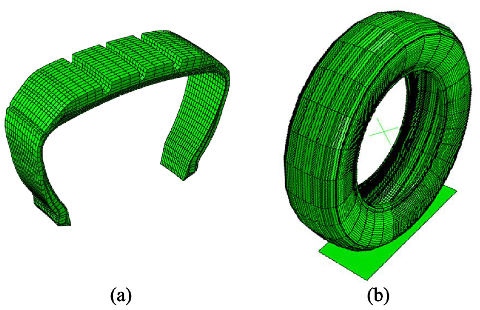
Tire 3D FEM model at implicit analysis: (a) Sweep section of the tire before the revolving command, and (b) three-dimensional finite element 184/65R14 88H tire model.
To model tire-road friction the Coulomb friction law was implemented according to Ghoreishy’s previous study.
28
To investigate the tire footprint, a normal concentrated radial (vertical) load was applied to the center of the rim via a rigid contact surface. To perform steady state rolling analysis, a built-in arbitrary ALE technique was implemented in Abaqus/Standard. In this method, linear and angular velocities must be specified independently. Therefore, a constant linear velocity of 80 km/h was considered, while the tire was subjected to rotational velocities that were varied between 65 and 85rad/s to perform the tire’s traction and braking simulations. To obtain steady state rolling motion, the steady state transport capability in Abaqus/Standard was implemented, and also an Abaqus subroutine was used to find free rolling solution
27
for tires traveling on a flat rigid surface. As a result, the angular velocity in which the longitudinal force (
Estimation of free rolling velocity for tire models.
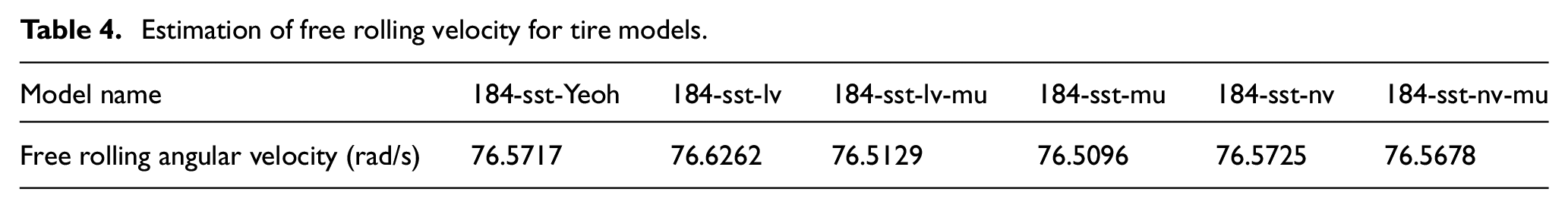
It should be noted that in this work various abbreviations were used to simplify and distinguish different models in all simulations such as 184-sst-lv-mu. For each FEM model of 185/65 R 14 tire, the number 18 reveals a symbol of the two first numbers of tire width, and the number 4 referred to the second number of ring size which is 14. Also, steady state rolling analysis is titled sst, and transient analysis using explicit solver is called xpl in this work. Besides, material definitions such as (a) linear viscoelastic referred to as Prony series, (b) non-linear viscoelastic referred to as PRF, and (c) Mullins Effect is addressed as, lv, nv, and mu respectively.
Transient dynamic analysis
To perform transient analysis, the continuation technique was used that fulfills some requirements: referred to as a kind of import rolling. For this purpose, the capability of transferring results between Abaqus/Standard and Abaqus/explicit was used during the analysis. The tire model for transient rolling differs slightly from that used in steady state transport. A configuration of the inflated tire model with deformed mesh and its associated material was imported to a new analysis in Abaqus/explicit for the subsequent transient dynamic analysis.34,36 The uniform discretization along the tire circumference was considered and then, the entire circumference of the tire was divided into 60 sections in the circumferential direction. Compared with standard analysis a finer mesh was used for tire geometry from the first step. The 2D tire model used for the explicit analysis was generated of 687 nodes and 854 elements including Continuum elements (CGAX4). As elements in explicit techniques must be compressible thereby tire was meshed by 59,854 reduced-integration axisymmetric continuum solid elements, Figure 4.
Explicit FE tire model: (a) Tire-road finite element model for explicit analysis (uniform discretization), (b) tire FE model material definition after revolving transport.
The total degrees of freedom of this 3D FE model amount to approximately 100,000. The wheel is modeled as a rigid steel body with a mass density of 7800 kg/m3. According to one of the standard procedures ISO 28580, the inflation pressure was set to 210 kPa and the vertical load of 4155 N corresponds to the axle weight applied to the tire in both static and transient analyses. Rim was modeled by rigid axisymmetric elements and rim nodes which interacted with the ring were fixed to the wheel using the tie technique and were modeled using Rigid elements in axisymmetric planar geometries (RAX2). The reference node of the road profile was modeled as a rigid body. In addition, a boundary condition of velocity type near the free-rolling velocity in the longitudinal direction was imposed on the center of the rim while all the other degrees of freedom were constrained to the ground. It allows the tire to rotate freely and move toward the longitudinal direction.
Material models (Definitions and experimental)
To model rubbery parts of the tire first the general concepts of rubber-based materials are reviewed. Then, the characteristics of compounding are studied using various experimental tests.
Hyperelastic
Rubbers present a highly non-linear elastic behavior under loading conditions 10 and also exhibit instantaneous elastic response up to large strains, 34 therefore small strain elasticity theory is not a useful method to describe rubber behavior. Another significant aspect of rubbers that distinguishes them from other materials is incompressibility, especially under compressive loads. Therefore, hyperelastic constitutive models that are in terms of strain energy function are used for the description of nonlinear stress-strain behavior in rubbery materials. Commercial FE software like Abaqus provides some of the hyperelastic constitutive models; such as Ogden, Arruda–Boyce, Polynomial and reduced Polynomial, Van der Waals, and Marlow that could be applicable over a wide range of strains. 37 Recent research has revealed that the type of hyperelastic equation has a significant effect on the precision of the results. 28 Therefore, the selection of a proper material model is an important factor. Among all the hyperelastic constitutive models, Yeoh had adequate accuracy and showed a reasonable curve fitting between numerical and experimental stress-strain test data, even at large values of strains. 38 The advantage of using the Yeoh model is its ability to simulate various modes of deformation with limited data access. 39 In this study, all the simulations are executed by implementing the Yeoh constitutive model for the mechanical property definition of rubber compounds. Yeoh hyperelastic model is an invariant-based model defined in terms of strain energy density with the following equation. 37
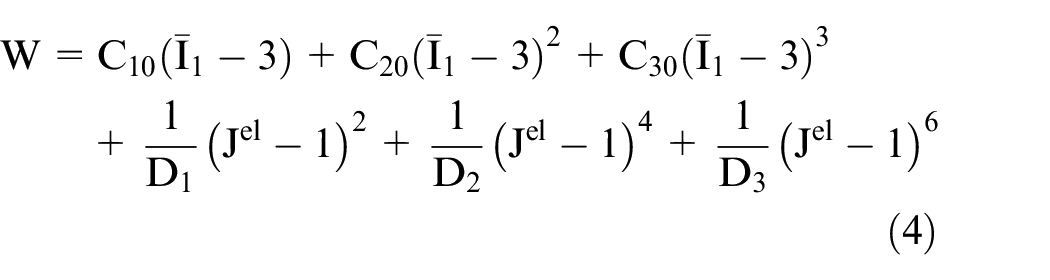
Where
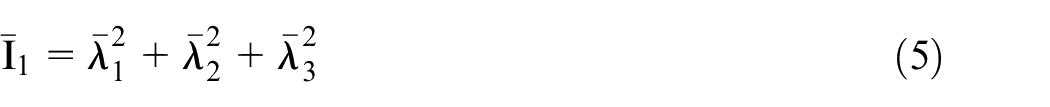
and
In the following equation
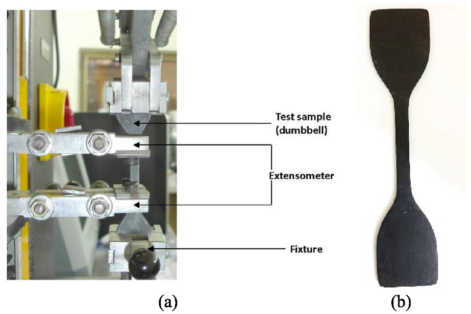
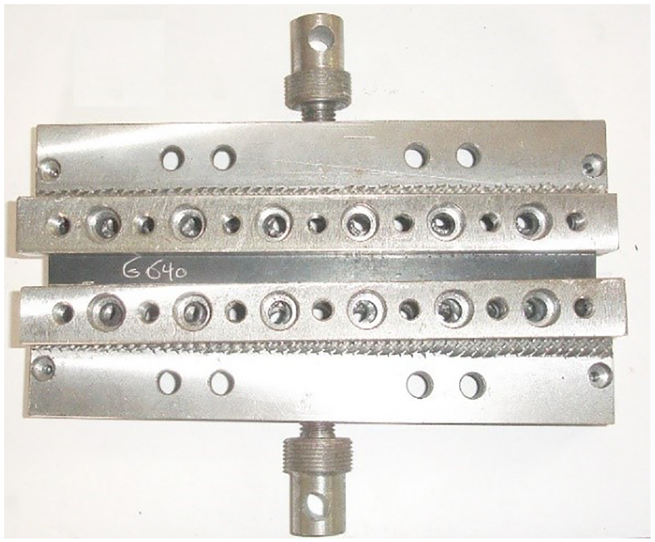
Experimental setup for the tensile test of a sample of tread compound: (a) Test setup with fixtures and extensometer used for uniaxial tensile test and (b) tensile test sample.
Furthermore, in addition to the tensile test, for measuring the hyperelastic behavior of the tire rubber compound, the compression with friction test was carried out according to ISO 7743 standard as shown in. This compression test was conducted by a universal testing machine to evaluate the compressibility of the compounds as shown in Figure 6.
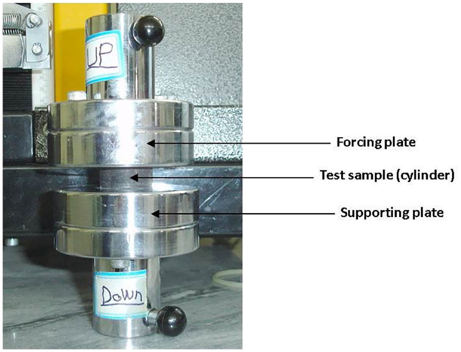
Rubber sample with supporting and forcing plates used for uniaxial compression test according to ISO 7743.
The tensile test for the compounds except the tread top and tread base was carried out at standard room temperature. To determine the coefficient of the Yeoh model, curve fitting based on the least squares method was implemented according to Ghoreishy’s previous work,15,32 and these results have been used in this work. Additionally, to determine the Poisson’s ratio of the rubber compounds a volumetric compression test also was performed as shown in Figure 7. The experimental results were then used to calculate the Poisson’s ratio based on the method described in the Ghoreishy. 40 The results of parameter identification for material model are given in the Tables 1 and 2.
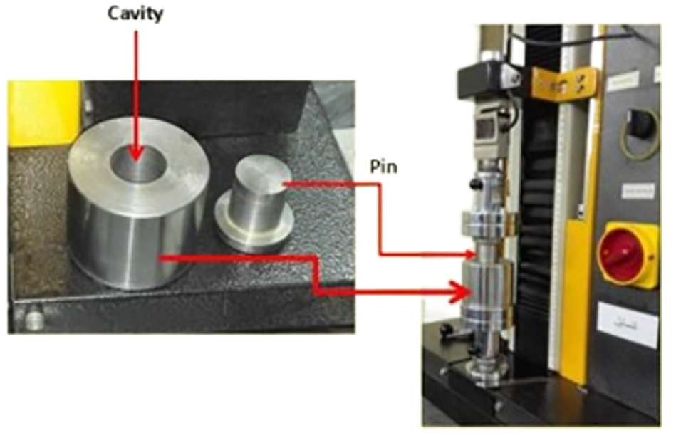
A volumetric compression test fixture (left) mounted in a universal test machine (right).
Moreover, a planar tensile test (pure shear) was conducted on the rubber compounds. During this test, a tensile load was imposed on a rubber strip as shown in Figure 8.
Rubber sample with fixture for the planar tensile (pure shear) test.
Yeoh constitutive equation material parameters are used in this research are implemented based on the previous published paper 15 and the coefficients are stated in Table 5.
Linear viscoelastic
Rubber compounds exhibit a linear variation of strain instead of applied stress undergoing tensile loads, 41 which is defined as linear viscoelastic behavior. In this situation energy is both dissipated and stored during deformation, known as the hysteresis effect. 42 It describes the viscous and elastic components of material behavior. In order to model the hyper-viscoelastic response, the expansion of the Prony series in conjunction with a hyperelastic equation is used.36,43 For the Yeoh model, the linear hyper-viscoelastic form of the constitutive equation could be explained as follows:
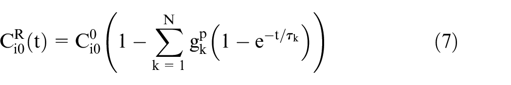
Where,
The relaxation parameters were determined by the author’s previously established method. 40 For this purpose, three rubber strips were cut from the cured sheet. The corresponding FE model of each strip was analyzed with a hyper-viscoelastic material model in Abaqus. Then, to determine the Prony series parameters, each model was optimized by implementing a non-gradient-based algorithm such as the Nelder–Mead method.
Nonlinear viscoelastic (Parallel rheological framework)
Nonlinear viscoelasticity describes a time-varying response (shear and volumetric behavior) to transient applications.36,42 This is a time-dependent behavior, in which stress relaxation or a decrease in storage modulus with an increase in amplitude known as the Payne effect, is manifested as a dependence on the time and the applied strain.15,44 To describe nonlinear viscoelasticity, creep, stress relaxation, or dynamic tests could be used. Dynamic Mechanical Analysis (DMA) is used to measure the response of rubber to an oscillatory deformation as a function of temperature. 45 In 2018, it was proved that stress relaxation test data are accurate enough for explaining the nonlinear viscoelasticity 46 in tire FE simulations, therefore the DMA was not implemented during viscoelastic material definition in this research. To determine the nonlinear viscoelastic behavior of rubber compounds, the PRF concept is implemented in this study. The parallel rheological framework defines the non-linear viscoelastic-elastoplastic model by a framework consisting of multiple viscoelastic networks and optionally an elastoplastic network connected in parallel as shown in Figure 9. One of the significant advantages of using a parallel rheological framework is the availability of this model to use with the Mullins effect. 34
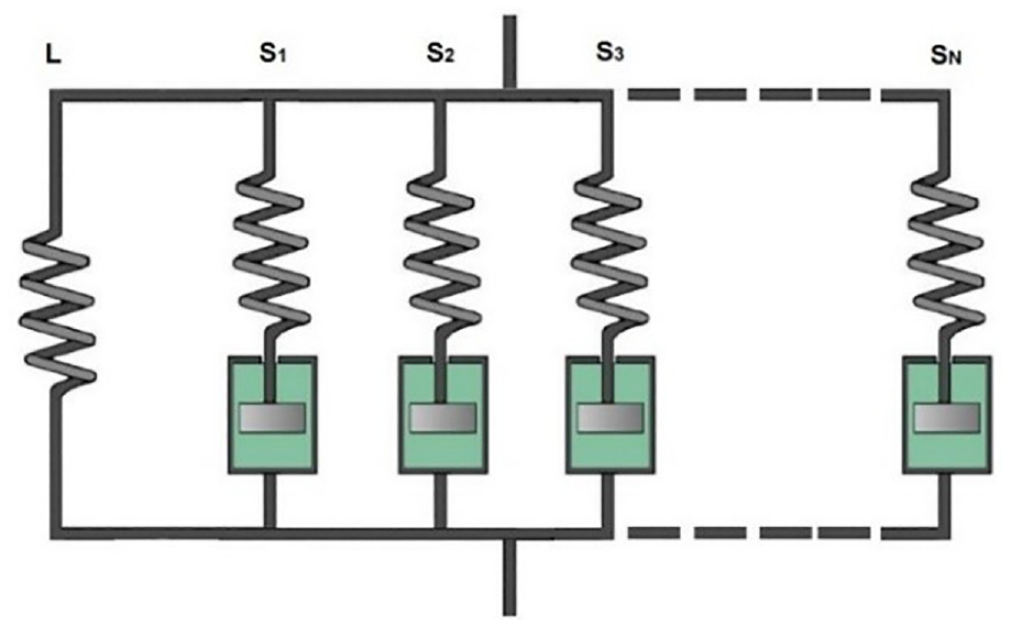
Schematic of the nonlinear viscoelastic model with multiple parallel networks.
In this study, the Yeoh constitutive model is used to describe the elastic response in a parallel rheological framework therefore, the total strain energy function is expressed as below.
Where
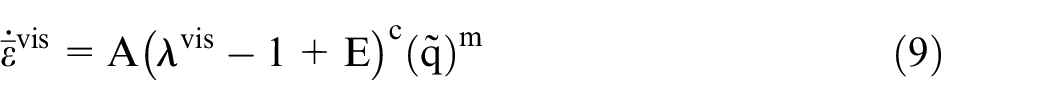
The Bergstrom-Boyce creep law is specified by providing four parameters, where E, c, A, and m are material parameters.
Stress softening effect (Mullins effect)
The Mullins effect is a phenomenon that very often occurs in highly filled rubber compounds, (especially those which are used in tires), due to cyclic loading conditions 6 as shown in Figure 10. The Mullins stress softening can be considered a damaging phenomenon that only depends on the maximum stretch attained during the deformation history. 48 Such progressive damage usually occurs in the first few cycles and the material response will soon achieve an ideal stable state after tracing a few loading-unloading cycles. 49 In this case, rubber leaves abrasion and damage thereby it would bring residual strain and anisotropy which have an important effect on tire rolling resistance.
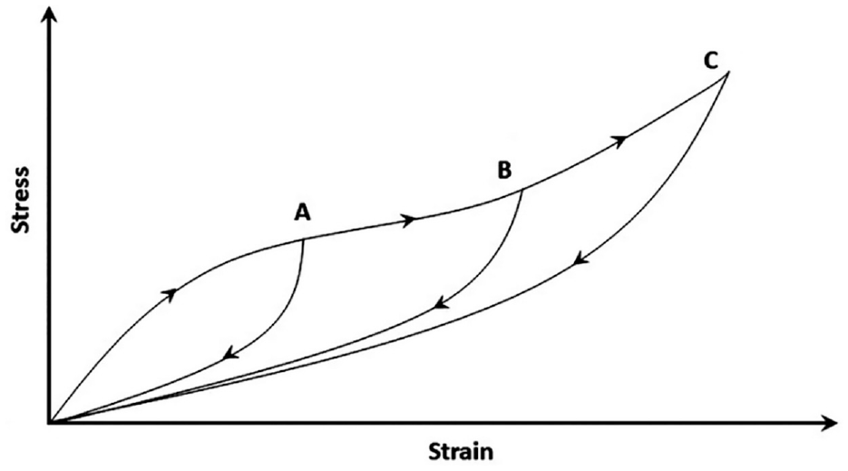
Typical behavior of filled elastomers under cyclic loading conditions.
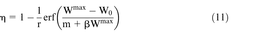
In this sense, the material response could be governed by the strain-energy function on unloading and subsequent loading as follows 50 :

Where W (F, η) is the new strain energy function,
Where
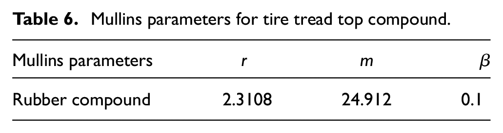
Mullins parameters for tire tread top compound.
Results and discussion
Two sets of several analyses consisting of two types of solver and various material definitions were carried out in this study and the rolling resistance and the tire footprint were extracted. The results are presented in the next sections.
Rolling resistance force at steady state rolling
The first series of analyses were carried out using Abaqus/Standard to find the effect of various adopted material models on rolling resistance. Tire reaction force from the road reference point was extracted from steady state rolling analysis as shown in Figure 11. To predict rolling resistance force in steady state rolling method, firstly the problem is solved without considering (regardless of) dissipative parameters such as Viscoelasticity and Mullins effect (model 184-sst which includes only Yeoh hyperelastic definition). And then the angular velocity in which the value of longitudinal force is equal to zero, will be calculated using the subroutine program. This angular velocity called free rolling angular velocity or (angular velocity at free rolling
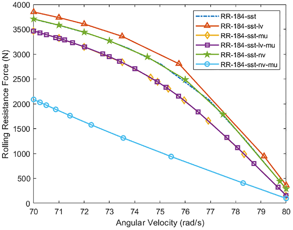
Tire rolling resistance force versus angular (spinning) velocity for a constant linear velocity of 80 km/h in the steady state rolling analysis.
Secondly, in the next step, dissipative parameters such as Viscoelasticity and Mullins effect will be added to the problem, and then the value of the longitudinal force is calculated at the angular velocity in which free rolling was occurred (previous step). The value of the calculated force is not zero because the dissipative factors have been added to the problem. The difference between the calculated force and the reaction force (which was captured in the model 184-sst) in the absence of dissipative parameters, results in a non-zero value. This value is called rolling resistance force. Furthermore, it should be mentioned that the steady state rolling method, the linear velocity and angular velocity are independently defined as inputs for the problem, while it is obvious that these two parameters are not independent from each other. It must be noted that basically, the rolling resistance force is increased by increasing the linear velocity. 10 However, Figure 11 shows the variation of rolling resistance force versus angular velocity (not linear longitudinal/ground velocity).
As shown in Figure 11, with an increase in the angular velocity at constant linear velocity, a traction in the forward direction is generated. Therefore, a portion of the force required for motion, is provided through traction in the forward direction, and then this leads to a decrease in the rolling resistance force. In addition, similarly, in the opposite case when angular velocity decreases, as the tire is heading toward braking, therefore resistance to motion increases and the value of rolling resistance force will be increased. In other words, what is considered as rolling resistance is actually the summation of the rolling resistance force and the additional (residual) force that moves the tire toward traction or braking.
It should be pointed out that linear velocity has a constant value of 80 km/h for steady state rolling analysis. As in this simulation, the steady state rolling method is implemented, the linear velocity is kept constant, and the angular velocity varies from the lower values (70 rad/s) to the higher value (80 rad/s) which correspond to the braking and the traction, respectively.
In Figure 11, the rolling resistance force of the 184-sst-lv model, decreased to the minimum level in which the Prony series was implemented. Since the calculations were carried out during the fully relaxed condition for the tread rubber compound, the time-dependent properties were ignored. By contrast, the rolling resistance force in the 184-sst-nv-mu model decreased dramatically to the minimum value. Negligible differences were found between the 184-sst-Yeoh and 184-sst-nv models and these models differed slightly from each other at the higher angular velocities between 74 and 77 rad/s. Rolling resistance force in the 184-sst-mu model and in the 184-sst-lv-mu model almost has the same trend. This result also reveals that by increasing the spinning (rotational or angular) velocity in the steady state rolling at the 80km/h linear velocity, rolling resistance force will be decreased. Therefore, by exiting the hyperelastic zone, the rubber behavior is not linear anymore. As shown in Figure 11, the elastic response of tire compounds in the model 184-sst-Yeoh including Yeoh hyperelastic material model is considered as an original reference trendline. While adding the different effect, all the other models will be compared to this model to determine the energy dissipated for each model. The deducted force of each model from the force in the pure hyperelastic model, 184-sst-Yeoh is considered as rolling resistance force.27,51 The advantage of this method is that with the less computation time, the tire behavior in dynamic conditions can be predicted.
Experimental validation
The rolling resistance force is defined in the opposite direction of the longitudinal force (
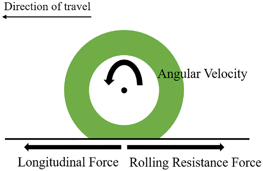
Schematic view of rolling resistance force and longitudinal force.
Moreover, Rolling Resistance Coefficient (RRC) can be calculated based on the following equation. 10
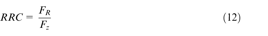
Where
Tire footprint in the steady state and transient conditions
Tire footprint analysis was obtained using two different methods, the arbitrarily mixed Lagrangian-Eulerian and the pure Lagrangian approach carried out using the implicit and explicit solver, respectively. During this work, it was investigated that the implicit solver of Abaqus had some drawbacks to calculate nonlinear viscoelasticity in conjunction with the Mullins effect, on the contrary, the Abaqus/Explicit was capable to model the combination of different hyper-viscoelastic models and Mullins effect for tire simulation purposes. On the other hand, to facilitate the convergence issues, a do-nothing step was performed during the steady state transport analysis that was carried out by applying the damage response through the Mullins effect ramped on gradually over the step. As expected, the results of repetitive analyses confirmed that the damage associated with the Mullins effect is independent of the angular velocity. 36 Particularly, Mullin’s effect convergence issues resulted in the use of Abaqus/Explicit instead of the implicit solver to accomplish the effect of material models. The time of total dynamic transient simulation is taken 0.82 s for one full tire revolution in straight rolling. The maximum contact pressure distribution was obtained for both static and transient dynamic analyses; the results are shown in Figures 14 and 15. For instance, Figure 13 shows the tire contact pressure distribution for the static footprint which is obtained during the steady state rolling analysis. The result shown in Figure 13 is the contact patch contour for the 184-sst-lv simulation, in which the combination of two material models including hyperplastic (Yeoh) and linear viscoelastic (Prony) is implemented. Generally, it can be noted that since the tread surface particularly the upper tread (tread top), has curvature in its shape when the tire undergoes with interaction with the road, curvatures in the tread pattern in contact with the road, will be eliminated. Consequently, the tire shoulder and the tire sidewall experienced more pressure as shown in red color in the contour. 51
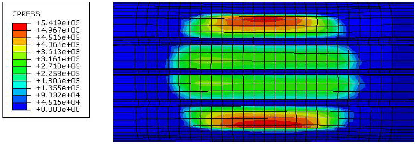
Contact pressure distribution at the contact-patch region in the static footprint for the combination of Yeoh hyperleastic model and Prony series (184-sst-lv model) with 4155 N vertical load and 210 kPa inflation pressure.
As shown in Figure 14 among static footprint results, the model named 184-sst-lv with linear hyper-viscoelastic material definition resulted in the maximum contact pressure distribution in the footprint area. Moreover, contact pressure distribution remained relatively stable at the minimum values for the 184-sst-mu and 184-sst-lv-mu models.
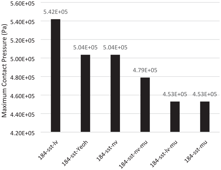
Maximum tire contact pressure in the steady state rolling analysis.
On the other hand, as shown in Figure 15 among explicit analyses, the footprint at the 184-xpl-mu rose dramatically to a peak of 9.374E + 06 Pa by applying the Mullins effect in transient conditions. However, the Mullins effect in steady state rolling analysis in the 184-sst-mu model provided a negligible amount of tire footprint. By contrast, the 184-xpl model consisting of the hyperelastic model has a minimum contact pressure because of neglecting the non-linear viscous behavior of the rubber. In addition, contact pressure in 184-xpl-nv-mu, including PRF and Mullins effect, increased significantly due to time-domain formulation in material computation. It is observed that using the Mullins effect generally predicts higher contact pressure values, which is an indication of better material history and time-dependent property representation.
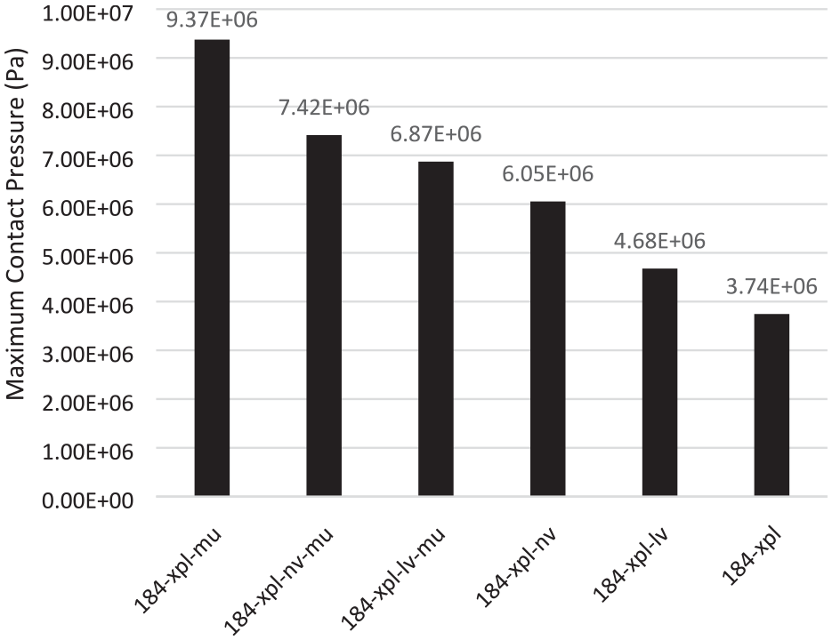
Maximum tire contact pressure in the transient analysis.
Another significant factor in contact pressure distribution that differs between static and transient analyses was the asymmetry of contact pressure distribution between the front and rear tire footprint in explicit simulations.27,51 It is mainly due to viscoelasticity and relaxation time. Since the material behavior is a function of time, therefore in each point of the tread compound (front and rear zone of the contact patch), there is a different material history. While tire rolls over the ground, the front points of the compound in the tread which enter the contact zone is not fully relaxed. Consequently, the material behavior in the front zone of the contact area is completely different from the points which are located in the rear zone of the tire contact patch. Moreover, as the tire tread is built from various compounding, it means that each point of the tread compound is simulated with different material characteristic during the finite element analysis. Since material behavior is the function of time, when the tire enters the contact region, it takes a period of time to pass through the contact zone then it enters the footprint zone. Besides, the tire revolution is periodic, and each cycle takes time. For this reason, cyclic revolution does not allow the material to relax completely and reach its final state. Therefore, the time difference directly effects the tire behavior due to material history phenomena. This leads to obtain different results in the contact pressure contour, as well.
In other words, when the viscoelasticity is not considered in the analysis, the simulation is carried out based on the fully relaxed material and as a result the model 184-sst-mu shows the minimum contact pressure distribution. On the other hand, while viscoelastic properties of tire compounds are added to the problem, the model 184-sst-lv reveals the maximum contact pressure because the material is not in completely relaxed when the viscoelasticity is included. Moreover, the contour is not symmetric anymore. Tire footprint experiences a non-symmetric (asymmetric) contact pressure distribution field. 51
This was also induced by the time-dependent material stiffness. It should be noted that the asymmetric tire contact pressure distribution in footprint analysis was relative to the relaxation time of tire rubber compounds particularly, tread top and tread base compounds. 27
As observed in Figure 15, the material viscosity in the tread top and tread base compounds have a significant effect on the footprint analysis. Additionally, the stiffness of tread rubber compound constantly changes over time, this leads to emerging asymmetry in contact pressure distribution in the transient dynamic rolling.
Wheel reaction force in the transient dynamic rolling tire
Wheel-rim reaction force was predicted using the road reference point because the suspension system was not modeled in this study. The road reaction force reveals some numerical noise. To remove high-frequency numerical noise in the transient results, the tire center reaction force was filtered using the SAE60 filter as shown in Figure 16 in the post-processing analysis. Additionally, Abaqus/CAE refers to the value of 100 to determine the cut-off frequency multiplier (CM) for the SAE60 class filter operators. 36 Since the transient rolling analysis was generated using an import steady state transport method from previous time steps (0–5 s) in the previous analyses, then the rim reaction force was extracted over a period of 5–6 s at straight traveling with a cleat.
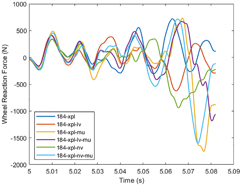
Vertical reaction force magnitude at the wheel reference point filtered by SAE 60 filter.
According to Figure 17, the 184-xpl-lv-mu model, has the lowest wheel reaction force which reveals the effect of linear viscoelasticity with material convection calculations in a fully relaxed long-term solution. Besides, considering stress softening effect of the tire compounds in the 184-xpl-lv-mu model, it shows that adding the Mullins effect leads to a lower wheel reaction force and the displacement of the axle center in this model is at the lowest value. On the other hand, the combination of the PRF model and the Yeoh hyperelastic model results in the maximum wheel reaction force due to the exhibition of the permanent set in the non-linear viscous behavior of the tire rubber.
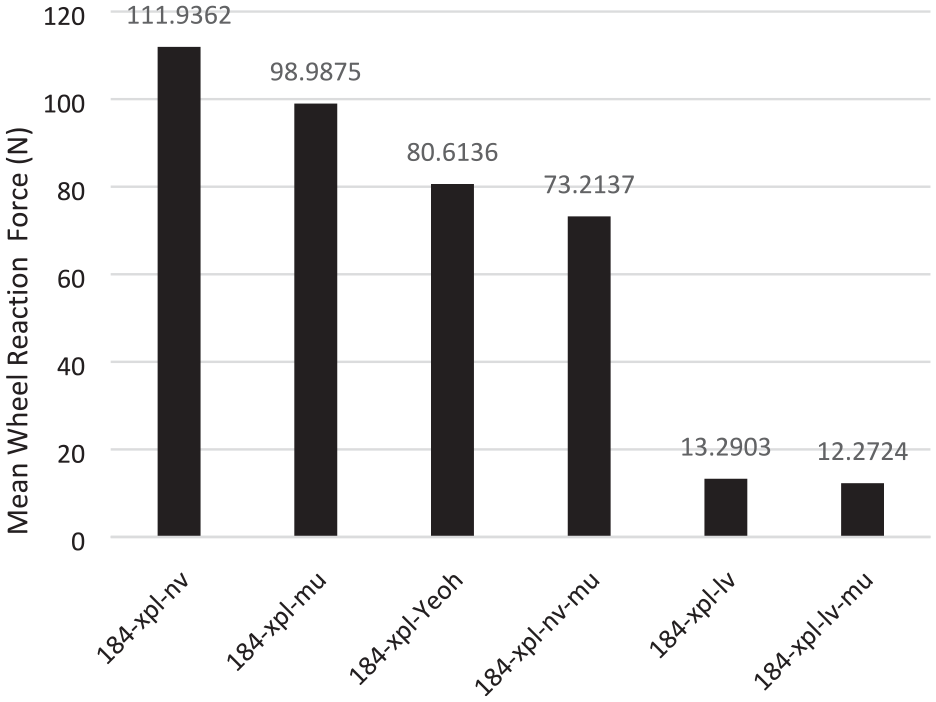
Mean vertical reaction force magnitude at the wheel reference point.
Conclusions
The rolling resistance in a 184/65R14 88 H passenger car tire was predicted via FEA. The rolling resistance was calculated by adopting the linear viscoelastic and nonlinear-viscoelastic models, particularly considering the Mullins effect. Additionally, it was clarified that the rolling resistance force is very sensitive to the implemented viscoelastic model combined with the Mullins effect. The PRF nonlinear viscoelastic model with the Mullins effect could predict the rolling resistance force more accurately because material definition entails energy dissipation over time. Moreover, a comparison of the obtained results from steady state rolling and transient dynamic analysis indicated that the adopted hyper-viscoelastic model has a significant impact on the contact pressure distribution of the tire contact patch. The Mullins effect increases the contact pressure dramatically in transient dynamic analysis. Additionally, implementing the non-linear viscoelasticity with the Mullins effect results in increasing the contact pressure distribution at transient dynamic analysis. It should be noted that the type of the material model is a critical selection for the convergence issue. Also, for the pure Lagrangian method a finer mesh results in a good conversion with the implemented material model. The wheel reaction force also was very sensitive to the adopted parallel rheological framework model.
Footnotes
Correction (June 2024):
Article updated to correct Figures 2 and 12.
Declaration of conflicting interests
The author(s) declared no potential conflicts of interest with respect to the research, authorship, and/or publication of this article.
Funding
The author(s) received no financial support for the research, authorship, and/or publication of this article.