Sage Journals: Discover world-class research

Abstract

Instantaneous fuel consumption estimation of fleet vehicles provides essential tools for fleet operation optimization and intelligent fleet management. This study aims to develop practical and accurate models to estimate instantaneous fuel consumption based on on-board diagnostics (OBD) data. Fuel consumption data is measured by a high-precision fuel flow meter. Two machine learning algorithms of Random Forest (RF) and Artificial Neural Networks (ANN) are trained with real-world urban and highway driving data of four fleet vehicles with different types and powertrain systems. In addition, the cold-start period of the vehicle operation is included to cover the fuel consumption penalty in the warm-up period. The validation results show that the RF method is more accurate than the ANN method, and both of the machine learning models have a better accuracy compared to the existing fuel consumption calculation methods based on the engine control unit (ECU) parameters.

Keywords

Instantaneous fuel consumption machine learning intelligent fleet management random forest artificial neural networks real-world driving data

Introduction

Intelligent fleet management systems aim to improve efficiency and reduce costs of operating fleet vehicles, while complying the fleet operation with regulations and environmental responsibilities.¹ Fuel consumption is one of the major operating expenses in a fleet which has a direct impact on the emission of greenhouse gases and air pollutants from fleet vehicles. Therefore, monitoring the fuel consumption of fleet vehicles is one of the important tasks involved in fleet management.^2,3

There exist methods for calculating “average” fuel consumption based on the total amount of fuel consumption and the distance traveled.⁴ However, for fleet management systems to minimize fuel consumption, cumulative or average fuel consumption is often insufficient as the average data does not provide enough information to:

detect driving situations that result in high fuel consumption and CO₂ tailpipe emissions^5,6

determine powertrain efficiency under various operating circumstances

choose the optimal (i.e. fuel-efficient) routes⁷

determine how fleet driver behavior affects fuel consumption^8,9

develop fuel-specific emission factors in different driving conditions¹⁰

perform dynamic optimization and control^11,12

As a result, “instantaneous” fuel consumption monitoring offers additional benefits for intelligent fleet management systems compared to average fuel consumption.¹³ Given fleet vehicles are commonly equipped with global positioning system (GPS), instantaneous fuel consumption, along with vehicle location and road grade data, can be utilized to understand the total fuel consumption of individual vehicles and then used to develop intelligent fleet management strategies for route selection, vehicle type selection, and driver training.

Engine operational parameters and fuel consumption are correlated. Many engine performance parameters are accessible through on-board diagnostics (OBD) from the electronic control unit (ECU) of the vehicle. These parameters demonstrate real-time engine operation and have been used extensively in fleet management applications.^14,15 Some parameters provided by OBD affect fuel consumption, so these parameters can be used to estimate a vehicle instantaneous fuel consumption.

Instantaneous fuel consumption can be obtained through the three following methods:

ECU torque-based estimation: For some vehicles, an estimation of instantaneous fuel consumption is provided through the OBD data from the engine ECU. This could be based on the estimated engine torque and the steady-state brake specific fuel consumption (BSFC) map. These estimations are inaccurate under engine transient operation which is common for on-road vehicles.^16,17

ECU air-fuel-ratio-based estimation: Fuel consumption can be estimated by the intake air mass flow rate (MAF) and the air to fuel ratio commanded by ECU.¹⁸ This method also has limitations and can be inaccurate. For example, the ECU-commanded air-fuel equivalence ratio is not necessarily equal to real air-fuel equivalence ratio. In addition, the MAF data is not available from OBD data in all vehicles.¹⁹

Direct measurement: By installing a fuel flow rate sensor in the engine fuel feed line, instantaneous fuel consumption can be measured. This method requires a dedicated data collection system, an expensive sensor, and costly system maintenance.²⁰ Besides, a vehicle with a compression ignition (diesel) engine requires two fuel flow meters in the supply and return fuel lines.

An alternative method is to develop data-driven mathematical models based on available engine parameters through OBD data and measured fuel consumption for training the models. In this approach, OBD and measured fuel consumption data from representative fleet vehicles are collected to create models. Once experimentally validated models are developed, the instantaneous fuel consumption of the fleet vehicles is estimated from the OBD data of each vehicle. Machine learning methods are useful to develop data-driven models based on measured data.²¹

The approach used in this paper to estimate the instantaneous fuel consumption of fleet vehicles is implemented as a case study on the transportation fleet of the University of Alberta. The fleet of the University of Alberta consists of 173 vehicles, all of which are tracked daily utilizing cellular GPS and telematics OBD readers as part of an intelligent fleet management system. This study aims to develop a reliable and accurate machine-learning-based method for monitoring the instantaneous fuel consumption of university fleet vehicles using OBD data. Four different vehicles are chosen as representatives of the fleet to collect data in two different real-driving scenarios – highway driving and urban driving. This study includes extensive data collection at 2 Hz sampling frequency for four fleet vehicles.

The University of Alberta is located in Edmonton, which is a city with a cold climate and long winters, therefore the cold start period of vehicle engines is long and the fuel consumption penalty during the cold start period is high.²² In the urban driving scenario, which is shorter, the cold start period is more significant. In this study, the cold start interval is covered so that the fuel consumption penalty in the cold start is also included in the models.

Machine learning algorithms have recently been used to estimate vehicular fuel consumption, both at the vehicle level and at the fleet level.²³ One of the ways to categorize different studies in this field is to divide the models into average and instantaneous fuel consumption models.

Wu and Liu^24,25 developed back-propagation and radial basis artificial neural networks (ANN) models to predict the average fuel consumption of vehicles during Environmental Protection Agency (EPA) Federal Test Procedure or FTP-75 driving cycle. The model inputs include vehicle make, vehicle weight, engine style, and transmission type. Radial basis ANN performed better compared to back-propagation ANN models. Zeng et al.²⁶ used a large-scale dataset to develop machine learning models to predict average fuel consumption based on multiple vehicle and trip variables (e.g. trip distance, average speed, number of intersections per km, engine displacement volume, and the coefficient of variance of speed). Among the algorithms utilized, support vector machines (SVM) model offered the best prediction compared to the multiple linear regression model and ANN. In another study, Gong et al.²⁷ compared different machine learning algorithms on a large data set of 1153 trips from 34 heavy-duty diesel trucks to predict average fuel consumption. Different categories of influencing factors were considered including vehicle-related factors (e.g. engine and transmission operating state), environment-related factors (e.g. weather condition), driving-related factors (e.g. driver behavior), and road-related factors (e.g. road grade). The random forest (RF) method showed the best prediction performance of all algorithms tested.

Katreddi and Thiruvengadam²⁸ estimated instantaneous fuel consumption based on very few key parameters including engine load, engine speed, and vehicle speed, using different machine learning algorithms. All data, including fuel combustion rate, was collected through OBD port of ECU. The study shows that ANN performed slightly better than other machine learning techniques such as linear regression and RF. Moradi and Miranda-Moreno¹⁸ used support vector regression (SVR) and ANN machine learning methods to develop vehicle-specific instantaneous fuel consumption models based on GPS and inertial measurement unit (IMU) data, accessible through smartphones. To improve the estimation accuracy, they trained a separate model to estimate engine speed based on the available GPS and IMU data and used it as a feature for the final model of each vehicle. The fuel consumption data used to train the models is an estimated fuel consumption based on OBD data. Another study by Kanarachos et al.²⁹ used smartphone’s GPS parameters to estimate instantaneous fuel consumption by different ANN models. They also used the OBD-calculated fuel consumption to train the models. They concluded recurrent ANN models are more appropriate compared to long-short-term-memory combined with ANN models to estimate fuel consumption. In a study by Vilaça et al.,³⁰ different machine learning models are compared and a boosted trees algorithm provided the most accurate estimate of fuel consumption based on GPS-derived speed, acceleration, and road grade. Perrotta et al.³¹ used three algorithms of SVM, RF, and ANN to estimate instantaneous fuel consumption of a large fleet of trucks based on truck telematics, road geometry, and condition data. RF was the most accurate model for estimation. In a study by Wickramanayake and Bandara,³² instantaneous and cumulative fuel consumption of a bus over a specific route was modeled using different machine learning models based on GPS data. Fuel consumption data was collected using a capacitive fuel sensor. Based on the analysis, it can be concluded that the RF technique produces a more accurate prediction compared to other utilized techniques, including gradient boosting and neural networks.

The majority^{18,28,29,33–36} of previous studies to model instantaneous fuel consumption of vehicles used ECU-estimated fuel consumption. However, ECU estimation is inaccurate particularly under transient conditions.³⁷ In addition, many studies did not consider cold start and non-stoichiometric operating conditions of the vehicles.^{13,18,24,26,29,33,35,36,38} Furthermore, some of the prior studies need GPS data for accurate instantaneous fuel consumption estimation.^{13,18,29,32,33,35} This study aims to address the existing gap in the literature by presenting a practical and accurate instantaneous fuel consumption estimation method that: (i) only requires OBD data, (ii) is based on actual fuel consumption measurement data, (iii) includes cold start and warm-up periods of vehicles, and (iv) is experimentally validated for different vehicle types (sedan, SUV, pickup truck), and different powertrain types (conventional internal combustion engine, hybrid electric, plug-in hybrid electric) for engines ranging from 1.5 to 6.2 l. This study applies an ultrasonic fuel flow meter which allows to measure ultra low-volume fuel flow operation with a sampling frequency as high as 5 Hz. Using fuel consumption and OBD data, accurate machine learning fuel consumption models are developed for both urban and highway driving conditions.

Methodology

Driving routes

Two different driving routes were selected for two different driving cycles of highway and urban driving. Both routes are designated to cover broad ranges of driving conditions. The highway route is longer and mostly consists of highways and out of town roads, while the urban route goes through urban streets and avenues. The origin and destination of both routes are the University service station located at the University of Alberta South Campus.

Highway driving route

The highway route, shown in Figure 1(a), starts in residential and urban areas but highway driving is the dominant part of it. The total distance of the route is 100 km with a duration of about 1 h and 30 min. The ratio of highway driving condition to the total distance covered is 75%.

Figure 1.

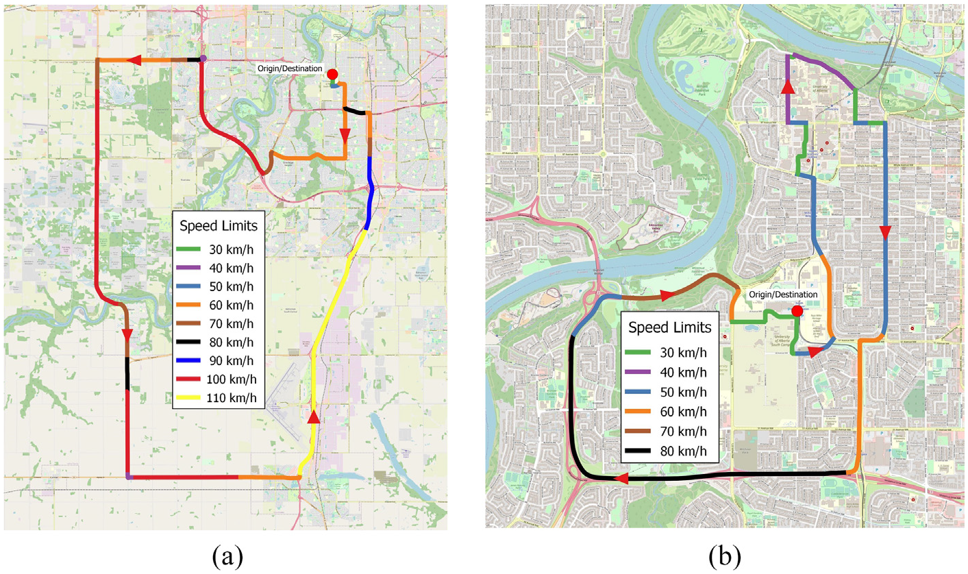
Test routes used in this study in Edmonton and suburbs: (a) the 100 km highway driving route and (b) the 20 km urban driving route.

Urban driving route

The urban route, shown in Figure 1(b), mostly covers residential and urban areas and includes 31 intersections with traffic lights, 13 intersections with stop signs, and six pedestrian crossing lights. It passes through the University of Alberta North Campus, the campus with the highest population and the site of the majority of the university-related activities. The speed limit in the campus part of the driving route ranges from 10 to 40 km/h. The total distance is 20.5 km long and takes roughly 36 min to complete. Urban driving conditions account for 70% of the entire distance traveled.

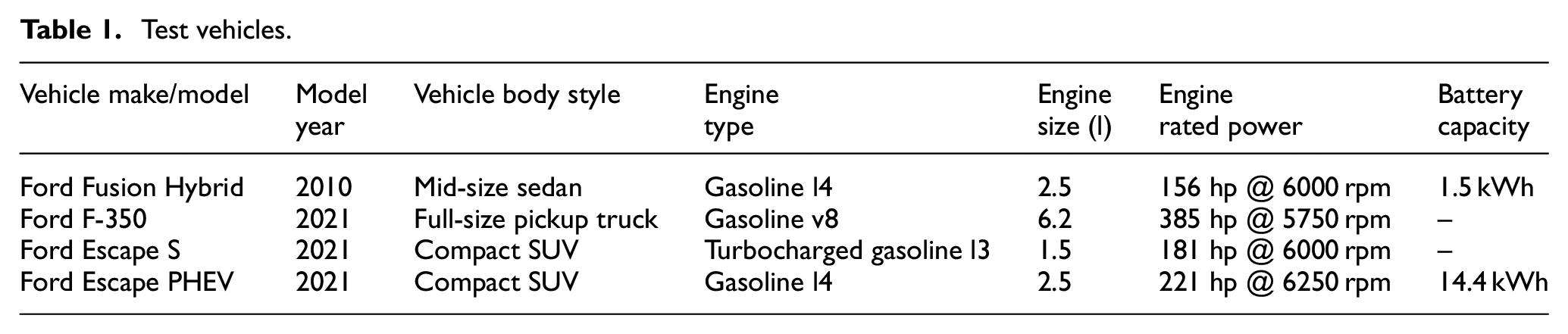
Test vehicles

The four vehicles selected for this study are listed in Table 1. The vehicles include a hybrid electric sedan, a full-size pickup truck, a conventional compact sports utility vehicle (SUV), and a plug-in hybrid electric (PHEV) SUV. These vehicles are a good representation of the main vehicle types of the University of Alberta fleet. Table 1 shows the selected vehicles specifications. These vehicles have distinct powertrain systems, including 2.5-l hybrid electric, 2.5-l plug-in hybrid electric, 1.5 l turbocharged, and 6.2-l gasoline engines.

Table 1.

Test vehicles.

Vehicle make/model	Model year	Vehicle body style	Engine type	Engine size (l)	Engine rated power	Battery capacity
Ford Fusion Hybrid	2010	Mid-size sedan	Gasoline l4	2.5	156 hp @ 6000 rpm	1.5 kWh
Ford F-350	2021	Full-size pickup truck	Gasoline v8	6.2	385 hp @ 5750 rpm	–
Ford Escape S	2021	Compact SUV	Turbocharged gasoline l3	1.5	181 hp @ 6000 rpm	–
Ford Escape PHEV	2021	Compact SUV	Gasoline l4	2.5	221 hp @ 6250 rpm	14.4 kWh

Fuel flow measurement

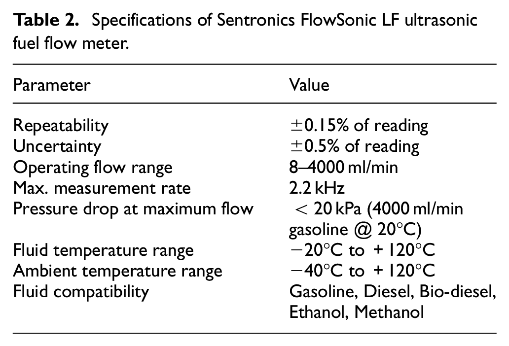
An ultrasonic fuel flow meter was installed on each vehicle to measure instantaneous fuel consumption, as shown in Figure 2. The fuel flow meter was Sentronics FlowSonic^® Low-Flow Sensor with the technical specifications listed in Table 2. This fuel flow meter was chosen for its ability to measure low-volume fuel flow (as in the idling condition of a small fleet vehicle), its capability to measure various fuels (e.g. gasoline and diesel), its robustness against vibrations and pulsating flows, its high measurement accuracy, and its small size and light weight that make it simple to install on any engine. Using a sampling rate of 5 Hz, the fuel flow data were recorded and sent to the data acquisition system through a controller area network (CAN) connection.

Figure 2.

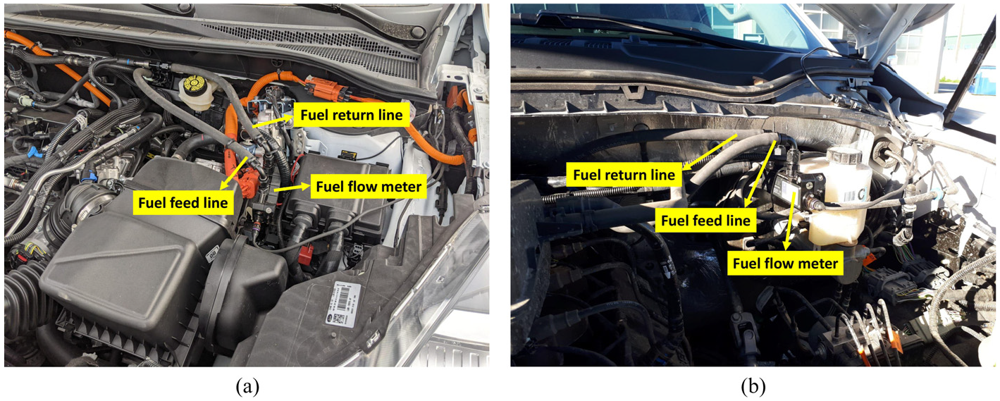
Fuel flow meter installation in the fuel path of the studied vehicles: (a) Ford Escape PHEV and (b) Ford F-350.

Table 2.

Specifications of Sentronics FlowSonic LF ultrasonic fuel flow meter.

Parameter	Value
Repeatability	±0.15% of reading
Uncertainty	±0.5% of reading
Operating flow range	8–4000 ml/min
Max. measurement rate	2.2 kHz
Pressure drop at maximum flow	<20 kPa (4000 ml/min gasoline @ 20°C)
Fluid temperature range	−20°C to +120°C
Ambient temperature range	−40°C to +120°C
Fluid compatibility	Gasoline, Diesel, Bio-diesel, Ethanol, Methanol

CAN data collection

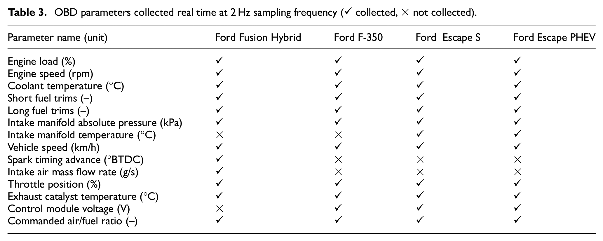
The data collection procedure utilizing a CAN data logger is shown in Figure 3. OBD data was collected over the CAN bus and synchronized with Sentronics sensor fuel measurement data. CAN data, including OBD and fuel flow measurement data, were collected using the CSS Electronics CANedge2 CAN data logger. The CAN data logger recorded OBD data at a sampling rate of 2 Hz and synchronized it with fuel flow CAN data. Table 3 shows the OBD parameters that were collected by the CAN data logger (CANedge2) for each tested vehicle.

Figure 3.

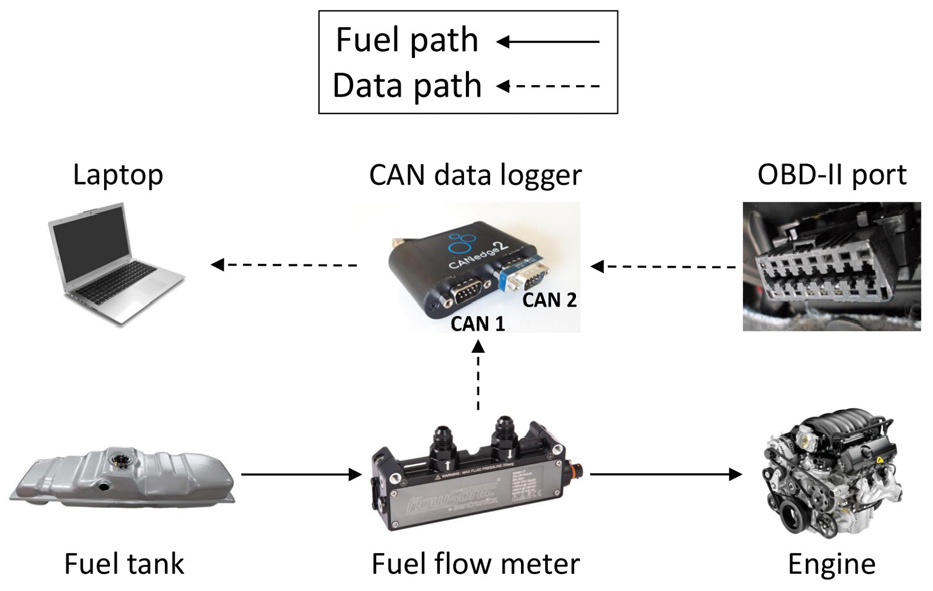
Schematics of the data collection process using CAN.

Table 3.

OBD parameters collected real time at 2 Hz sampling frequency (✓ collected, × not collected).

Parameter name (unit)	Ford Fusion Hybrid	Ford F-350	Ford Escape S	Ford Escape PHEV
Engine load (%)	✓	✓	✓	✓
Engine speed (rpm)	✓	✓	✓	✓
Coolant temperature (°C)	✓	✓	✓	✓
Short fuel trims (–)	✓	✓	✓	✓
Long fuel trims (–)	✓	✓	✓	✓
Intake manifold absolute pressure (kPa)	✓	✓	✓	✓
Intake manifold temperature (°C)	×	×	✓	✓
Vehicle speed (km/h)	✓	✓	✓	✓
Spark timing advance (°BTDC)	✓	×	×	×
Intake air mass flow rate (g/s)	✓	×	×	×
Throttle position (%)	✓	✓	✓	✓
Exhaust catalyst temperature (°C)	✓	✓	✓	✓
Control module voltage (V)	×	✓	✓	✓
Commanded air/fuel ratio (–)	✓	✓	✓	✓

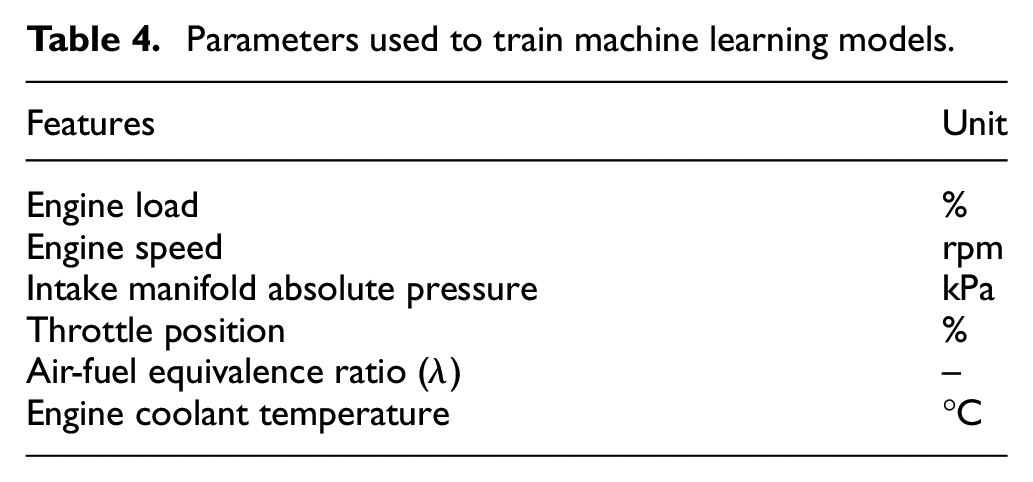
Selected features

Instantaneous fuel consumption models developed in this study are aimed for estimating fuel consumption for fleet vehicles in real-time based on OBD data. The OBD parameters that are used to train these models should be chosen such that they are readily available in all vehicles and directly affect the engine’s instantaneous fuel consumption. The selected parameters are engine load, engine speed, intake manifold absolute pressure (MAP), throttle position, air-fuel equivalence ratio, and engine coolant temperature and are listed in Table 4.

Table 4.

Parameters used to train machine learning models.

Features	Unit
Engine load	%
Engine speed	rpm
Intake manifold absolute pressure	kPa
Throttle position	%
Air-fuel equivalence ratio $(λ)$	–
Engine coolant temperature	°C

The fuel consumption during cold phase – when the engine coolant has not reached to fully warmed-up condition – is more considerable for shorter trips since it accounts for a larger fraction of the overall trip time and distance. Thus it is important to capture the cold start phase in the training data for urban driving fuel consumption models. Coolant temperature from OBD data is used in the training process to represent engine temperature.

Machine learning models

Four machine learning methods were initially implemented for estimating fuel consumption: random forest (RF), artificial neural networks (ANN), support vector machines (SVM), and k-nearest neighbors (KNN). The preliminary investigation revealed that ANN and RF provide the highest accuracy, so they are the focus of the subsequent instantaneous fuel consumption estimation.

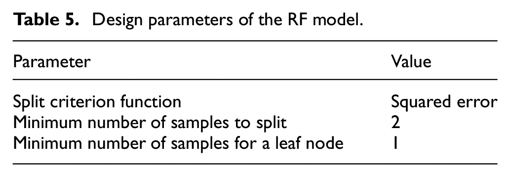
Random forest is a machine learning method that combines the results of multiple decision trees to make more accurate predictions. Each decision tree is built using a random subset of the training data, as well as a random subset of the available features. The final result is determined by averaging the predictions of all decision trees. Figure 4 shows the algorithm of the random forest regression method visually. RF training is resistant to over-fitting since each decision tree learns from a slightly different perspective.³⁹ Additionally, it does not require normalized data and functions well with features that cover a diverse and broad range of feature values.⁴⁰ For the RF method, the design parameters are listed in Table 5 and the number of decision trees for each model is optimized during training and validation.

Figure 4.

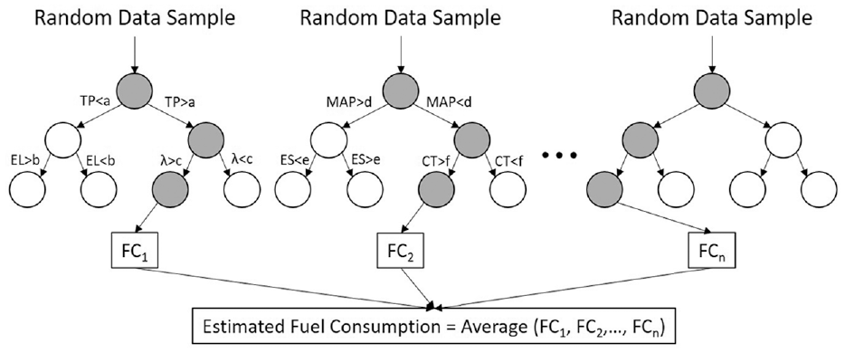
Schematic of the random forest regression algorithm for estimating vehicular instantaneous fuel consumption.

Table 5.

Design parameters of the RF model.

Parameter	Value
Split criterion function	Squared error
Minimum number of samples to split	2
Minimum number of samples for a leaf node	1

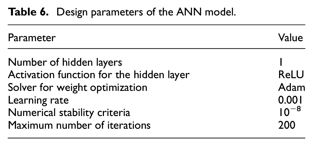
ANN, the other machine learning method used in this study, consists of interconnected nodes, called artificial neurons, organized in layers. These layers typically include an input layer, one or more hidden layers, and an output layer. The connections between neurons have associated weights that are adjusted during the training stage. Each neuron in the input layer represents a feature of the input data, while the output layer typically consists of a single neuron representing the predicted output value. In a hidden layer, each neuron takes inputs from the previous layer and performs a weighted sum of those inputs, followed by an activation function to introduce nonlinearity. The iterative training process continues until the network achieves satisfactory performance.^41,42 Here, an ANN method with one hidden layer and Rectified linear unit (ReLU) as its activation function is used with the design parameters listed in Table 6. Figure 5 is a visual representation of the ANN algorithm. The optimal number of hidden layer neurons for each model is determined during training and validation.

Table 6.

Design parameters of the ANN model.

Parameter	Value
Number of hidden layers	1
Activation function for the hidden layer	ReLU
Solver for weight optimization	Adam
Learning rate	0.001
Numerical stability criteria	10⁻⁸
Maximum number of iterations	200

Figure 5.

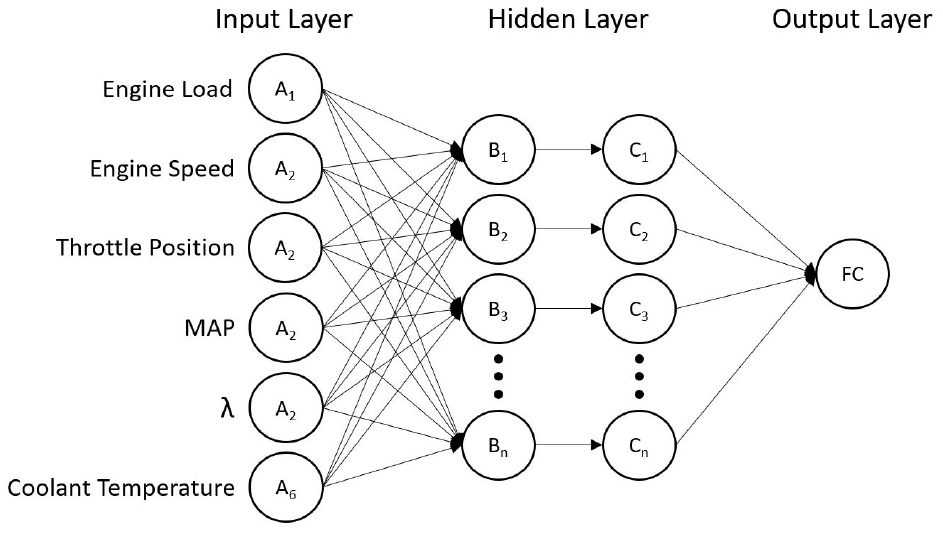
Schematic of the ANN algorithm for estimating vehicular instantaneous fuel consumption.

The hidden layer neurons in Figure 5 are calculated as:

B_{i} = \sum_{j}^{6} W_{j} \cdot A_{j}

(1)

C_{i} = f (B_{i})

(2)

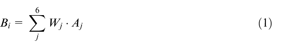
where, $w_{j}$ represents the weights that are adjusted during training and f is the activation function.

The output neuron is calculated as:

FC = \sum_{i}^{n} W_{i} \cdot C_{i}

(3)

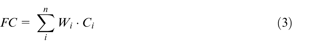
where, FC is fuel consumption, $w_{i}$ represents weights, and n is the number of neurons in the hidden layer which is optimized for each model.

As part of the data preparation procedure for the ANN model training, the data must be normalized because, in contrast to the RF model, the ANN model is sensitive to variations in the range of feature values.⁴³ The normalized data for each feature is formed as:

x_{s} = \frac{x - min (x)}{max (x) - min (x)}

(4)

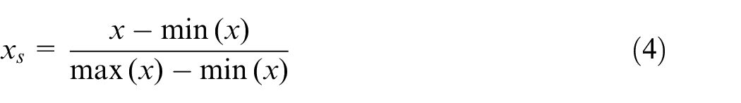
where, x is the actual data and $x_{s}$ is the normalized data between 0 and 1.

To develop the models, the data collected with CANedge2 was divided into two parts. The first part, consisting of 70% of the total data, was used in a five-fold cross-validation method. To do this, 70% of data was divided into five parts and four parts were used for the first repetition and the fifth part was used for validation of the model. The remaining 30% of the data was used to test the two trained machine learning models.

ECU-based calculation

For gasoline engines, there is an ECU-based method for approximating instantaneous fuel consumption that is frequently used in literature and also available in some commercial equipment. This approach calculates fuel flow based on MAF and the ECU-commanded air-fuel ratio. If MAF data is available on the vehicle data, fuel consumption can be estimated as:

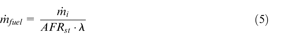
{\overset{\cdot}{m}}_{fuel} = \frac{{\overset{\cdot}{m}}_{i}}{{AFR}_{st} \cdot λ}

(5)

where ${\overset{\cdot}{m}}_{fuel}$ is instantaneous fuel consumption in g/s, ${\overset{\cdot}{m}}_{i}$ is MAF in g/s, AFR_st is the stoichiometric air to fuel ratio (i.e. 14.7), and $λ$ is commanded air-fuel equivalence ratio.^18,19

Even though most modern vehicles have a sensor to measure MAF, not all of them show the MAF value through the OBD acquisition system. If MAF data is not available, it must be calculated using other ECU-reported engine parameters (e.g. intake manifold air temperature, MAP). MAF can be calculated using:

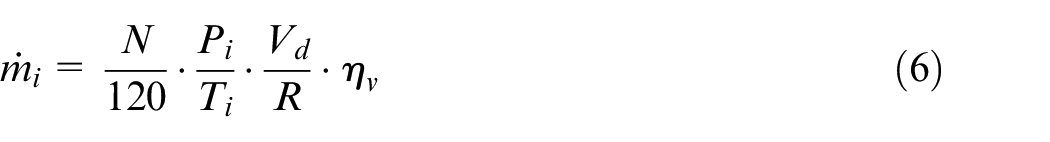
{\overset{\cdot}{m}}_{i} = \frac{N}{120} \cdot \frac{P_{i}}{T_{i}} \cdot \frac{V_{d}}{R} \cdot η_{v}

(6)

where N is engine speed in revolution per minute (rpm), P_i is MAP in kPa, T_i is intake air temperature in K, V_d is engine displacement volume in liter, R is the ambient air gas constant equal to 0.287 J/(g K), and $η_{v}$ is the engine volumetric efficiency.¹⁹ Volumetric efficiency is subjected to change in different operating conditions; however, some studies estimated $η_{v}$ as 0.65 for most of the gasoline engine operating range (0.85 for turbocharged engines) when the $η_{v}$ curve is not available.¹⁸

Since only the Ford Fusion Hybrid MAF data is available among the four selected vehicle types, the outcomes of this method against those from Ford Fusion Hybrid machine learning models are compared. For Ford Escape PHEV and Ford Escape S, MAF measured data is not available via OBD, but is estimated based on other ECU-reported engine parameters. The OBD data of Ford F-350 lack MAF and intake air temperature, so ECU-based fuel consumption calculation would be inaccurate and is not investigated in this study.

Results and discussion

Highway driving models

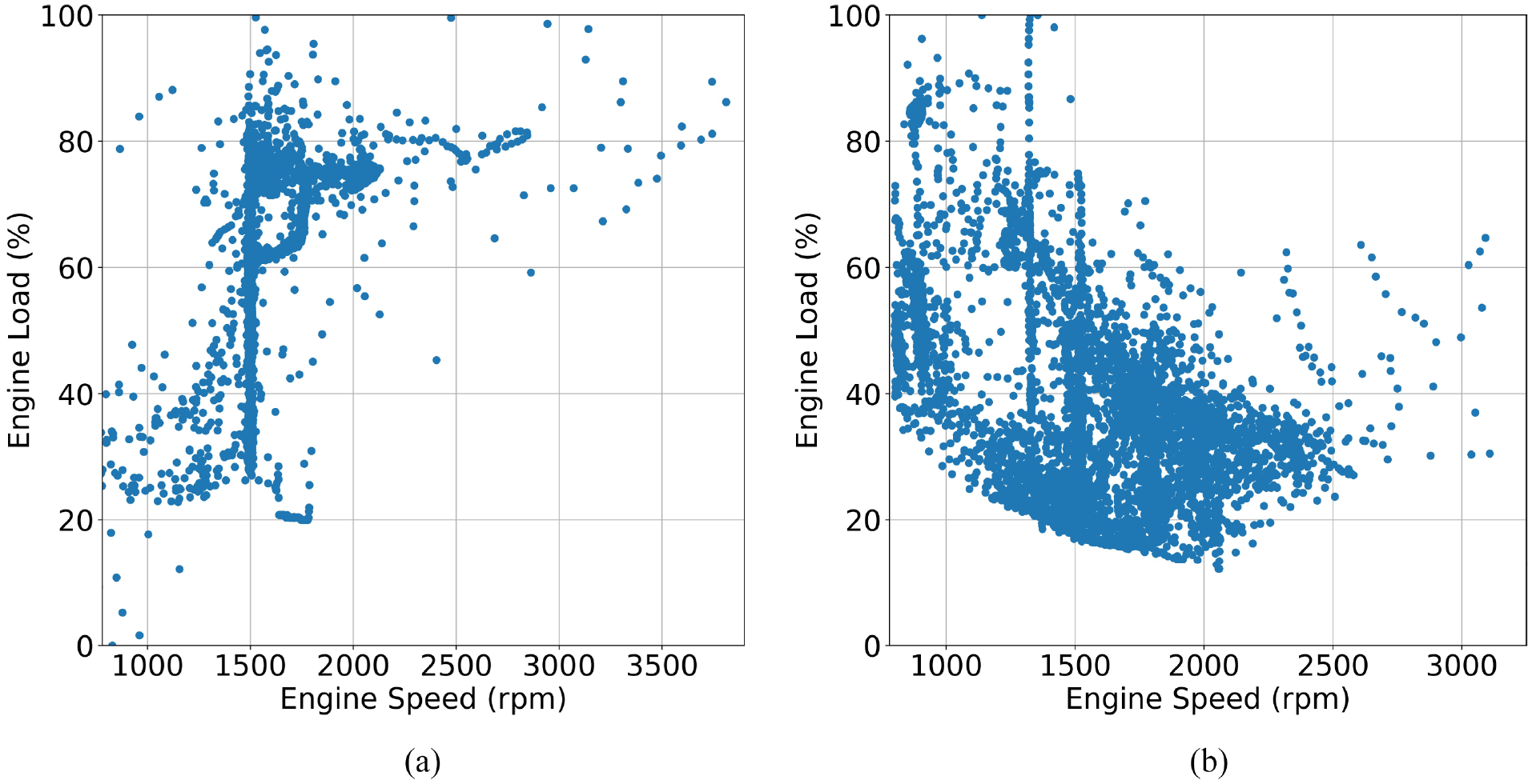
The training data set needs to include all potential operating points to train an accurate fuel consumption model. The two most significant parameters describing the engine operating points are engine load and engine speed. Figure 6 shows the collected data for the drive cycle shown in Figure 1(a) for two vehicles covering a broad engine load (0–100%) and engine speed (idle – 6000 rpm) operating conditions. Ford Fusion is a hybrid electric car, and in some operating conditions the electric battery drives the vehicle instead of the gasoline engine; hence, the engine operating range in Figure 6(a) is less than that in Figure 6(b), for Ford F-350.

Figure 6.

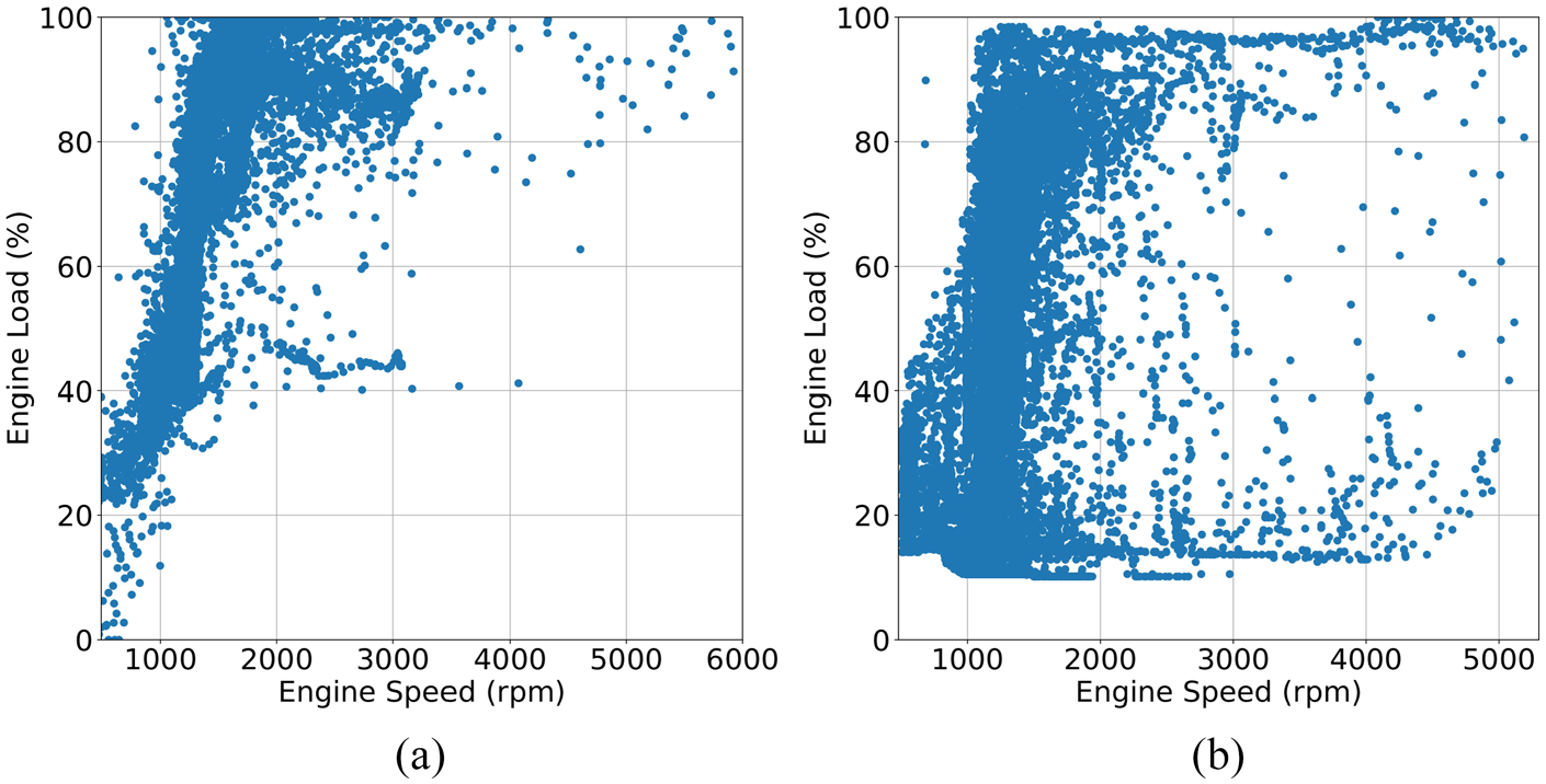
Engine load and speed for the collected vehicle data in the highway driving cycle: (a) Ford Fusion Hybrid and (b) Ford F-350.

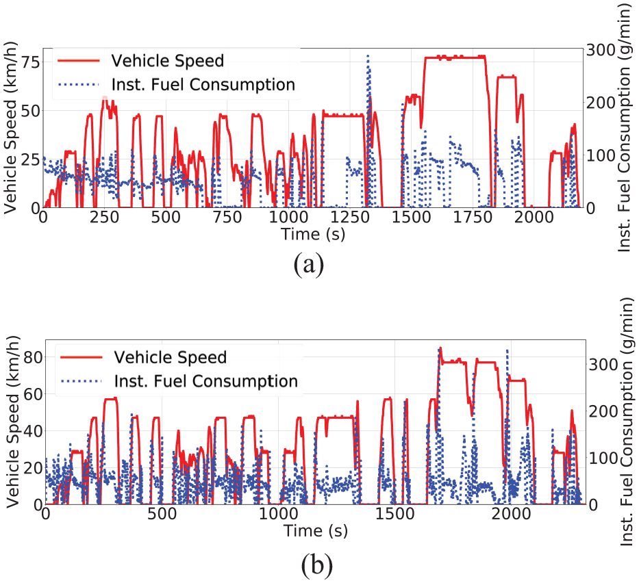
The time series of measured vehicle speed and instantaneous fuel consumption during the trip for both vehicles are shown in Figure 7. Speed profiles demonstrate that the driving cycles of the two vehicles were similar with slight differences due to the volume of traffic on the road at the time of the vehicle testing. Comparing Figure 7(b) with Figure 7(a) shows that heavier traffic during the first 1000 s of the test for Ford F-350 caused more frequent stop/starts, which led to a longer test time on a same path. Driving behavior and operational conditions have a substantial effect on fuel consumption, as shown by the considerable rise and peak in instantaneous fuel consumption that occurs as vehicles accelerate. Ford F-350 consumes more fuel than Ford Fusion Hybrid due to its larger engine and vehicle mass. This fuel consumption difference is clear when comparing Figure 7(b) to 7(a).

Figure 7.

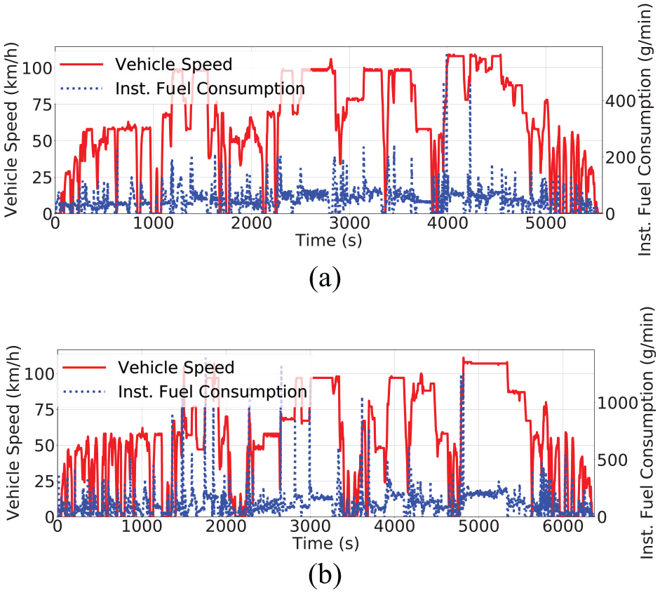
Vehicle speed and measured instantaneous fuel consumption for highway driving cycle as a function of time: (a) Ford Fusion Hybrid and (b) Ford F-350.

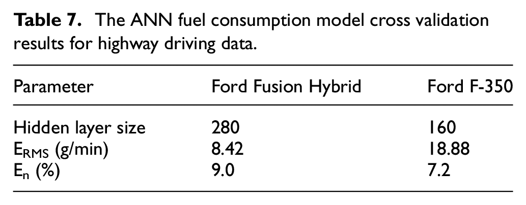
The ANN model cross-validation results are shown in Table 7. The results show that the ANN model can estimate well. The hidden layer size for each model is tuned by minimizing the root mean square error (E_RMS) of the estimated fuel consumption. In addition, normalized mean absolute error (E_n) has been reported for each cross-validation performed on the data set. The reported E_RMS and E_n are the average of validation fold values over five times of training in five-fold cross-validation.

Table 7.

The ANN fuel consumption model cross validation results for highway driving data.

Parameter	Ford Fusion Hybrid	Ford F-350
Hidden layer size	280	160
E_RMS (g/min)	8.42	18.88
E_n (%)	9.0	7.2

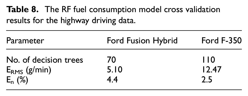
The RF model cross-validation results, listed in Table 8, outperform the ANN model in terms of fuel consumption estimation accuracy for both vehicles. Although the E_RMS of Ford F-350 compared to Ford Fusion Hybrid is higher, it is still very low compared to the fuel flow rate of both vehicle types.

Table 8.

The RF fuel consumption model cross validation results for the highway driving data.

Parameter	Ford Fusion Hybrid	Ford F-350
No. of decision trees	70	110
E_RMS (g/min)	5.10	12.47
E_n (%)	4.4	2.5

Now the models are tested on unseen test data and the RF model has a lower estimation error (E_RMS and E_n) of fuel consumption for both vehicles (Table 9). Plotting measured versus estimated instantaneous fuel consumption is done in Figure 8. A perfect model should line up on the diagonal line. The RF model results (Figure 8(a) and (b)) are closer to the diagonal line than the ANN model results in Figure 8(c) and (d), indicating that the estimated results are closer to the measured values.

Table 9.

Performance of the models on the unseen test data set for highway driving condition.

Model	Vehicle	E_RMS (g/min)	E_n (%)
RF	Ford Fusion Hybrid	4.68	3.9
RF	Ford F-350	11.01	1.8
ANN	Ford Fusion Hybrid	9.71	11.9
ANN	Ford F-350	21.21	9.3
ECU-based	Ford Fusion Hybrid	11.40	16.4

Figure 8.

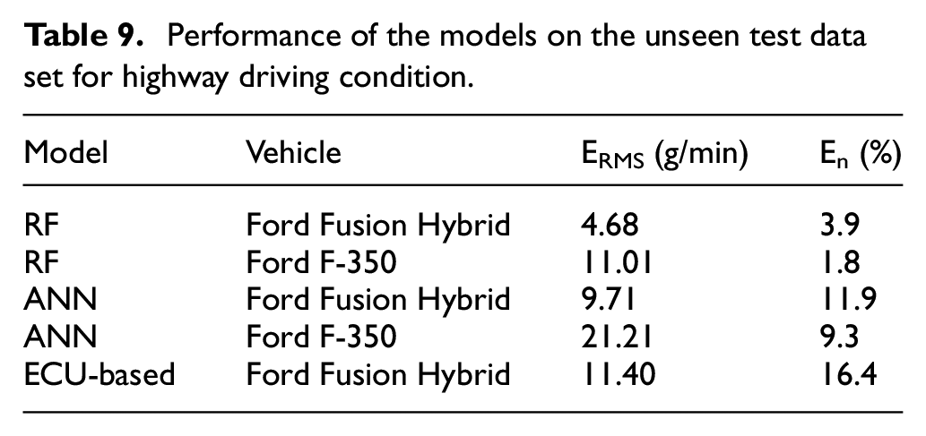
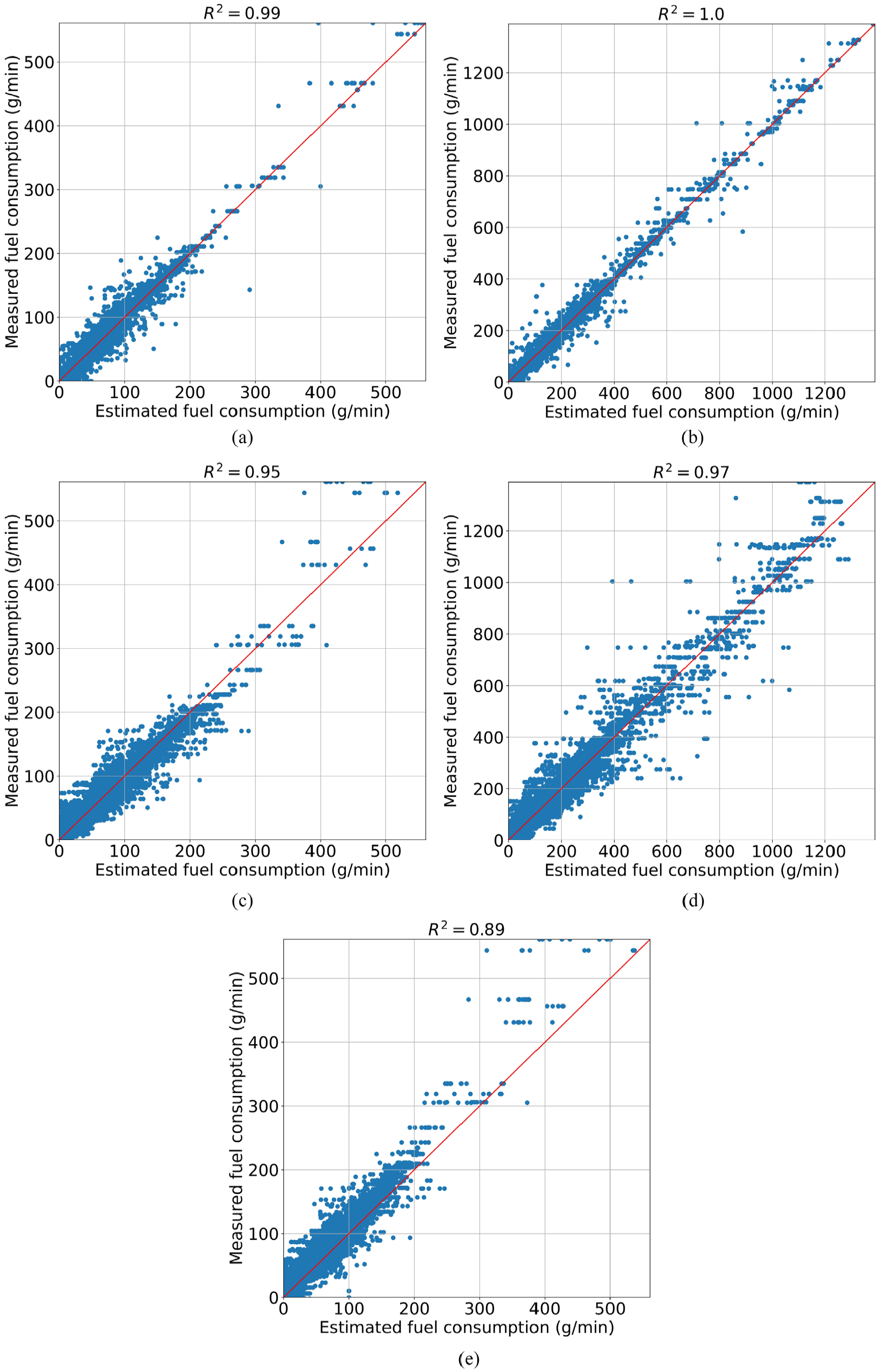
Performance of the RF and ANN models along with the ECU-based calculation for estimating instantaneous fuel consumption for the highway driving test data: (a) RF model – Ford Fusion Hybrid, (b) RF model – Ford F-350, (c) ANN model – Ford Fusion Hybrid, (d) ANN model – Ford F-350, and (e) ECU-based model – Ford Fusion Hybrid.

The results of the Ford Fusion Hybrid ECU-based estimating approach are shown in Figure 8(e) and are less accurate than the two machine learning models.

Urban driving models

Following the same analysis as the highway driving data, the collected data over the urban driving cycle demonstrated in Figure 1(b) for both Ford Escape PHEV and Ford Escape S is shown in Figure 9. The collected data covers a broad engine load (0–100%) and engine speed (idle – 4000 rpm) operating conditions. The urban driving cycle is much shorter than the highway driving cycle and is intended to cover only urban driving conditions, so a more limited engine operating range compared to the highway driving cycle is observed. In addition, since Ford Escape PHEV was operating in a hybrid electric mode, in some operating conditions the electric battery and electric motors drive the vehicle instead of the gasoline engine, so the engine operating range in Figure 9(a) is less than 9(b).

Figure 9.

Engine load and speed for the collected vehicle data in the urban driving cycle: (a) Ford Escape PHEV and (b) Ford Escape S.

The time series of the two vehicles’ instantaneous fuel consumption and speed during the urban driving cycle is shown in Figure 10. Again real road traffic resulted in slight differences in speed profiles. Instantaneous fuel consumption clearly increases when vehicles accelerate so driving behavior and operating conditions have a significant influence on fuel consumption. Ford Escape S has a smaller engine (1.5 l) compared to the Ford Escape PHEV engine (2.5 l), but its 1.5 l engine is turbocharged, so the fuel consumption range between the two vehicles is comparable.

Figure 10.

Vehicle speed and measured instantaneous fuel consumption for urban driving cycle as a function of time: (a) Ford Escape PHEV and (b) Ford Escape S.

As shown in Figure 11, more than a third of the urban trip times is in the cold start period. As shown in Figures 10(a) and 11(a), despite the fact that at the beginning of the trip, there are many stops and the vehicle speed is low and the electric motor must supply the power of the hybrid electric vehicle, but the combustion engine is idling for better powertrain performance. The same pattern happens for Ford Escape S in Figures 10(b) and 11(b), where the engine does not stop operating at the beginning of the trip, even though the vehicle is equipped with the stop/start technology. By doing so, the engine will warm up and the coolant temperature will rise.

Figure 11.

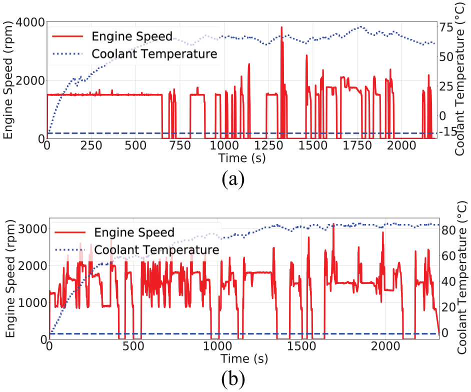
Engine speed and coolant temperature for urban driving cycle as a function of time: (a) Ford Escape PHEV and (b) Ford Escape S.

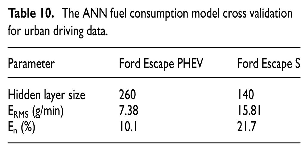
Both vehicles have acceptable ANN validation results with E_n less than 22% for instantaneous fuel consumption, as listed in Table 10. By minimizing the estimated fuel consumption’s E_RMS, the hidden layer size for each model is optimized.

Table 10.

The ANN fuel consumption model cross validation for urban driving data.

Parameter	Ford Escape PHEV	Ford Escape S
Hidden layer size	260	140
E_RMS (g/min)	7.38	15.81
E_n (%)	10.1	21.7

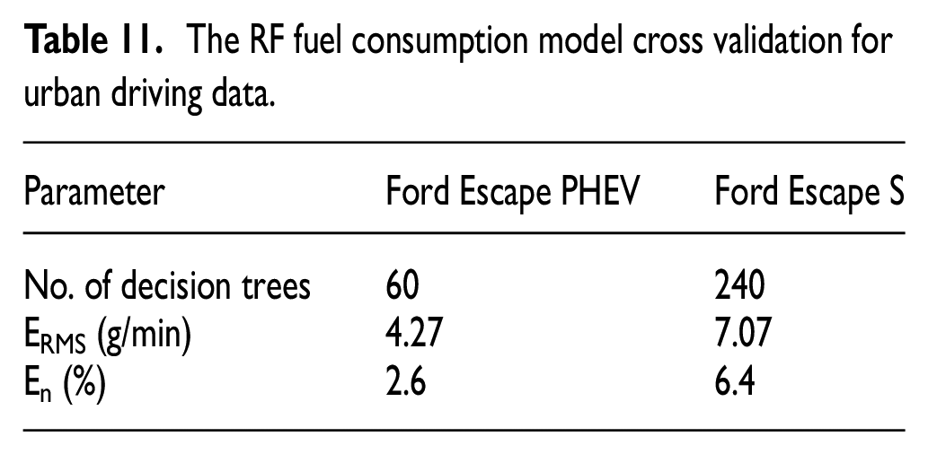
For both vehicles, the RF model error was lower than the ANN model with E_n less than 6.5%, as listed in Table 11.

Table 11.

The RF fuel consumption model cross validation for urban driving data.

Parameter	Ford Escape PHEV	Ford Escape S
No. of decision trees	60	240
E_RMS (g/min)	4.27	7.07
E_n (%)	2.6	6.4

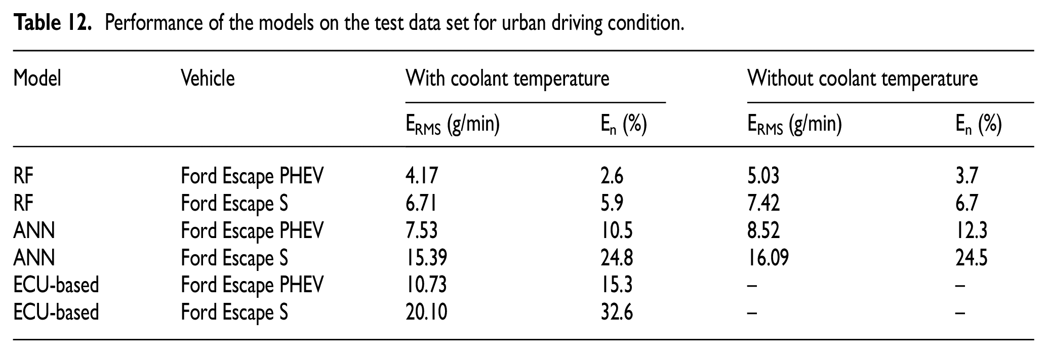
The performance of trained models of the urban driving cycle on the unseen test data is shown in Table 12. Similar to the highway driving models, the RF model provides a more accurate estimation of fuel consumption for both vehicles during the model testing stage. Both E_RMS and E_n show that the RF model produces a precise estimate of fuel consumption (E_RMS < 7 g/min, E_n < 6%). The points of the RF model plots (Figure 12(a) and (b)) are closer to the diagonal line, suggesting that the estimated values are in better agreement with the actual measured data.

Table 12.

Performance of the models on the test data set for urban driving condition.

Model	Vehicle	With coolant temperature		Without coolant temperature
Model	Vehicle	E_RMS (g/min)	E_n (%)	E_RMS (g/min)	E_n (%)
RF	Ford Escape PHEV	4.17	2.6	5.03	3.7
RF	Ford Escape S	6.71	5.9	7.42	6.7
ANN	Ford Escape PHEV	7.53	10.5	8.52	12.3
ANN	Ford Escape S	15.39	24.8	16.09	24.5
ECU-based	Ford Escape PHEV	10.73	15.3	–	–
ECU-based	Ford Escape S	20.10	32.6	–	–

Figure 12.

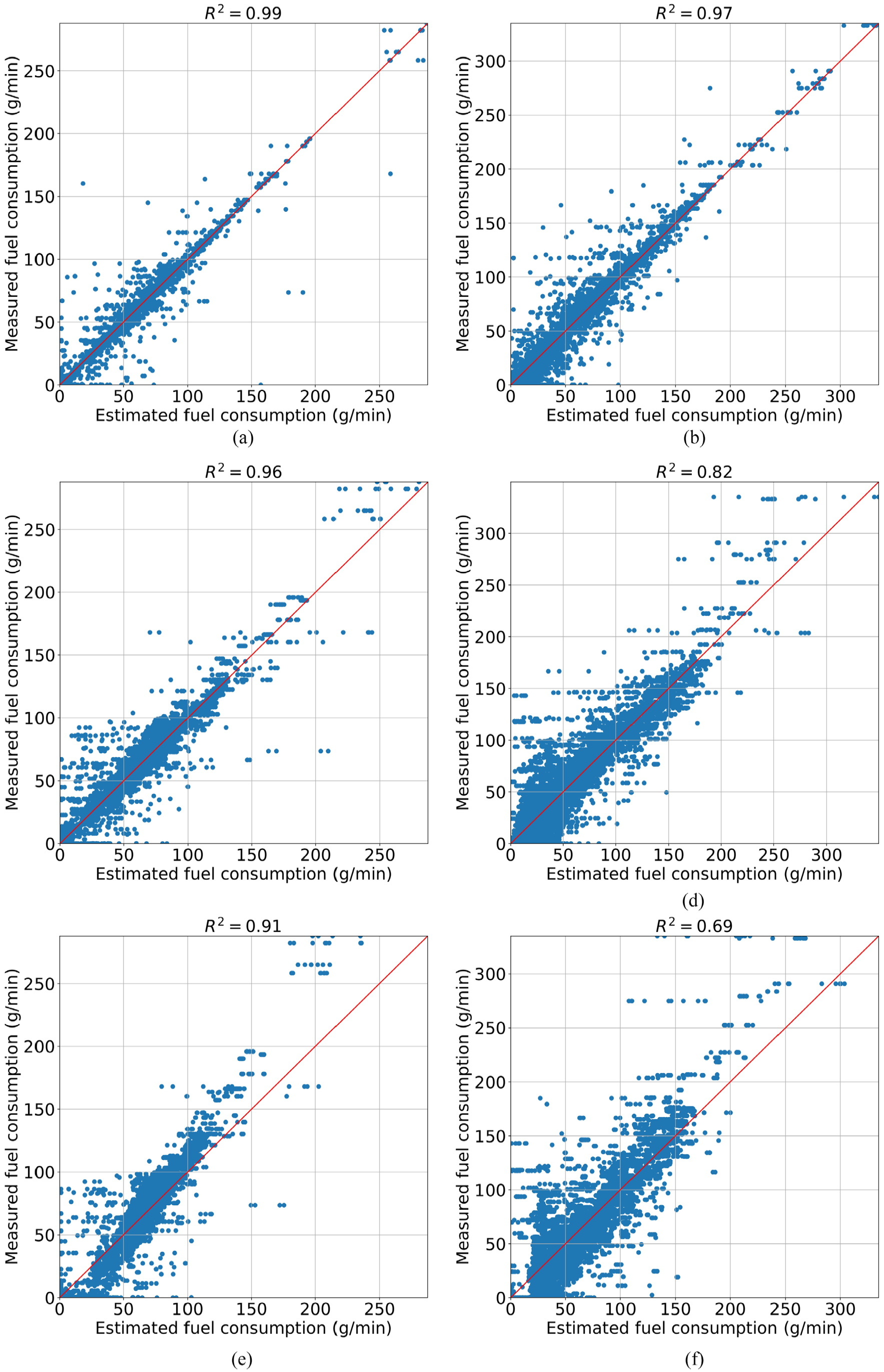
Performance of the RF and ANN models along with the ECU-based calculation for estimating instantaneous fuel consumption for the urban driving test data: (a) RF model – Ford Escape PHEV, (b) RF model – Ford Escape S, (c) ANN model – Ford Escape PHEV, (d) ANN model – Ford Escape S, (e) ECU-based – Ford Escape PHEV, and (f) ECU-based – Ford Escape S.

The performance of RF and ANN can vary depending on the specific dataset, problem complexity, and parameter settings. In this study, RF consistently demonstrated superior estimation accuracy compared to ANN across various datasets. This can be attributed to RF’s effective handling of noisy data and outliers through random sampling during decision tree construction which reduced the impact of individual noisy samples or outliers. Additionally, RF’s hierarchical structure of decision trees allows it to capture complex nonlinear relationships in the data. It automatically learns and represents nonlinear interactions between input variables, contributing to improved estimation accuracy.⁴⁰ In contrast, ANN may require careful tuning of network architecture and activation functions to effectively model nonlinear relationships, particularly when using a simplified ANN structure with only one hidden layer.

As shown in Figure 12(e) and (f) and Table 12, the results of the ECU-based calculation of fuel consumption have the largest error compared to the two machine learning models developed in this study.

As shown in Figure 11, the cold start duration is substantial in the urban driving condition. The coolant temperature data is collected and included among the features to cover the fuel consumption penalty during the warm-up period. Table 12 also exhibits the performance of the models that are trained without the coolant temperature as a feature on the test data set. Comparing these results to the models with coolant temperature as a feature shows that including coolant temperature in the feature set increases the accuracy and reduces the estimation error.

Conclusions

Four different vehicles from the University of Alberta fleet were selected to develop machine learning models to estimate instantaneous fuel consumption based on OBD data. Two different routes, highway and urban driving, were used to collect OBD and fuel consumption data.

For each vehicle, two machine learning models of RF and one-layer ANN were developed to estimate fuel consumption. The OBD parameters used to estimate instantaneous fuel consumption by machine learning models are air/fuel equivalence ratio, throttle position, manifold absolute pressure, engine load, and engine speed. Due to Edmonton’s cold climate, the cold start period of vehicles is long and considerable, particularly in short trips. Therefore, the coolant temperature is added to the features to cover its effect on the fuel consumption penalty in the cold start period. All these OBD parameters are easily accessible through OBD port of most vehicles.

Overall, RF models provided the best estimation accuracy of instantaneous fuel consumption with mean errors of less than 6% in all cases. The one-layer ANN models had a higher error than the RF models. In all the cases, the developed machine learning models had a better estimation performance compared to the instantaneous fuel consumption calculated by measured or estimated MAF data from ECU, which is currently widely used to monitor instantaneous fuel consumption.

Footnotes

Appendix

Acknowledgements

The authors would like to thank Jim Laverty, the manager, and the staff of Transportation Services at the University of Alberta for their support for vehicle instrumentation and testing. The authors also thank Energy Management and Sustainable Operations (EMSO) of the University of Alberta, especially Michael Versteege and Shannon Leblanc for supporting this project.

Declaration of conflicting interests

The author(s) declared no potential conflicts of interest with respect to the research, authorship, and/or publication of this article.

Funding

The author(s) disclosed receipt of the following financial support for the research, authorship, and/or publication of this article: This work was supported by the University of Alberta, Energy Management and Sustainable Operations (EMSO).

ORCID iD

Hamidreza Abediasl

References

Goel

. Fleet telematics: real-time management and planning of commercial vehicle operations. New York, NY: Springer Science & Business Media, 2007.

Malekian

Moloisane

Nair

, et al. Design and implementation of a wireless OBD II fleet management system. IEEE Sens J 2017; 17(4): 1154–1164.

Rojas

Bolaños

Salazar-Cabrera

, et al. Fleet management and control system for medium-sized cities based in intelligent transportation systems: from review to proposal in a city. Electronics 2020; 9(9): 1383.

Tong

Hung

Cheung

. On-road motor vehicle emissions and fuel consumption in urban driving conditions. J Air Waste Manag Assoc 2000; 50(4): 543–554.

Treiber

Kesting

Thiemann

. How much does traffic congestion increase fuel consumption and emissions? Applying a fuel consumption model to the NGSIM trajectory data. In: 87th annual meeting of the Transportation Research Board, Washington, DC, January 2008, vol. 71, pp.1–18.

Lee

Kim

Park

, et al. Effect of the air-conditioning system on the fuel economy in a gasoline engine vehicle. Proc IMechE, Part D: J Automobile Engineering 2013; 227(1): 66–77.

Zhou

Jin

Wang

. A review of vehicle fuel consumption models to evaluate eco-driving and eco-routing. Transp Res D Transp Environ 2016; 49: 203–218.

Miotti

Needell

Ramakrishnan

, et al. Quantifying the impact of driving style changes on light-duty vehicle fuel consumption. Transp Res D Transp Environ 2021; 98: 102918.

Liu

Zhang

, et al. Impact of driving and driver’s operating characteristics on high fuel consumption set based on real-road driving data. Proc IMechE, Part D: J Automobile Engineering. Epub ahead of print 12 January 2023. DOI: 10.1177/09544070221149113.

10.

Zhang

, et al. Real-world emissions and fuel consumption of diesel buses and trucks in Macao: from on-road measurement to policy implications. Atmos Environ 2015; 120: 393–403.

11.

Mansour

Clodic

. Optimized energy management control for the Toyota hybrid system using dynamic programming on a predicted route with short computation time. Int J Autom Technol 2012; 13: 309–324.

12.

Cheng

Nouveliere

Orfila

. A new eco-driving assistance system for a light vehicle: energy management and speed optimization. In: 2013 IEEE intelligent vehicles symposium (IV), Gold Coast, QLD, Australia, 23–26 June 2013, pp.1434–1439. New York: IEEE.

13.

Tu Luu

Nouvelière

Mammar

. Dynamic programming for fuel consumption optimization on light vehicle. IFAC Proc Volumes 2010; 43(7): 372–377.

14.

Meenakshi Nandal

Awasthi

. OBD-II and big data: a powerful combination to solve the issues of automobile care. In: Singh

Asari

Kumar

, et al. (eds) Computational methods and data engineering: proceedings of ICMDE 2020, vol. 2. Singapore: Springer Singapore, 2020, pp.177–189.

15.

Singh

Suryawanshi

Tak

. Smart fleet management system using IoT, computer vision, cloud computing and machine learning technologies. In: 2019 IEEE 5th international conference for convergence in technology (I2CT), Bombay, India, 29–31 March 2019, pp.1–8. New York: IEEE.

16.

Rakopoulos

Giakoumis

. Diesel engine transient operation: principles of operation and simulation analysis. Berlin: Springer, 2009.

17.

Ivarsson

Åslund

Nielsen

. Look-ahead control—consequences of a non-linear fuel map on truck fuel consumption. Proc IMechE, Part D: J Automobile Engineering 2009; 223(10): 1223–1238.

18.

Moradi

Miranda-Moreno

. Vehicular fuel consumption estimation using real-world measures through cascaded machine learning modeling. Transp Res D Transp Environ 2020; 88: 102576.

19.

DeFries

Sabisch

Kishan

, et al. In-use fuel economy and CO₂ emissions measurement using OBD data on US light-duty vehicles. SAE Int J Engines 2014; 7(3): 1382–1396.

20.

Burke

Brace

Hawley

. Critical evaluation of on-engine fuel consumption measurement. Proc IMechE, Part D: J Automobile Engineering 2011; 225(6): 829–844.

21.

Brunton

Kutz

. Data-driven science and engineering: machine learning, dynamical systems, and control. Cambridge: Cambridge University Press, 2022.

22.

Hosseini

Wine

Abediasl

, et al. Knowledge gap on health impact of transportation-related emissions in cold climate cities. Edmonton, AB: University of Alberta, 2021.

23.

Almér

. Machine learning and statistical analysis in fuel consumption prediction for heavy vehicles. Dissertation, KTH, School of Computer Science and Communication, 2015.

24.

Liu

. Development of a predictive system for car fuel consumption using an artificial neural network. Expert Syst Appl 2011; 38(5): 4967–4971.

25.

Liu

. A forecasting system for car fuel consumption using a radial basis function neural network. Expert Syst Appl 2012; 39(2): 1883–1888.

26.

Zeng

Miwa

Morikawa

. Exploring trip fuel consumption by machine learning from GPS and CAN bus data. J East Asia Soc Transp Stud 2015; 11: 906–921.

27.

Gong

Shang

, et al. A comparative study on fuel consumption prediction methods of heavy-duty diesel trucks considering 21 influencing factors. Energies 2021; 14(23): 8106.

28.

Katreddi

Thiruvengadam

. Trip based modeling of fuel consumption in modern heavy-duty vehicles using artificial intelligence. Energies 2021; 14(24): 8592.

29.

Kanarachos

Mathew

Fitzpatrick

. Instantaneous vehicle fuel consumption estimation using smartphones and recurrent neural networks. Expert Syst Appl 2019; 120: 436–447.

30.

Vilaça

Aguiar

Soares

. Estimating fuel consumption from GPS data. In: Pattern recognition and image analysis: 7th Iberian conference, IbPRIA 2015, proceedings, Santiago de Compostela, Spain, 17–19 June 2015, pp.672–682. Cham: Springer International Publishing.

31.

Perrotta

Parry

Neves

. Application of machine learning for fuel consumption modelling of trucks. In: 2017 IEEE international conference on big data (Big Data), Boston, MA, USA, 11–14 December 2017, pp.3810–3815. New York: IEEE.

32.

Wickramanayake

Bandara

. Fuel consumption prediction of fleet vehicles using machine learning: a comparative study. In: 2016 Moratuwa engineering research conference (MERCon), Moratuwa, Sri Lanka, 5–6 April 2016, pp.90–95. New York: IEEE.

33.

Saerens

Rakha

Ahn

, et al. Assessment of alternative polynomial fuel consumption models for use in intelligent transportation systems applications. J Intell Transp Syst 2013; 17(4): 294–303.

34.

Ping

Qin

, et al. Impact of driver behavior on fuel consumption: classification, evaluation and prediction using machine learning. IEEE Access 2019; 7: 78515–78532.

35.

Sun

Chen

Dubey

, et al. Hybrid electric buses fuel consumption prediction based on real-world driving data. Transp Res D Transp Environ 2021; 91: 102637.

36.

Chen

Wang

, et al. Polynomial-based model for estimating instantaneous fuel consumption. Proc IMechE, Part D: J Automobile Engineering. Epub ahead of print 8 August 2022. DOI: 10.1177/0954407022111618.

37.

Pavlovic

Fontaras

Broekaert

, et al. How accurately can we measure vehicle fuel consumption in real world operation? Transp Res D Transp Environ 2021; 90: 102666.

38.

Ansari

Abediasl

Patel

, et al. Estimating instantaneous fuel consumption of vehicles by using machine learning and real-time on-board diagnostics (OBD) data. In: 2022 CSME international congress, Edmonton, AB, Canada, 5–8 June 2022.

39.

Ali

Khan

Ahmad

, et al. Random forests and decision trees. Int J Comput Sci Issues 2012; 9: 272.

40.

Breiman

. Random forests. Mach Learn 2001; 45: 5–32.

41.

Daponte

Grimaldi

. Artificial neural networks in measurements. Measurement 1998; 23(2): 93–115.

42.

Samarasinghe

. Neural networks for applied sciences and engineering: from fundamentals to complex pattern recognition. Boca Raton, FL: CRC Press, 2016.

43.

Nawi

Atomi

Rehman

. The effect of data pre-processing on optimized training of artificial neural networks. Procedia Technol 2013; 11: 32–39.