Sage Journals: Discover world-class research

Abstract

Although simulation-based fatigue analysis is a standard tool adopted in every sector including automotive industry, the design of engine components in automotive and motorsport applications mostly relies on simplified design approaches supported by time-consuming testing programs. This manuscript proposes a new methodology based on individual engine speed damage estimation and engine speed time history combined with Palmgren-Miner linear damage rule to predict the fatigue state of the connecting rod. The track data, engine multibody simulation (AVL Excite^TM) and engine combustion simulation (AVL Boost^TM) are used to generate the initial variable trace that is processed to obtain the block programs. Stress amplitude estimated with finite element analysis (Abaqus) are used to estimate the damage from S-N curve and the cumulative damage is estimated with Palmgren-Miner cumulative damage model. The method proposed is demonstrated using a connecting rod case study and the duty cycle from the race on Sebring international raceway. This work shows the suitability of the approach and the benefit in terms of accuracy in the prediction of the fatigue life.

Keywords

AVL Boost AVL Excite connecting rod internal combustion engine FEA variable amplitude fatigue counting method

Introduction

Engine components experience complex stress loading during service due to the nature of the engine cycle. The combustion cycle includes compressive loads generated by the gas compression and combustion tensile and torsional loads due to the inertia of the components in the engine. The complexity of the requirements is reflected in the manufacturing process, materials and testing protocols adopted for the design. One of the most important parts of the engine is the connecting rod as this links the piston and the crankshaft transforming the vertical motion in torque.¹

The materials used to manufacture engine components range from cast and forged steel to magnesium and beryllium alloys. In terms of material selection of connecting rods, there are several factors to be considered such as density, tensile strength, Young’s Modulus, fatigue behaviour, manufacturing process and cost. Among all the materials, steel is the most prevalent in auto applications and considered as a baseline in comparison. A previous study² focused on powder forging (PF) connecting rod concludes that PF connecting rod displays similar fatigue strength as hot forging SAE 1055 steel connecting rod based on fatigue tests and other factors such as hardness, depth of decarburised layer, metallurgical structure, density and surface roughness, whilst the PF connecting rod shows noticeable advantage in manufacturing process such as reduced energy consumption during manufacturing and cost saving. A later study³ found that as-sintered connecting rod made of mixing material such as steel powder of 4100s, and graphite demonstrates sufficient, although lower, fatigue strength than an equivalent forged steel connecting rod. Niche applications such as racing cars where mass reduction drives the engine design use high performance alloys such as titanium alloys. A FEA study⁴ comparing several similar designs with aluminium alloy 7075-T6, carbon steel 43CrMo4 and titanium alloy Ti-6Al-7V under equivalent load cases suggesting that while the aluminium alloy design achieves the highest weight saving, the safety factor is the lowest with the component experiencing high strain values compared to the other two designs. The titanium alloy, however, features the highest safety factor with some compromise on weight and medium deformation. Without considering the cost and manufacturing process of titanium alloys, this is a very suitable material for connecting rod. Another similar FEA comparison study⁵ using three materials (AISI 4340 steel, aluminium beryllium alloy and titanium alloy) suggested a similar trend in terms of safety factor and deformation and a similar stress distribution and concentration across the component investigated.

The design of connecting rod also involves material selection and fatigue strength. Engine components such as connecting rods and crankshafts experience high cycle fatigue (HCF) and very high cycle fatigue (VHCF).⁶ Although metals with a body-centred cubic lattice structure such as ferritic steels have a fatigue limit and a constant fatigue strength after 10⁶ − 5 × 10⁶ cycles according to related standards,^7,8 some studies^6,9 have pointed out that such assumption is not entirely safe and has led to failures of components subjecting to VHCF during the service life. Thus, in the case of testing data in the VHCF region being unavailable, the study suggests using Woehler curves for calculating the decreasing fatigue strength in the VHCF regions. An additional study¹⁰ investigated several high strength steels and some other non-ferrous metallic materials, deriving a duplex S-N characteristics. Such relations contain two different slopes for an S-N curve, one in the low to high cycle region and another in the very high cycle region. The study points out that although the two curves in both lower and higher cycle regions tend to feature a different primary fracture modes which are surface-initiated fracture and interior inclusion-initiated fracture respectively, each curve possesses multiple other fracture modes such as grain boundary cracking, machining flaw-induced fracture, interior small shrinkage and weak microstructure that may overlap in some regions and happen in parallel.

The geometrical design of a connecting rod can be divided into major considerations, namely the cap and the shank as Figure 1 demonstrates. The cap is the lower part of the cylinder shape located on the crank end which is commonly connected to the shank of the conrod through two bolts. Analytical approach to examine multiple different cross section designs in the cap region of connecting rod were presented by Baldini et al.¹¹ including the validation with results from FEA. Based on this study, regardless of the applied load, the bending stress in the cap region is mainly affected by the cap cross sectional geometry and initial gap between the crankpin and the cap. Furthermore, normal stress in the cap region is approximately 10 times higher than the bending stress.

Figure 1.

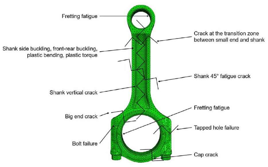
Common failure locations on the connecting rod.¹²

For the shank, there are two designs that are prevalent in automotive industries namely I-beam and H-beam. An FEA study¹³ comparing the two designs with identical weight, meshing method and materials under equivalent load conditions has shown that the stress field is different with a different location of the peak stress. The FEA results for the H-beam profile show that the maximum von Mises stress is 15.7% lower and peak displacement is 43.1% lower compared to the I-beam design. However, I-beam profile is more dominant in the current market due to its simpler and cheaper manufacturing process.

The first attempt to estimate the stress field in the connecting rod and predict its residual fatigue life was presented by Webster et al.¹⁴ This study presented a 3D model of the entire component under tension and compression highlighting the limitation in the complex stress distribution at the connecting rod bolt section. The four locations with significant stress levels were the upper section of the cap end, the interface region of the bolt section and the lower rib, the interface region of the lower rib and the shaft and the conrod bolt end. Another study² presented the experimental results of mechanical testing on connecting rod highlighting the link between fatigue strength and hardness.

Based on the stress analysis, different parts of the connecting rod are subject to different magnitudes of stress.¹⁵ More importantly, the stress types and amplitudes which are two major factors on fatigue analysis vary across the connecting rod. Experimental studies have shown that both piston and crank end pin surfaces are subject to fretting fatigue due to the high frequency of reciprocating frictional contacts,¹⁶ while the connecting rod shank region is often failed due to the tensile stress.¹⁷ For the I-beam design, typically fatigue failure point is in correspondence of four specific notches well reported in the literature.¹⁸ Several studies including¹² have identified multiple locations and its corresponding fracture modes in connecting rod (Figure 1).

While engine dyno test can reliably assess the fatigue life of engine components such as connecting rod in a control environment, test duration and cost make this approach unsuitable for product development. For this reason, stress life and strain life methods, adopted for high cycle and low cycle fatigue analysis respectively, are the preferred approaches. However, life methods use experimental data, usually derived from constant amplitude load on standard specimens, to define correlation between number of cycles and stress or strain.¹⁹ Finite element modelling can overcome this problem, providing a more accurate estimation of the stress or strain field experienced by the component under service load conditions. The load time history is used as input to estimate the stress field in the component. However, in real life applications engine components experience variable amplitude stress-time histories with amplitude changing over time. This requires the use of specific approaches to extract block programs with cycles by cycle counting approaches.²⁰ While a standard counting method such as rainflow method is widely used in automotive and aerospace applications,²¹ a study suggests an alternative method to count main cycle, secondary cycle and carrier cycle separately.²² Although this method is more accurate, it involves more complicated automated calculation during the counting process.

The counting methods transform the spectrum with variable amplitude load or stress time history in a series of blocks. Each of them is characterised by a given amplitude so that the particular block can be dealt with as a constant amplitude load acting on the component under investigation. The analysis of each block provides the damage produced and the combination of the damage produced by each block represents the total damage. Several damage models including linear such as Palmgren-Miner²³ and non-linear such as Macro and Starkey load-dependant damage theory and Kwofie and Rahbar model based on fatigue driving stress²⁴ have been proposed. The linear approach is usually the most used even though it neglects key factors such as load sequence.

The approach proposed in this article is discussed with the use of a case study applying track data to derive discretized rpm histograms, engine combustion simulation (AVL Boost^TM) to acquire cylinder pressure trace of each rpm bin, engine multibody simulation (AVL Excite^TM) and FEA software (Abaqus) to generate the load cycles of each rpm bin. For the fatigue life prediction, since the load cycle for each rpm power stoke is relatively simple giving that the cycle in each rpm bin features same tensile and compressive load, the counting algorithm can be simplified greatly, and maximum and minimum values can be identified easily. Combining the obtained load cycles, track data, material S-N curve and cumulative damage model, fatigue damage caused by each load cycle at each engine speed can be multiplied by the corresponding number of that load cycles per lap on track. Therefore, a cumulative fatigue damage per lap and fatigue life in terms of number of laps can be calculated.

For demonstrating purpose, this study created an AVL Boost^TM model of the GM LT1 engine and a single cylinder AVL Excite^TM model to evaluate the fatigue life of a given connecting rod model shank region based on the material properties of EN DD12 steel and track tested data from a vehicle using the aforementioned engine at Sebring International Raceway.

Methodology

The methodology can be summarised in the following individual sections as shown in Figure 2. The input information includes the track data, CAD model and material properties for this method. The arrow indicates the sequence of the procedure. Each section will be explained separately in the following sections.

Figure 2.

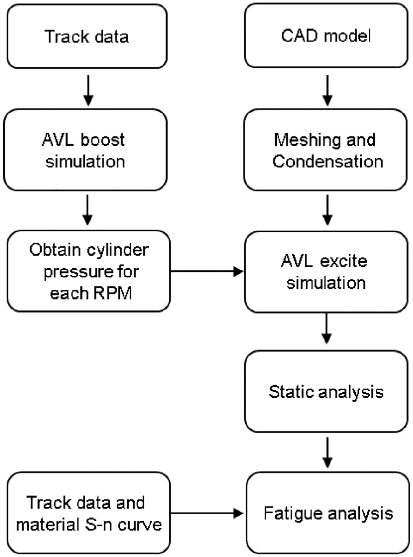
Overview of the procedure of this method.

Track data processing

An engine speed trace with a sampling rate of 83.33 Hz in the time domain was acquired from the GM Vehicle Performance Data Recorder (Parts number: 84437246) and GM LT1 engine. The data was converted into time histogram with a bin width of 200 rpm and a total of 20 bins from 2500 to 6500 rpm using Cosworth Pi Toolbox. A total of three fastest laps was selected through three sessions. The time versus rpm histogram is further converted into number of Power strokes at each rpm per lap. The average of the three laps is taken as shown in Figure 3.

Figure 3.

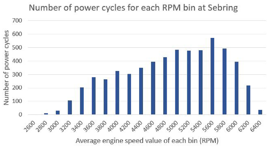
Histogram of average power cycles of each rpm bin.

Equation (1) is used to convert rpm into power strokes assuming the model is a 4-stroke engine, meaning every 2-crankshaft rotation for 1 power stroke cycle. For each bin, the middle rpm was used for the calculation.

No . of Powerstroke cycle = \frac{time (\sec) \cdot (\frac{RPM}{60})}{2}

(1)

AVL Boost^TM model

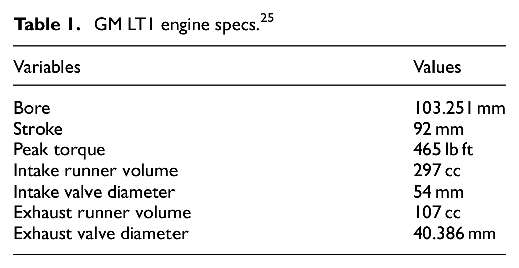
In order to obtain the cylinder pressure curve in the angle domain for each rpm bin, an AVL Boost^TM model is created based on the natural aspirated V8 GM LT1 engine used in the car from which the previously mentioned rpm data originates. The general specifications of the model are set to match with the published data of the engine, which are summarised in Table 1.

Table 1.

GM LT1 engine specs.²⁵

Variables	Values
Bore	103.251 mm
Stroke	92 mm
Peak torque	465 Ib ft
Intake runner volume	297 cc
Intake valve diameter	54 mm
Exhaust runner volume	107 cc
Exhaust valve diameter	40.386 mm

Given the relation between torque output and BMEP (Brake Mean Effective Pressure), the output torque curve from the simulation of AVL Boost^TM model and dyno testing of the physical engine were used to validate the output cylinder pressure curve from the AVL Boost TM (as an exponent) model as shown in Figure 4. The focus of the study being the methodology, the aim with the AVL Boost^TM model was to achieve the same peak torque as the engine dyno data and to generate relevant pressure curves. Engine parameters such as ignition timing are fixed instead of being varied with engine speed hence the discrepancies between both curves in Figure 4.

Figure 4.

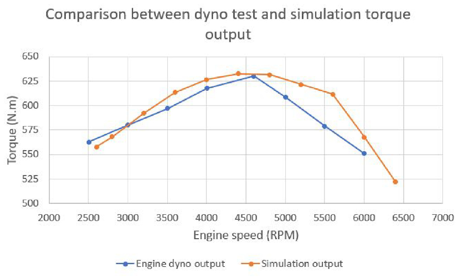
Torque curve comparison between AVL Boost^TM model and LT1 engine dyno test.²⁶

The model was then used to generate cylinder pressure curve for each rpm bin from the track data. The simulated cylinder pressure curve at 2600, 4600 and 6400 rpm is shown as Figure 5.

Figure 5.

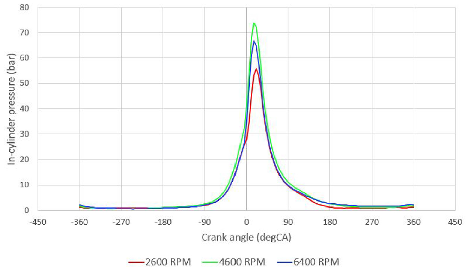
Cylinder pressure traces in crank angle domain at 2600, 4600 and 6400 rpm.

Meshing and condensation

The FE model of the connecting rod used in this study is shown in Figure 6. Material is defined as EN DD12 steel with density of 7.85 g/cm³, Young’s modulus of 207 GPa and Poisson’s ratio of 0.29. The length and bore diameters are from the stock connecting rod design of the engine with the same I-beam profile. The model contains 80,601 nodes and 44,796 elements including 40,398 quadratic tetrahedral elements of type C3D10 (no hourglass control, faster resolution) and 4398 modified tetrahedral elements of type C3D10M (hourglass control making it suitable for contact surfaces, better accuracy, require more computational power) and assumes linear elastic material model behaviour. Following mesh sensitivity, the minimum element size is 1.64 mm while the maximum is 3.47 mm.

Figure 6.

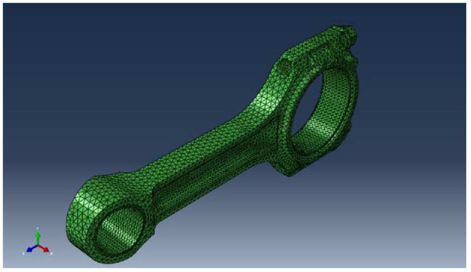
Mesh of the connecting rod used in the study.

Based on the meshed profile, a membrane for the piston end pin and crank end pin respectively are created with surface-based TIE Constraint. A 5-percent tolerance for each membrane slave surface is defined, followed by membrane meshing for both ends. Then, a condensation task is created in AVL Excite^TM based on Craig-Bampton method.²⁷ This method combines motion of boundary points with modes of the structure to reduce the size of finite element model. Following the AVL Excite^TM tutorial to condense the connecting rod model, the boundary DOFs were defined as following: all nodes on the membrane of both ends (DOFs 2 and 3), on the connecting rod centre of gravity (DOFs 1–6) and eight other nodes on axial joint connection (DOF 1).

AVL Excite^TM model

The assembly of the model in AVL Excite^TM is shown in Figure 7.

Figure 7.

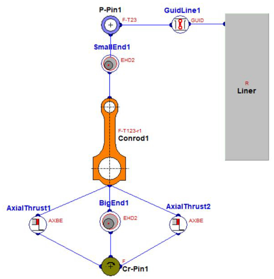
AVL Excite^TM diagram of the model assembly.

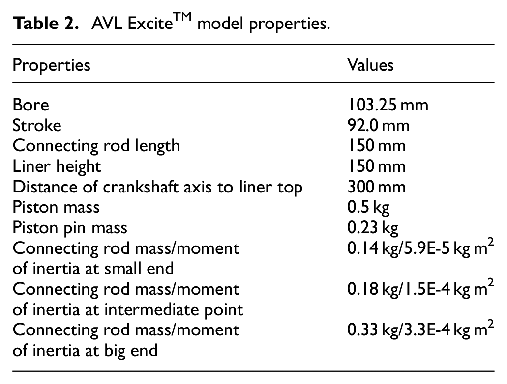
The pressure curve for each rpm bin generated from AVL Boost^TM is used in AVL Excite^TM to evaluate compression load for a given rpm as a global parameter. SAE 5W-30 (with dynamic viscosity of 0.009 Pa s at 100°C) is selected for engine oil as used in the stock engine. Geometry and inertia are shown in Table 2.

Table 2.

AVL Excite^TM model properties.

Properties	Values
Bore	103.25 mm
Stroke	92.0 mm
Connecting rod length	150 mm
Liner height	150 mm
Distance of crankshaft axis to liner top	300 mm
Piston mass	0.5 kg
Piston pin mass	0.23 kg
Connecting rod mass/moment of inertia at small end	0.14 kg/5.9E-5 kg m²
Connecting rod mass/moment of inertia at intermediate point	0.18 kg/1.5E-4 kg m²
Connecting rod mass/moment of inertia at big end	0.33 kg/3.3E-4 kg m²

Journals were created at both crank and piston ends to simulate bearing and applied force. For the journal, the same material properties as the connecting rod were used. While the piston liner is defined as rigid and crank pin is defined with circular motion with no active DOF, piston pins are allowed 2 active DOFs and connecting rod is set with 4 active DOFs, with all directions of motions and 1 degree of rotations. The bearing contact condition at both ends is defined as elastohydrodynamics (EHD)²⁸ with asperity contact, which applies Greenwood/Tripp model²⁹ and uses averaged Reynolds equation. Rayleigh damping is applied on the connecting rod material damping given that research has shown it improves the stability of calculated results.³⁰ The simulation was performed over two power stroke cycles (1440° crank angle) with step size of 0.00125° crank angle (AVL Excite^TM default value) for each rpm bin, where 0° and 720° crank angle are corresponding to piston at TDC between exhaust and intake strokes.

Static analysis

A linear static analysis is performed in AVL Excite^TM considering the EHD pressure load and acceleration as inertial load. A step size of 10° CA is used due to computer storage limitation for the linear static analysis. The second power cycle (from 720° CA to 1440° CA) from the simulation of each rpm is used to ensure convergence of the stress output results. Nodal displacement and stress are obtained and von Mises and stress values in the longitudinal direction in each step angle are calculated. The change of stress magnitudes and direction with respect to rpm is also investigated. Further, a separate case of stress distribution is created based on no combustion load and open valves (i.e. cylinder pressure equals to atmospheric pressure) model to examine stress due to cyclic load and rpm relations.

Fatigue analysis

The methodology discussed in this work does not account for thermal, size and surface finish effects since the expected temperature for the connecting rod would not significantly change the stiffness and the size and surface finish effect would only linearly increase the maximum stress without any impact on the approach. It is also worth noting that this approach is developed for high cycle fatigue whereby plasticity is negligible.

This study focuses on the shank region of the connecting rod because the pin part of the connecting rod is subject to different fatigue modes such as fretting.¹² For the demonstration purpose, a conservative assumption was made that the cut off stress amplitudes is 10⁷ number of cycles, which is noticeably higher than what suggested by the Eurocode 3 guideline.⁷

S-N curves are based on the material properties provided by Granta EDU pack 2021 and are modified according to Basquin and Coffin-Manson approximations.³¹ For the application of different stress ratios Granta EDU pack 2021 applies modified Goodman’s relation³¹ to update the original S-N curve.

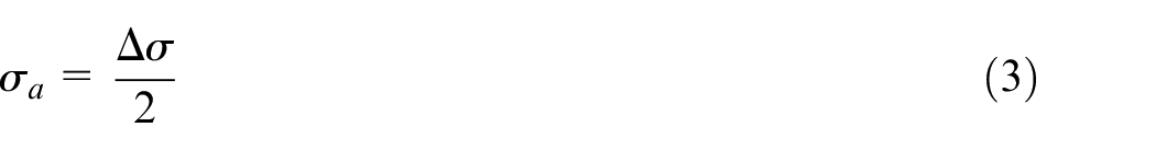
Stress range $Δ σ$ is defined as:

Δ σ = σ_{\max} - σ_{\min}

(2)

Where $σ_{\max}$ and $σ_{\min}$ are the maximum and minimum stresses in the stress cycle respectively and stress amplitude $σ_{a}$ is given by:

σ_{a} = \frac{Δ σ}{2}

(3)

Moreover, the stress ratio is given by:

R = \frac{σ_{\min}}{σ_{\max}}

(4)

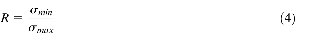
Given the stress amplitude in one stress cycle, the S-N curve based on stress ratio can be used to obtain fatigue life (i.e. number of cycles to failures) for each rpm case. Stress amplitudes that correspond to number of cycles higher than 10⁷ are neglected.

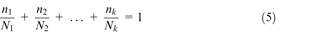
Palmgren-Miner linear cumulative damage model was then used,²³ and it can be expressed by:

\frac{n_{1}}{N_{1}} + \frac{n_{2}}{N_{2}} + \dots + \frac{n_{k}}{N_{k}} = 1

(5)

where $n_{1}, n_{2} \dots n_{k}$ represent cycles at specific stress level according to the track data and $N_{1}, N_{2} \dots N_{k}$ indicate fatigue life in cycles at the same stress amplitudes according to the S-N curves. Combining with the lap data, percentage of damage of each rpm bin and percentage of damage from each lap can be estimated. Each fraction represents a percentage of damage contributed by that specific stress level.

The total lap number ( $N_{lap}$ ) achievable before failure is therefore given by:

N_{lap} = \frac{1}{(\frac{n_{@ 2600}}{N_{@ 2600}} + \frac{n_{@ 2800}}{N_{@ 2800}} + \dots + \frac{n_{@ 6400}}{N_{@ 6400}})}

(6)

Where $n_{@ 2600}, n_{@ 2800} \dots n_{@ 6400}$ represent cycles at specific rpm per lap and $N_{@ 2600}, N_{@ 2800} \dots N_{@ 6400}$ indicate fatigue life in cycles at the specific rpm.

Results and discussions

FEA and stress analysis

The results for three specific engine speeds, namely 2600, 4600 and 6400 rpm are used to demonstrate that these three cases contain all the extreme input values through the entire rpm range. Notably, 2600 rpm experiences the lowest combustion and cyclic loads. 4600 rpm features the highest combustion load while 6400 rpm faces the highest cyclic load as shown in Figure 8. Peaks of cyclic and combustion loads are respectively experienced at 0°CA and between 15 and 20°CA depending on the engine speed (0°CA corresponds to TDC between compression and expansion strokes).

Figure 8.

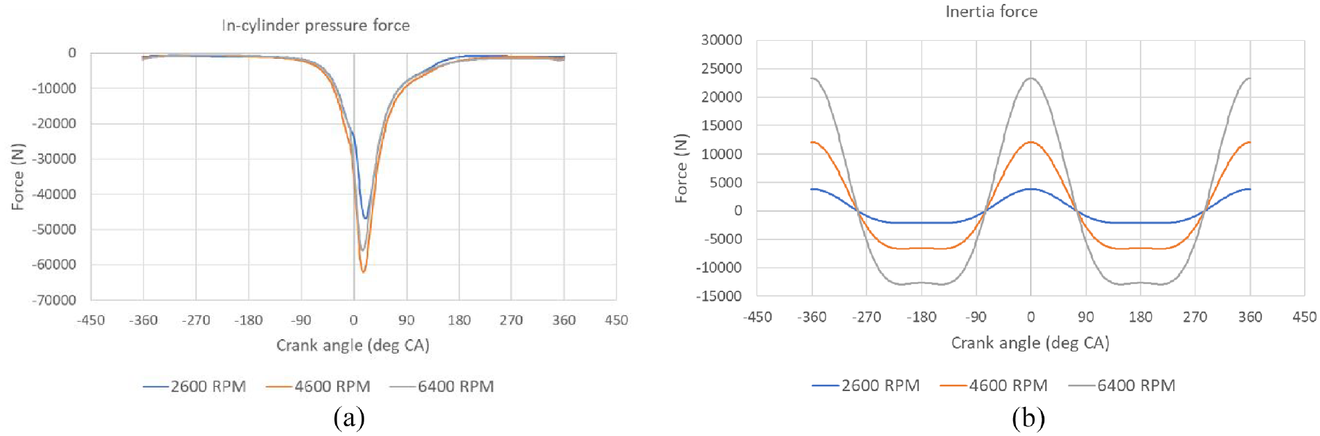
Combustion induced force (a) and inertia force (b) acting on the conrod at 2600, 4600 and 6400 rpm.

According to Figure 8, the combustion-induced force on the conrod does not evolve linearly with engine speed in results of different combustion start and air/fuel ratios for each engine speed to match the torque presented in Figure 4. On the contrary, it can be seen that the inertia force acting on the conrod increases with engine speed, that is, with angular velocity, because of the higher deceleration/acceleration on the piston end.

When combining combustion-induced and inertia forces, it is possible to estimate the axial force experienced by the conrod (Figure 9). It can be highlighted that as for the inertia force, the peak tension force of the total axial force increases with engine speed whereas the peak compression force varies differently because of the difference in peak in-cylinder pressures.

Figure 9.

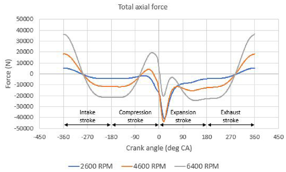
Total axial force experience by the conrod at 2600, 4600 and 6400 rpm.

For 4600 rpm, despite the cyclic load leading to higher tension force than that for 2600 rpm around TDC in consequence of the higher engine speed, the significantly higher combustion load leads to a higher compression force resulting in a higher compressive load faced by the conrod. The combustion load has increased faster than the cyclic load.

On the contrary, 6400 rpm experiences both higher maximum and minimum peaks as the combustion force has reduced compared to 4600 rpm and the cyclic load has further increased.

On the contrary to what was observed in another study,³² the simulations carried out for this research project show that the stress range is not constant over all engine speeds. The maximum stress increases with engine speed as a result of the higher cyclic load but the minimum stress does not evolve as linearly because of the difference in peak-cylinder pressures with engine speed.

As shown in Figure 10, the maximum stress increases faster than the minimum one, leading to an increase in stress range. The main difference between this study and the work presented by Shenoy and Fatemi³² is the consideration of combustion load variation with engine speed. Thanks to the simulations ran with AVL Boost^TM, the AVL Excite^TM model was provided with a specific pressure trace for each engine speed whereas Shenoy and Fatemi³² only had access to one which was applied to all cases.

Figure 10.

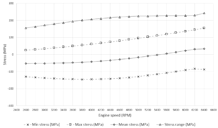
Minimum, maximin, mean stresses and stress range evolution with engine speed.

Because of this difference in maximum and minimum stress evolutions, 2600 and 4600 rpm will experience nearly identical peak compression stresses and the conrod at 4600 rpm will be under tension during the compression stroke whereas at 2600 rpm, it will only face very low compression stress (Figure 11).

Figure 11.

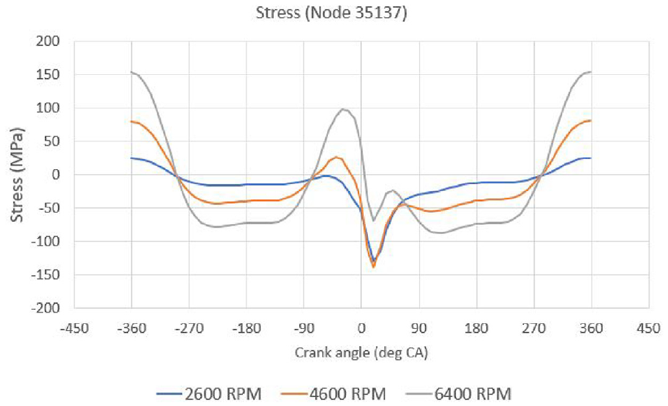
Stress experienced at node 35137 of the conrod for 2600, 4600 and 6400 rpm.

Fatigue analysis

The FEA results have shown a consistent stress concentration spot, which is the interface region between the lower rib and the shank, with the studies that also feature the I-beam connecting rod.^13,14

Based on overall stress amplitude and ratio of the entire range of rpm and cycles number of each rpm, failure initiation point is found to be at node 35137 (Figure 12) on the surface of the transition region between the piston/small end and the shank where the surface is a curved sharp edge, and the sectional area is reduced to the approximate minimum. The amplitude is marginally higher within the low rpm region at another node in the transition region between the big end and the shank on the surface of a similar curved sharp edge where sectional area is also close to the minimum. It is then discarded given that the cumulative damage is significantly less. A plot of that the longitudinal stress amplitude on node 35137 is are shown in Figure 11.

Figure 12.

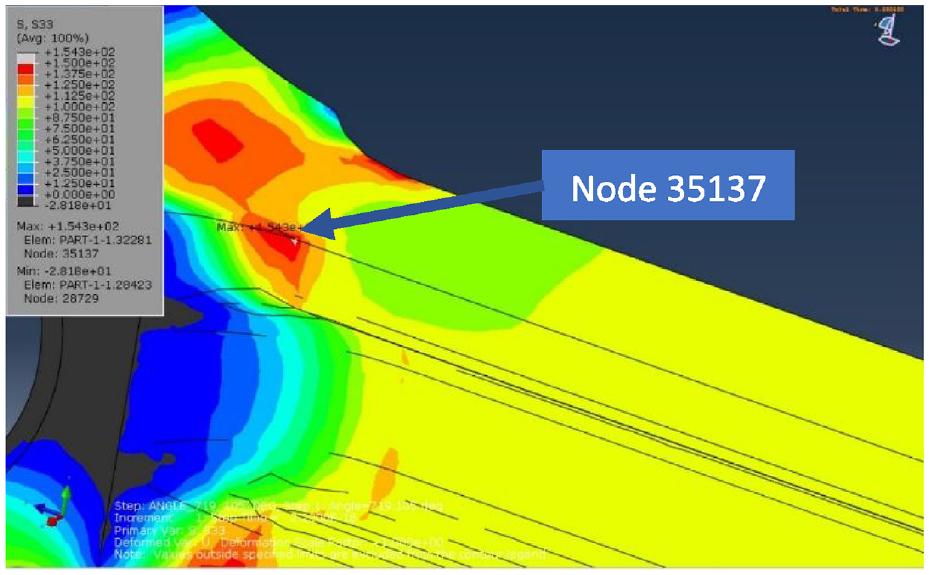
Location of node 35137 on the zoomed in contour plot.

After counting the number of stress cycles on node 35137 of each rpm case, the combining results from the track data and each rpm stress cycle can be summarised as Figure 13.

Figure 13.

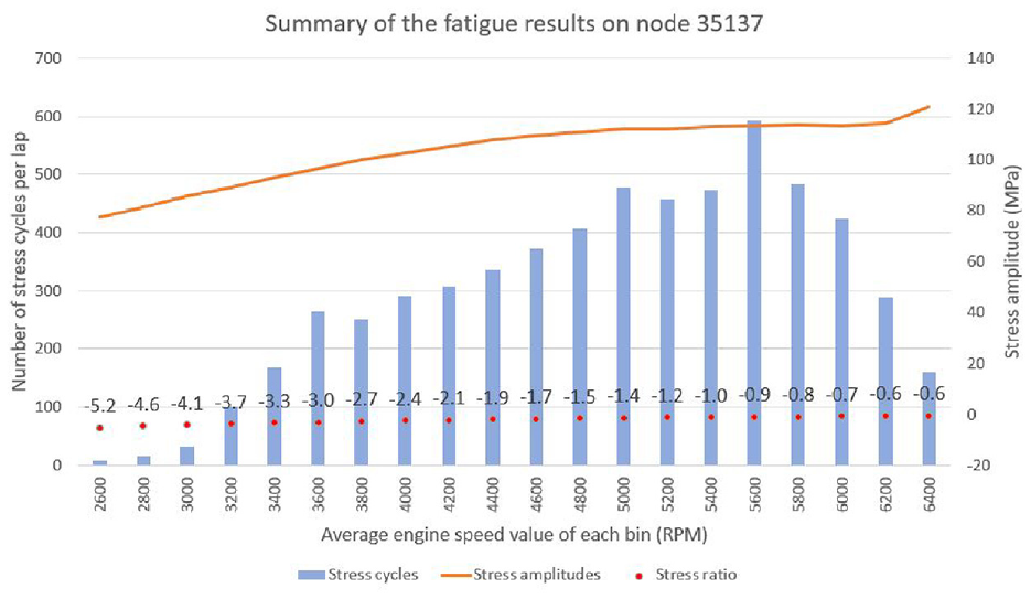
Summary of longitudinal stress results on node 35137 across the rpm range per lap.

Based on Figure 10 and S-N curve, the number of cycles until failures is obtained as shown in Figure 14. The number of stress cycles until failures are assumed to be infinite when exceed 10⁷, therefore lower rpm are not shown in the Figure 14.

Figure 14.

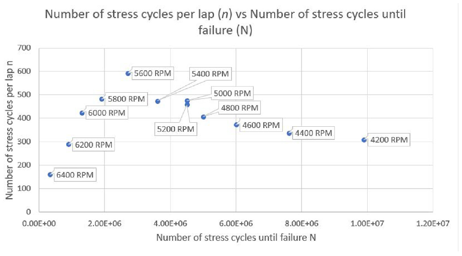
Number of stress cycles per laps versus number of cycles until failures.

Using equation (5), values in Figure 14 can be converted into percent of damage per lap as shown in Figure 15.

Figure 15.

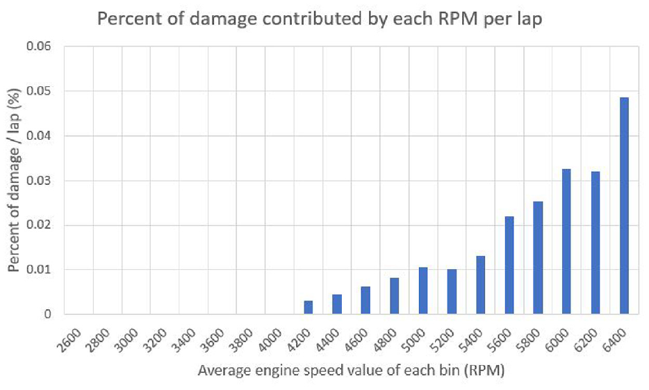
Percentage of damage contributed by each rpm per lap.

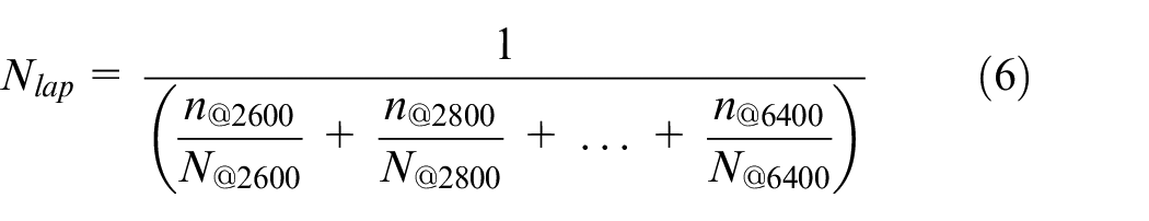
By substituting these values into equation (6), the estimation suggests a total operation life of 462 laps before failures, which roughly equals to three 12-h endurance race in GTE PRO class at Sebring.

Based on Figure 10, it can be observed that the stress amplitude is constantly increasing as the engine speed increases. Figure 8 shows the dominance of the tension side (i.e. positive stress values from amplitudes graph) both in terms of magnitude and time in tension zone due to cyclic load. According to the study¹² which reviews common conrod failures, the transition region between the piston pin and the shank region is commonly subject to fatigue crack. The fracture location based on the experiment and FEA mentioned in the study demonstrate the failure initiation point on the surface of the transition region between the piston/small end and the shank.

Node 35137 from Figure 12 matches the surface crack initiation points shown in the experiment and the stress concentrating spot from FEA in the study. After comparison, it is possible to predict the surface initiate fracture will also be displayed on the FEA predicted spot of the connecting rod model covered in the study.

In Figure 13, the rate of increment of stress amplitude curve (orange line) possesses a declining trend in the lower to mid rpm range due to the cancelling between compression and tension during combustion cycle. However, the stress amplitude of the last rpm case namely 6400 rpm noticeably increased. The sudden disappearance of cancelling effect is caused by the increasing rate of cyclic load growth and sudden reduction of the combustion peak pressure. Physically, the sudden drop of the combustion pressure is due to the rpm limiter, which is set at 6200 rpm, restricting fuel supply. While there is no rpm limiter in simulation setup, the matching of torque curve in this region between the simulation model and the physical engine as shown in Figure 4 can be used to mimic this phenomenon given that the torque curve is directly related to combustion pressure as well. From Figure 13, it can be observed that the stress ratio is consistently rising, which means that the tensile stress is more dominant in the stress cycle and that the number of cycles to failures on the updated S-N curve is reduced compared to the original one. Hence, it can be speculated that fatigue damage per rpm in the higher rpm region will be drastically greater due to all three factors which are higher stress amplitudes, number of stress cycles per lap and stress ratios. Given Figure 13, it is simple to identify the main influence factor on fatigue damage percentage for each rpm, either high number of stress cycles or large stress amplitude. The partial damage of each rpm bin per lap is shown in Figure 15. Although the number of occurrences of the 6400 rpm peak is considerably lower than that of the region between 3600 and 6200 rpm, the corresponding fatigue damage per lap is considerably higher and equal to 0.0485% per lap. As a result, it is possible to conclude that the higher stress amplitude, due to the scale and slope of S-N curve in this demonstration, plays a dominant role in contributing to the total fatigue damage.

Evaluation of the methodology

The method suggested in this study demonstrates several advantages over conventional methods in determining the fatigue cycle of connecting rod:

It is mostly based on simulation except for material properties and some limited track data. Compared with other studies where combustion loads are obtained through testing and strain amplitude needs to be measured, this method can be used on a computer with a licence of several software if material and track data is presented.

It is relatively simple. Some studies have used rainflow-counting algorithm or more complicated counting method to process the stress amplitude throughout the entire working duration. It would be equivalent to measure the strain on connecting rod throughout entire race. In this study, by discretising the rpm, stress cycle can be easily obtained, and amplitude can be directly counted.

It is flexible. The method is a combination of multiple software and physics models. Similar software is interchangeable, a variety of effects for fatigue calculation can be considered and different models for various level of accuracy or scenarios can be applied in each stage.

However, this methodology does have areas that can be improved and limitations:

More information from the track data can be used to improve the accuracy of the method. For example, the braking pressure or throttle times traced data can be incorporated into the model as well as engine cylinder pressure under different throttle position or braking. By separating the conrod damage under different throttle positions, it will improve the accuracy of the cumulative fatigue damage.

The application of testing data such as material properties might not be accurate compared to the physical model given that multiple factors should be considered such as defects inside the connecting rod during manufacturing process. And different materials and manufacturing process will have different degrees of impact on the product defects properties,¹⁵ leading to different accuracy on the fatigue life predictions.

It does not support other applications outside of motorsports. Track data such as time trace of rpm and brake pressure is usually obtainable only on the race cars equipped with racing data loggers. Also, circuit racing is a very repetitive event, meaning the rpm trace exhibits a high level of similarity between each lap, leading to a reasonably identical cumulative fatigue damage of each lap. Automotive applications, on the other hand, could be based on pre-determined driving cycles or recorded cycles such as WLTP.

Since this methodology is new, there is not much validation on this topic. Although software tools and physics models mostly have been tested and validated, the combination effect of all and other factors which might influence the result are still unknown.

Conclusion

The study has successfully applied the purposed methodology and completed the original three objectives. An engine model in AVL Boost^TM and a connecting rod model in AVL Excite^TM were created. Combustion pressure data from AVL Boost^TM were been applied during the calculation of the connecting rod stress in AVL Excite^TM. FEA stress simulation results of each rpm bins were acquired (each bin has a width of 200 rpm ranged from 2600 to 6400 rpm). Tension induced by cyclic loading and compression induced by combustion load were found to have interference, reducing the final stress on the connecting rod during the combustion phase. The stress amplitudes tend to increase as rpm rises. Track data was obtained and calculation of the fatigue damage from each rpm bin on the connecting rod based on linear cumulative fatigue damage model and estimation of the connecting rod life in terms of lap was performed. The connecting rod used in the simulation was found to last 462 laps based on the predictions, corresponding to 36 h of racing. Majority of fatigue damage per cycle is mostly contributed by the higher rpm cases. Notably the 6400 rpm case contributes to the highest amount of fatigue damage per lap. Overall, the innovative methodology has simplified the traditional fatigue counting algorithm yet still needs validation and detailed study on various applications in the future.

Footnotes

Declaration of conflicting interests

The author(s) declared no potential conflicts of interest with respect to the research, authorship, and/or publication of this article.

Funding

The author(s) received no financial support for the research, authorship, and/or publication of this article.

ORCID iD

Marzio Grasso

References

Heywood

. Internal combustion engine fundamentals. 1st ed. New York, NY: McGraw Hill, 1988.

Imahashi

Tsumuki

Nagare

. Development of powder-forged connecting rods. SAE technical paper 841221, 1984.

Suzuki

Toyama

Konda

. Development of as-sintered P/M connecting rod for automobiles. SAE technical paper 880168, 1988.

Haider

Kumar

Chowdhury

, et al. Design and structural analysis of connecting rod. Int Res J Eng Technol 2018; 5(5): 282–285.

Nitturkar

Kalshetti

Nadaf

. Design and analysis of connecting rod using different materials. Int Res J Eng Technol 2020; 7(3): 1011–1017.

Sonsino

. Course of SN-curves especially in the high-cycle fatigue regime with regard to component design and safety. Int J Fatigue 2007; 29(12): 2246–2258.

CEN European Committee for Standardization. Eurocode 3. Design of steel structures, part 19: fatigue, https://www.phd.eng.br/wp-content/uploads/2015/12/en.1993.1.9.2005-1.pdf (1993, accessed 5 June 2023).

FKM Forschungskuratorium Maschinenbau. Analytical strength assessment of components. 6th revised ed. VDMA Verlag, 2012.

Pyttel

Schwerdt

Berger

. Very high cycle fatigue – is there a fatigue limit? Int J Fatigue 2011; 33(1): 49–58.

10.

Sakai

Nakagawa

Oguma

, et al. A review on fatigue fracture modes of structural metallic materials in very high cycle regime. Int J Fatigue 2016; 93(2): 339–351.

11.

Baldini

Strozzi

Bertocchi

, et al. Stresses in the cap of a connecting rod. Eng Fail Anal 2021; 129: 105693.

12.

Strozzi

Baldini

Giacopini

, et al. A repertoire of failures in connecting rods for internal combustion engines, and indications on traditional and advanced design methods. Eng Fail Anal 2016; 60: 20–39.

13.

Frătiţa

Uzuneanu

Balanescu

. About I-beam versus H-beam connecting rod design using Inventor Autodesk 2018. IOP Conf Ser Mater Sci Eng 2018; 444(7): 072008.

14.

Webster

Coffell

Alfaro

. A three dimensional finite element analysis of a high speed diesel engine Con rod. SAE technical paper 831322, 1983.

15.

Afzal

Fatemi

. A comparative study of fatigue behavior and life predictions of forged steel and PM connecting rods. SAE technical paper 2004-01-1529, 2004.

16.

Wright

. Testing automotive materials and components. Warrendale, PA: Society of Automotive Engineers (SAE), 1993.

17.

Lee

, et al. Buckling sensitivity of a connecting rod to the shank sectional area reduction. Mater Des 2010; 31(6): 2796–2803.

18.

Kandreegula

Paroche

Mukherjee

, et al. Fatigue analysis and validation of fracture split connecting rod for value engineering using 1D and 3D simulation tools. SAE technical paper 2016-01-1735, 2016.

19.

Cecchel

Razavi

Mega

, et al. Fatigue testing and end of life investigation of a topology optimized connecting rod fabricated via selective laser melting. Int J Fatigue 2022; 164: 107134.

20.

Alain Nussbaumer

. Fatigue design of steel and composite structures. Berlin: Wiley, 2012.

21.

Amzallag

Gerey

Robert

, et al. Standardization of the rainflow counting method for fatigue analysis. Int J Fatigue 1994; 16(4): 287–293.

22.

Xiong

Shenoi

. A load history generation approach for full-scale accelerated fatigue tests. Eng Fract Mech 2008; 75(10): 3226–3243.

23.

Miner

. Cumulative damage in fatigue. J Appl Mech 1945; 12(3): A159–A164.

24.

Hectors

Waele

. Cumulative damage and life prediction models for high-cycle fatigue of metals: a review. Metals 2021; 11(2): 204.

25.

OnAllCylinders Staff. LT1 6.2L engine specs: performance, bore & stroke, cylinder heads, cam specs & more. onallcylinders, https://www.onallcylinders.com/2018/02/08/lt1-2014-present-engine-specs-performance-bore-stroke-cylinder-heads-cam-specs-more/ (2018, accessed 5 June 2023).

26.

Magda

. New LT1 engine rated at 460 horsepower. enginelabs, https://www.enginelabs.com/news/new-lt1-engine-rated-at-460-horsepower/ (2013, accessed 5 June 2023).

27.

Bampton

Craig

Jr . Coupling of substructures for dynamic analyses. AIAA J 1968; 6: 1313–1319.

28.

Fantino

Godet

Frêne

. Dynamic behaviour of an elastic connecting–rod bearing – theoretical study. SAE technical paper 830307, 1983.

29.

Greenwood

Tripp

. The contact of two nominally flat rough surfaces. Proc Inst Mech Eng 1970; 185(1): 625–633.

30.

Bai

Chen

Liang

, et al. Simulation analysis of shot peening on the surface of high-load connecting rod. IOP Conf Ser Mater Sci Eng 2020; 892(1): 012074.

31.

DiMatteo

. ASM handbook: fatigue and fracture. Volume 19. Lampman

(ed.). Materials Park, OH: ASM International, 1996.

32.

Shenoy

Fatemi

. Dynamic analysis of loads and stresses in connecting rods. Proc IMechE, Part C: J Mechanical Engineering Science 2006; 220(5): 615–624.

On a numerical methodology to assess the fatigue life of connecting rods

Abstract

Keywords

Introduction

Methodology

Track data processing

AVL BoostTM model

Meshing and condensation

AVL ExciteTM model

Static analysis

Fatigue analysis

Results and discussions

FEA and stress analysis

Fatigue analysis

Evaluation of the methodology

Conclusion

Footnotes

Declaration of conflicting interests

Funding

ORCID iD

References

AVL Boost^TM model

AVL Excite^TM model