
Abstract
This paper presents a real-time driver characterisation algorithm that models the driver based on 10 parameters governing their control of vehicle longitudinal speed and acceleration. It utilises an open-loop longitudinal model in conjunction with an Unscented Kalman Filter (UKF). The algorithm can operate in real-time using velocity and acceleration measurements, in addition to a-priori knowledge of the path curvature and road features such as speed limit locations. The UKF also enables a system identification process to estimate average response of each driver. These identified parameters are subsequently fitted to independent measures of fuel economy and safety to demonstrate possible uses for the characterisations. In addition to the comprehensive characterisation of the drivers’ behaviour the work is also novel in its unique approach to identifying time-based parameters within a time-varying dynamic system (UKF). Possible applications include insurance black box assessments of driver aggressiveness and safety, and in autonomous driving algorithms by providing a model to closely replicate the specific driving styles of various users.
Keywords
Introduction
Driver behaviour is challenging to model as it is a function of many factors. These include mood, cognitive load, physical health, alertness level, aggressiveness and relative safety as factors specific to the driver, as well as external factors such as weather and traffic conditions. Some of these factors are constant or slowly varying, whereas others vary within each journey.
MacAdam’s significant work in modelling and understanding the human driver placed the greatest importance of the driving control task on the visual and vestibular sensory channels. 1 The former accounts for over 90% of the control task, while in some scenarios, such as during cornering or in conditions of heavy crosswind, the vestibular channel is dominant. This is also supported by other studies,2,3 and is consistent with the general consensus of a requirement for driver preview and an internal model of the vehicle’s response, as explored in MacAdam, 4 Ungoren and Peng 5 and Zhang et al. 6
The task of driving requires simultaneous lateral and longitudinal control actions; multiple algorithms have been presented for lateral control,5,7–9 but relatively few for longitudinal control. Most of those lateral control works concentrate on accurate path-following or modelling near-limit race driving, whereas the average driver on the road neither uses the limit nor aims to accurately follow path centre line. Most papers considering longitudinal control on the other hand tends to focus on car following and motorway driving, which is quite different to the natural speed control behaviour of people on country roads in the absence of traffic.
In Kiencke et al., 9 the authors split the model into several modes – straight line driving, cornering and the deceleration and acceleration events pertaining to them. While they go into great detail of modelling the discrete events that make up the task of longitudinal driving, they do not provide a means of characterising drivers. With regards to driver speed choice, there are multiple studies that have shown drivers rely on their vestibular system to limit lateral acceleration levels in corners of significant curvature, and that this relationship is nonlinear. 10 Another study 11 found that drivers tend to slow down earlier for corners of higher curvature. This paper will present a new approach to modelling these events and also go on to demonstrate how the parameters governing this model can be correlated to over-arching (global) characteristics of the driver.
There are a number of factors that can be used to predict driver behaviour that have been identified (e.g. in Weir and Chao 12 ), however, only attitude/personality and experience are considered to be ‘constant’ in the long-term, as opposed to driver state, task demand and situational awareness, which can change even within the same journey. Furthermore, multiple studies,12,13 show that there are inter and intra-personal differences between drivers and their behaviour.
In terms of driver characterisation, there are two main areas of focus – incident prevention and emissions reduction. Both of these are heavily related to identifying aggressive driver behaviour, and multiple approaches (along with their combinations) have been proposed; anomaly detection, acceleration threshold and machine learning methods.
Identifying driver behaviour is typically done by counting the number of ‘aggressive’ events per drive or per unit distance. 14 Event detection can be achieved through various statistical (Partial Least Squares Regression, Gaussian Mixture Model or K Nearest Neighbors 15 ) or machine learning methods16,17 that identify patterns in longitudinal acceleration or find outliers that can be classified as anomalous. Threshold-based methods, on the other hand, make use of fixed or variable thresholds for acceleration to detect to count aggressive driving events – for example harsh braking, aggressive turns. However, these are very dependent on road type, traffic conditions, traffic flow and weather.
Aggressive driving is by definition at higher speed and accelerations, which also require more energy and, hence, fuel. Consequently in Edwards, 18 the author uses a specific dynamics metric in an attempt to quantify driver aggressiveness. The author highlights the differences between real-world driving emissions and drive-cycle test emissions that stem from a variety of factors as a need for the development and consequent matching of ‘aggressiveness’ of those drives and cycles, respectively.
The algorithm given here is based on a naturalistic driving study, designed to characterise drivers in terms of their speed control in the specific environment of driving on single carriageway, winding country roads in the absence of other traffic. The focus is deliberately narrow; this environment is unique in exposing differences in driving style that are entirely driver-dependent. The purpose is to capture those aspects of vehicle speed control that best characterise differences such as driver confidence, aggression (as expressed by energy wastefulness) and attitude to safety (factors that are difficult to determine in other more constrained environments such as driving in traffic or on clear highways). The method provides continuous identification of the driver, so there are numerous benefits: To infer over-arching performance, for example in terms of driver safety (for insurance purposes), energy efficiency and to determine significant changes of behaviour over time. It also allows for future autonomous systems to better replicate speed control behaviour that the driver finds agreeable.
The paper considers collection of test data and the formulation of a model for forward speed and acceleration in Section 1. Section 2 provides a Kalman filter structure for real-time evolution of those model parameters. Section 3 then considers the use of the same filter for system identification, by repeated iteration over the recorded data, to provide an average characterisation of each driver over an hour of driving. Finally, Section 4 illustrates the capacity of the collected parameters to estimate two examples of over-arching driver performance using a formal regression technique.
Test data
Twenty-two drivers took part in two drives on separate days, with each session lasting around 90 min, in a Ford Focus RS with manual gearbox. A wide range of driver demographic was captured, with ages ranging from 20 to 85; the drivers are ordered by age in Appendix 1. The route concentrated on B class country roads around the village of Bagworth in Leicestershire, UK. These are relatively narrow bidirectional single carriageway roads of between 5 and 6.5 m overall width, with the majority (about 75%) de-restricted to the national speed limit of 60 mph. Significantly the road visibility and frequency of corners prevents drivers from driving at such a high speed, so we observe a range of maximum speeds and cornering acceleration behaviours. Roads through villages had speed limits of 30 or 40 mph. The route has a diversity of road features in corners of varying curvature, straights of different length in addition to narrower and wider sections. A complete map is shown in Figure 1.
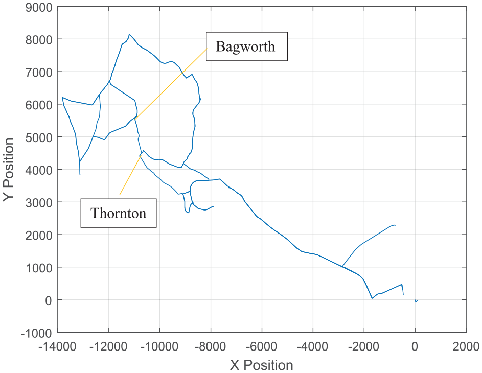
Complete map of routes traversed.
The drivers were asked to drive freely, as they would if they were alone, with the data logger seated in the back and communication restricted to the provision of directions when necessary. Recording was restricted to free driving with no car following, though this information was purposefully kept from the driver to avoid influence on their behaviour. Position, velocity and acceleration data were collected using an OXTS 3200 INS, and steer angle was collected from the vehicle CAN.
The longitudinal model
A time-varying (situation-dependent) open-loop particle model is adopted to represent speed and acceleration events that the driver performs while driving on straight sections, through corners of varying severity, and under the influence of speed limits. The aim is for the model to capture the significant timings and magnitudes of acceleration events, along with straight-line speed, thereby identifying the driving style in a set of well conditioned parameters that can be adapted using a real-time Unscented Kalman Filter. To do this it is assumed that the curvature of the path ahead and the positions of speed limits are known to the model a-priori, and also that the instantaneous position of the vehicle on (and its direction along) the path is known continuously. Current GPS mapping algorithms could be used for the latter, or the position on the path could be estimated by combining the longitudinal model of this paper with the lateral model of Best. 19
For clarity in the discussion below, the model is split into separate accelerations A1– A4 based on situational context, and the parameters that will be adapted by the UKF are printed in bold.
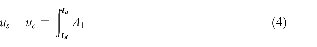
Cornering, A1
The main behaviour that is both characteristic and necessary of all drivers is deceleration on the approach to a corner, combined with acceleration out of it. All but the most novice drivers have developed an internal model of the vehicle response, which combines with their personal driving experience and style to instinctively target a speed through the corner, based on their perception of corner severity, that results in a level of lateral acceleration that they are comfortable with.
The observation in Best 20 is that most drivers target a consistent lateral acceleration, usually in the range of 2–4 m/s 2 . This makes for a good means of parametrising driving style. However, the magnitudes and timings of the deceleration and acceleration manoeuvres before and after the corner apex also give insight into the urgency and style of driving.
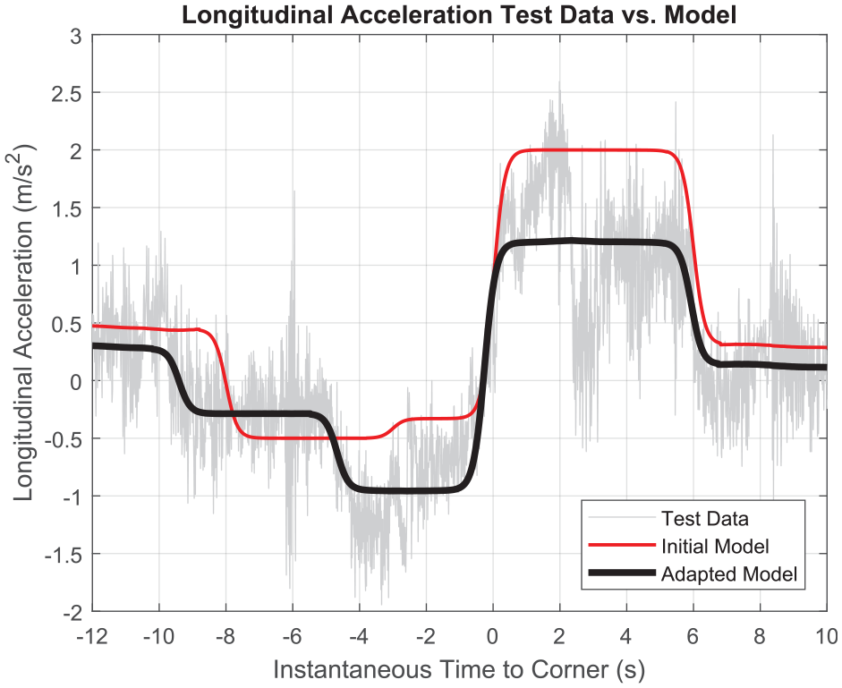
Figure 2 illustrates raw longitudinal acceleration in grey, along with the chosen model in black. Ignoring the red section of the model for now, we can see that the structure of deceleration and acceleration either side of the corner apex at t = 0 s is approximated by a sequence of three specifically timed hyperbolic tan functions. Perfect replication of the deceleration/acceleration sequence is impractical – for example although the driver instigates a distinct deceleration at −5.5 s they decrease the deceleration magnitude in the lead-in to the corner; we can also see a gear-change in the acceleration phase at around +2.5s. By examination of many instances of driver and corner the selected model captures the core components that the driver controls, that is, the acceleration timing, the magnitude of deceleration needed to achieve a comfortable lateral acceleration in the corner, and the subsequent acceleration event. Interestingly we see drivers perform both stages, including the acceleration event, even when corners rapidly follow on from one another, which strongly suggests an open-loop plan of behaviour.
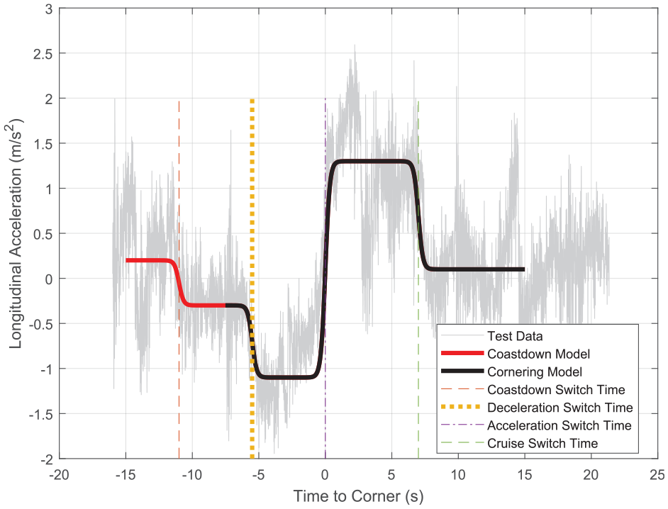
Cornering behaviour acceleration of test data versus model.
Equation (1) describes the pair of deceleration/acceleration actions, illustrated in black in Figure 2:
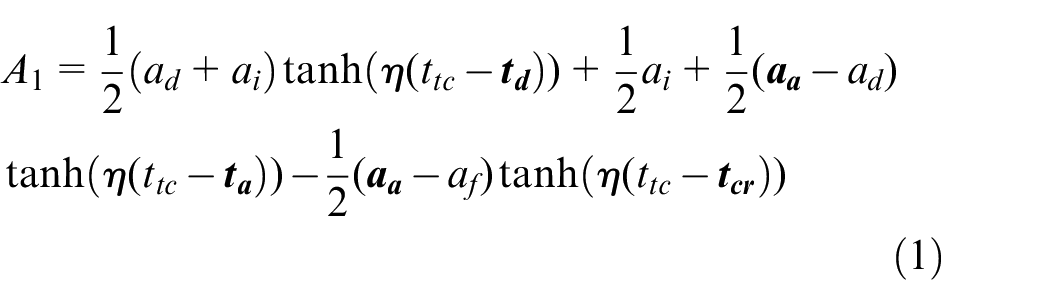
Although apparently complicated, this formulation simply quantifies the timing and magnitudes. The parameter
To give further meaning to the deceleration phase, this is then quantified in terms of the comfortable lateral acceleration magnitude,

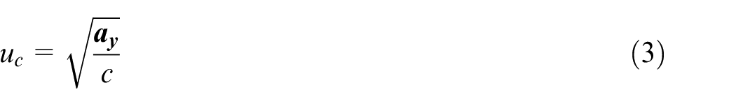
where
Coasting, A2
When approaching a corner that is visible from some distance, most drivers release the acceleration pedal to let the vehicle coast under engine braking before they initiate the core deceleration phase described above. This behaviour is considered a sub-mode of cornering, illustrated by the initial red section of the model in Figure 2, which is modelled in a similar way:
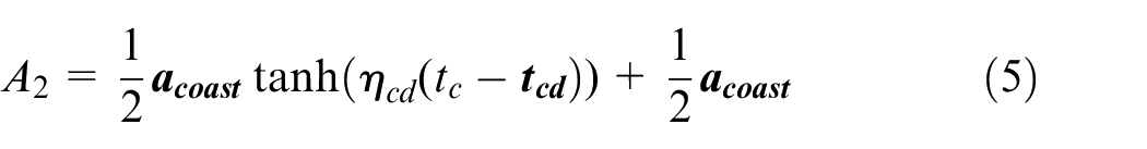
Related to
The parameters
Straight-line speed, A3
Although roads have continuously varying curvature, the known path can easily be divided into discretely identified, ‘significant’ corners, with the remainder of the path below a threshold curvature being considered essentially straight (


This speed varies for each driver and may also vary within the same journey depending on factors such as cognitive load, mood, weather, etc. It is converted to a deviation,

Speed limited behaviour, A4
Driver behaviour for speed limited sections is separated into two stages – approaching the speed limit and driving within the speed limit. The first stage is modelled in the same way as the coasting behaviour,
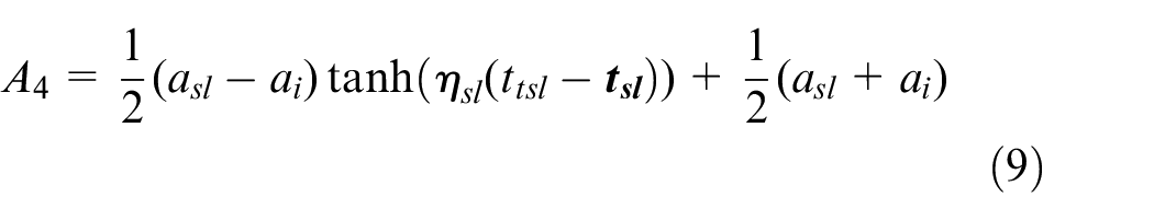
which captures the time to the next speed limit
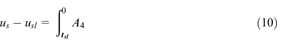
In (9),
The second stage replicates the straight line driving equations (6)–(7), replacing

Model implementation
The open-loop longitudinal controller is applied through the particle model for the appropriate situation

where
The controller logic is provided in full detail with the use of flowcharts in Appendix 2.
Unscented Kalman Filter
Kalman filters are widely used for real-time state estimation of non-linear systems and they can also be applied to identify the parameters of a nonlinear model, for example in Refs.20–22 The adaptation of model parameters can be achieved either alongside or independently from the estimated states, through the use of either an Extended Kalman Filter (EKF) or an Unscented Kalman Filter (UKF). Actually, Ma et al. 17 concludes that either filter can identify parameters equally effectively; the UKF is preferred over EKF here as it eliminates the need for computing system Jacobians. Of course other techniques (such as Bayesian filtering) could be used to optimise the parameter values, and they are likely to function equally well for system identification; the preference for the Kalman filter here comes from its flexibility to be used both in real-time and for identification, in a computationally efficient way.
The definition of the UKF depends on a nonlinear system model,


The magnitude of the errors is represented through covariances


A step by step process of implementing the UKF has been presented by Best.
20
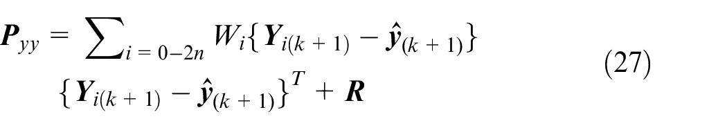
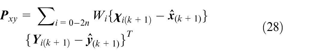
The UKF computes state estimates

This is done using a ‘cloud’ of


where
Using Euler integration, the sigma points are propagated by:

and intermediate estimates for the propagated state and state error covariance matrix are computed by weighted averages as
with
Weighted estimates of the outputs are then obtained from the output model:

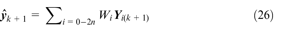
The UKF propagates output error covariance,


Adapting for parameter estimation
With minor modifications to the process described above, the UKF can be modified to enable parameter estimation in addition to, or indeed in place of, state estimation. In this case we can simply define the state vector as the set of parameters of the longitudinal model:
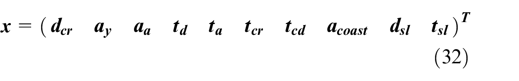
And since there are no actual states in the parameter set, and over any reasonably small time period we would expect parameters to remain constant, the filter’s model for these will be zero:

By doing this, we reduce (14) and (16) to a simplified form that excludes process error altogether.
The sensor outputs are longitudinal velocity and longitudinal acceleration, as measured from the vehicle CAN. Both kinematics are included so that the filter can be driven by single time-step variations in speed (a sensor with a low noise to signal ratio) as well as approximation of the measured acceleration (which has a high noise to signal ratio, as illustrated in Figure 2). By including the Euler integration within the model we eliminate the need to include any input in the state vector; this simplifies the filter and also defines the model as a process to approximate parameters to fit u as a sensor value only. There are two separate modes – for cornering:


And for a derestricted/speed-limited straight line:


Since there are no variable states, the definition of

Furthermore, the filter is able to calculate its own measurement error covariance,


It should also be noted that, due to the propagation of sigma points, the computational load of a UKF increases as 2n with the number n of estimated states (in this case parameters). For ease of nomenclature we pose the UKF here as one single filter with 10 states. However, as the acceleration model varies according to the path topography, it would be straightforward to instead design separate UKF filters for each stage of the model, and switch between them, running only one at any given time. Further, the limited interdependence of parameters would allow the maximum number of parameters for any one of these UKF to be as low as two, which significantly reduces processing requirements.
System identification
The UKF can be used in conjunction with the Longitudinal Model as a real-time process, to continuously capture variations in driver behaviour. As it runs, the error between the sensor set and the model is minimised, thus driving the parameters that govern the shape of the acceleration curve to values that match the sensor more accurately. The single parameter λ can be adjusted to alter the speed of parameter adaptation.
It can also be used as a system identification process to identify the average behaviour for each driver; this is achieved by setting λ to a low value (here λ = 10−7) and running the UKF for each driver over a set of their data repeatedly. This is illustrated for a single driver – corner combination in Figure 3, where the parameters were initialising at nominal sub-optimal values and adapted to the final values as shown in Table 1.
UKF system identification for a single corner.
Initial and final cornering related parameter values.
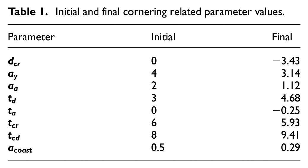
It is important to note that every driver will behave differently over a corner and individual acceleration curves will vary slightly from the model. For example, the portion past the corner apex includes a gear change, with a large momentary drop in acceleration, but the model still manages to capture the overall acceleration impulse and timing. The same is valid for the section before the corner, where the system identification process was purposefully initialised with a value for
Figure 4 shows identification results for the same corner for several drivers. It is clear that each takes an individual approach, with some coasting significantly earlier than others, such as drivers T and W, or accelerating more gently over longer periods – drivers H and X. Driver E also stands out as a driver who decelerates late and hard into the corner.
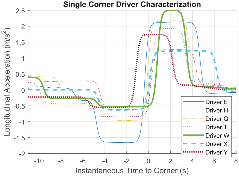
UKF system identification for a single corner for multiple drivers.
When the identification is conducted over a longer section of road, the cornering parameters will not exactly match each individual corner; that is, drivers do not decelerate at exactly the same time with exactly the same magnitude before a corner every time. However, this variation is mitigated to some extent by parameter
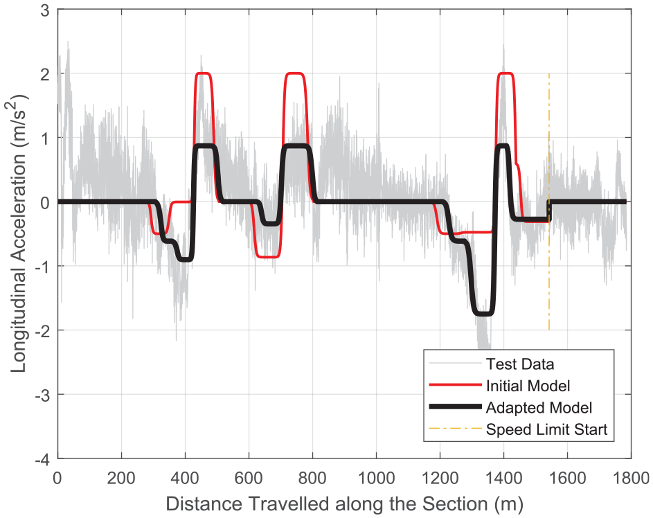
UKF System Identification Acceleration over a Full Section DRIVER G.
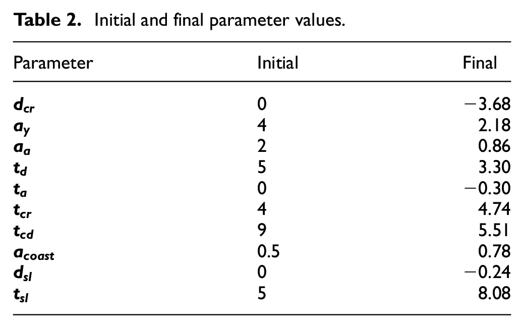
The non-cornering related parameters associated with straight-line driving and speed limit behaviour are also adapted accurately to each individual. The average straight-line derestricted cruise section in Figure 6 on the left from 800 to 1190 m matches the actual cruise speed. This is further illustrated by another section traversed by the same driver with a longer straight-line section –Figure 6 (right) with initial and final parameter values shown in Table 2. The restricted section on the left of 8.2 from 1540 m. onwards also shows the correct adaptation of speed limit deviation for that driver.
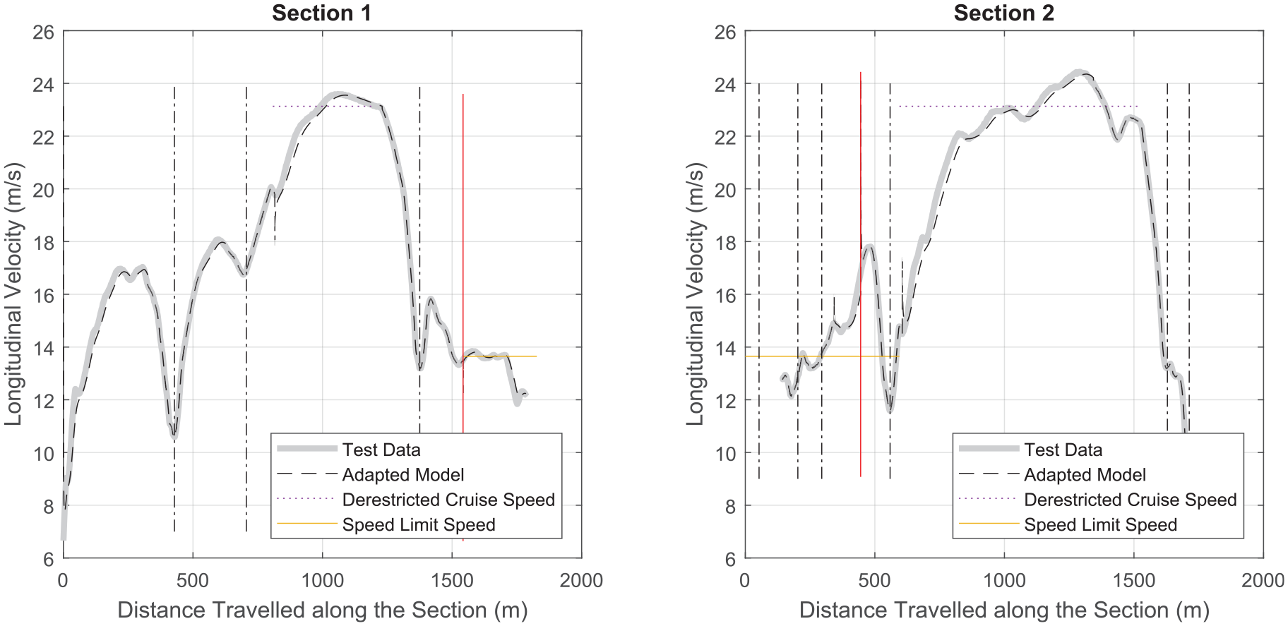
UKF system identification velocity over a full section DRIVER G.
Initial and final parameter values.
Finally, the system identification was conducted on all sections that each driver traversed over a 90 min drive, to find values that are representative of the overall average behaviour of that driver on that day. Figure 7 demonstrates the parameter convergence for this, deliberately slow identification process.
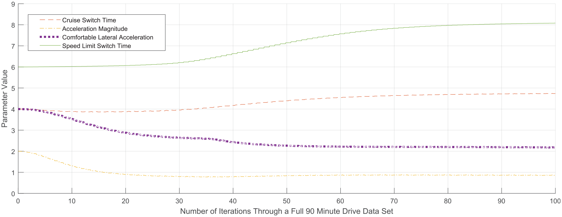
Parameter convergence throughout system identification.
The final mean values of each parameter for each driver found from the last iteration of the identification process defines the characterisation of that driver (on that day) and are shown in Figure 8. These results present a wide spread of behaviour and some interesting observations in the extremes. For example, driver E is consistently late to react to road features such as corners and speed limits as is evident from his low values for
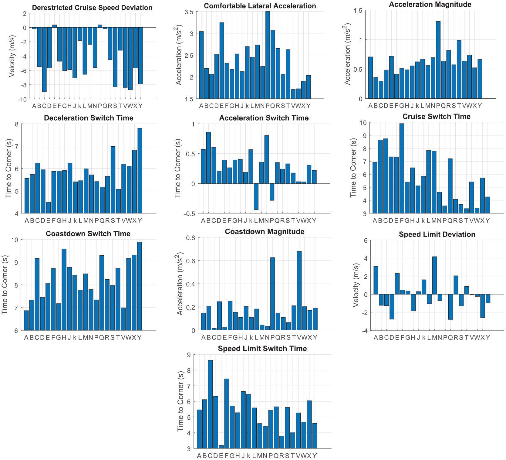
System identification final parameter values.
It is also curious to note that only two drivers – L and P – consistently accelerate ahead of the corner apex, which is also indicative of a dynamic driver. Furthermore, driver P also maintains the fastest average cruise speed.
At the other end of the spectrum, driver Y shows a relaxed style, with a low derestricted cruise speed and lateral acceleration tolerance, who also coasts down and decelerates earlier than the rest of the sample. The whole sample presents a good mix of behaviours in non-extreme parts of the spectrum with substantial variations in each of the parameters suggesting that individual characteristics of each driver are captured. There does not seem to be a strong or simple correlation with age in any of the parameters, though it is interesting that those over 70 (V-Y) all have a preference for low lateral acceleration through corners.
Mapping over-arching driver metrics
Finally, we explore the ability of an identified set of parameters to explain a single overall indicator of driver behaviour, such as their skill, safety, or fuel efficiency. Such ‘global’ metrics are hard to define, but sensible choices can be made in a number of logical ways. Fuel efficiency is easily and directly quantified since engine speed and torque can be used to calculate the total energy used by each driver. Other indicators, such as ‘skill’ and ‘safety’ are much harder to objectively quantify, but inferences can be made to relate more abstract concepts to measurable values. For example, the fuel efficiency of each driver might also be expected to correlate well with how aggressively they drive.
In addition to fuel efficiency, here we will consider a metric for safety by measuring driver speed on a particularly narrow, straight section of road where peripheral vision is obscured by trees and hedges, as shown in Figure 9.
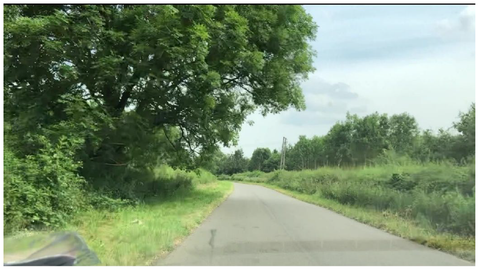
Depiction of an obscured narrow road.
At this point on the road, the driver is not close enough to the upcoming corner to be directly influenced by it, so their speed simply represents the overall level of risk they are willing to take while driving on a straight but narrow road. We do not claim this to be a sophisticated or complete metric for safety – it is just used as an indicator; other more complex objective measurements could be used. The purpose is to demonstrate the ability of the information in the driver parameters to model other appropriately separate metrics.
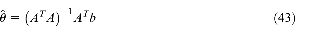
As we have a relatively large number of parameters (10) to map the metrics of a reasonably small sample of drivers (22) it is statistically prudent to find a reduced subset of parameters for this regression, and also to test the regression model in an independent way. A sub-set of the identified parameters can be used as the regressors in an Ordinary Least Squares (OLS) linear regression,

where, for the right-hand side,
Using all 10 parameters to fit the metric for just 22 drivers presents problems in terms of statistical significance, since noise in the parameters can explain b by chance. The case is only statistically compelling if a relatively small sub-set of parameters achieves a good fit.
A method of Singular Value Decomposition (SVD) presented in Tuplin 24 can be used to find the rank of significance of parameters. First, b and each of the 10 columns of the full candidate set of A is normalised by removing the mean and dividing by the vector norm. The single parameter that will have the greatest contribution to explain b can then be obtained from

We can then define a new

Where U and V are orthonormal rotation matrices, so the equation can be rewritten:

with
In the first iteration,

where
Figure 10 shows the corresponding model error (|
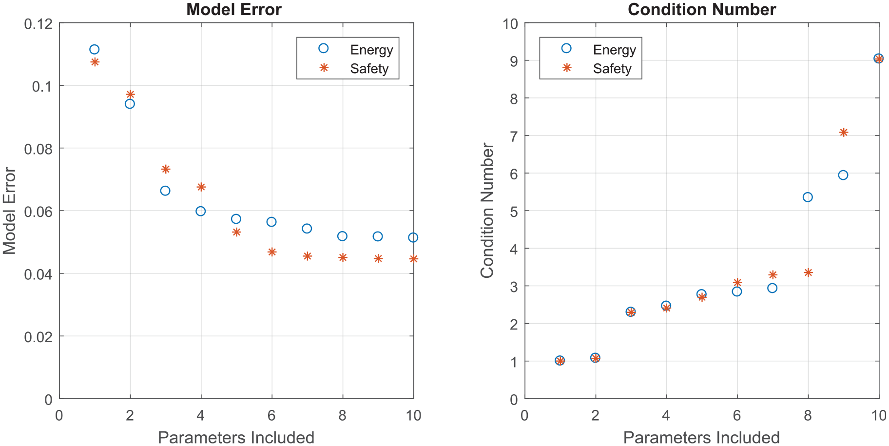
Model error and condition number for an increasing set of parameters in the fit.
It is immediately clear that a subset of just five factors for the safety metric provides model errors that are almost as low as for 10 factors, together with good conditioning. It is less clear whether a subset of three or seven parameters is appropriate for the energy metric. It is therefore interesting to also consider the rank order of significance of the parameters, which is shown in Table 3 for both indicators.
Parameter order of significance for both indicators (1 being the most significant parameter in the regression).
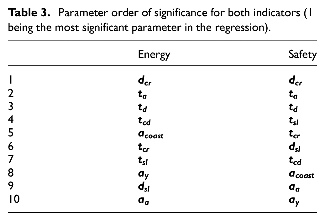
In both models, the most significant parameters are
For the energy model, the next two parameters pertain to coastdown behaviour. This makes sense as more gradual velocity changes use less energy. Following that are the remaining temporal parameters. The ranking of
For the safety model, it is interesting that the temporal parameters are of greatest significance. With regards to
To test the efficacy of the final three factor energy and five-factor safety models in an unbiased way, a validation is run by excluding a driver from the fitting process and examining the result obtained when the model
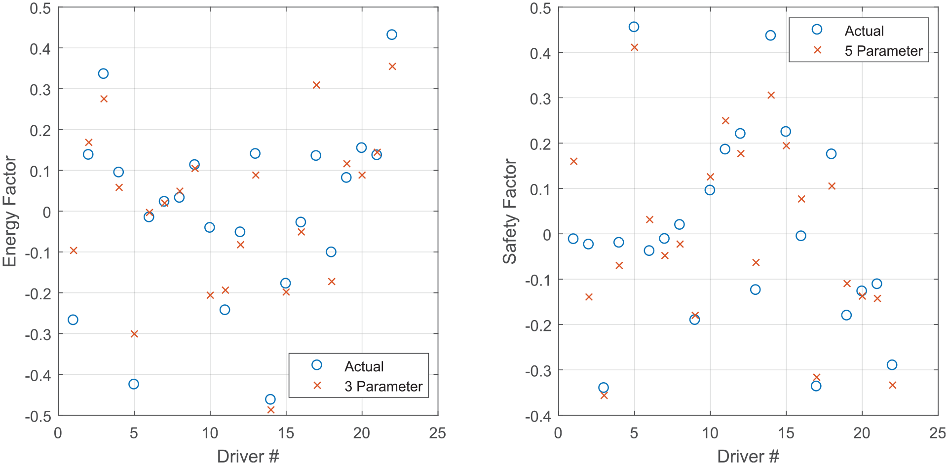
Model accuracy comparison for driver excluded from the fit.
Although not perfect for all drivers, in most cases the model fit is very good; this method is certainly reliable for deciding broadly whether a given driver is energy wasteful or not, and what broad range of ‘safety factor’ they have, from only the most significant adapted characterisation parameters.
Conclusion
This paper presents a means of fully characterising a driver in terms of a set of parameters that are estimated by a UKF used in combination with a dynamic model. Although at this stage the model has been tested using only one driving scenario, the structure could easily be expanded to other free-driving conditions.
By adopting an open-loop acceleration structure, the model captures routine, pre-planned aspects of driving which most readily characterise driving style. A significant novelty is in the estimation of time-based parameters, which turn out to be important indicators of driver behaviour when the model is correlated to other factors, such as energy wastefulness and a measure of safety.
The filter can operate in real-time using readily-available longitudinal velocity and acceleration signals; it is thus capable of capturing variations in driving behaviour caused by change of mood or other journey-specific conditions. The full characterisation has also been correlated against additional metrics of energy wastefulness and a safety factor. Although the safety factor can not be considered in any way comprehensive, both metrics are suitably independent from the driver model parameters themselves. The ability of a relatively small sub-set of model parameters to map both metrics demonstrates that they appropriately span the behaviour range of the drivers included in the study.
Further development of this work will incorporate the steering model developed in Banerjee et al. 13 to establish a combined lateral-longitudinal driver characterisation, and to consider a wider range of road types.
Footnotes
Appendix 1
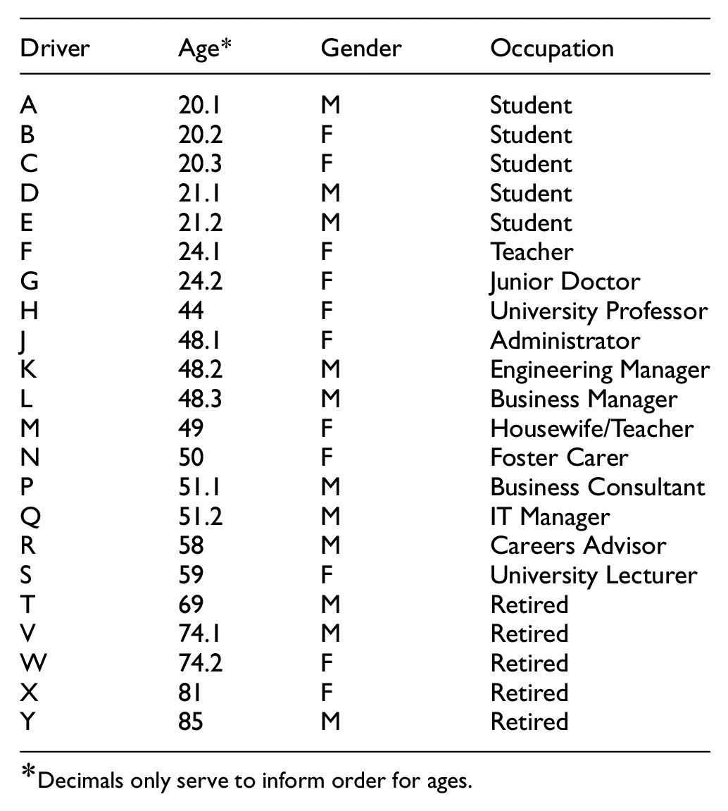
| Driver | Age* | Gender | Occupation |
|---|---|---|---|
| A | 20.1 | M | Student |
| B | 20.2 | F | Student |
| C | 20.3 | F | Student |
| D | 21.1 | M | Student |
| E | 21.2 | M | Student |
| F | 24.1 | F | Teacher |
| G | 24.2 | F | Junior Doctor |
| H | 44 | F | University Professor |
| J | 48.1 | F | Administrator |
| K | 48.2 | M | Engineering Manager |
| L | 48.3 | M | Business Manager |
| M | 49 | F | Housewife/Teacher |
| N | 50 | F | Foster Carer |
| P | 51.1 | M | Business Consultant |
| Q | 51.2 | M | IT Manager |
| R | 58 | M | Careers Advisor |
| S | 59 | F | University Lecturer |
| T | 69 | M | Retired |
| V | 74.1 | M | Retired |
| W | 74.2 | F | Retired |
| X | 81 | F | Retired |
| Y | 85 | M | Retired |
Decimals only serve to inform order for ages.
Appendix 2
The controller logic is displayed in the flowcharts in Figures A–C. It relies on setting specific flags for corner, speed limit and coastdown behaviour and indices for relevant corners and speed limits. The flowchart has been split up into three significant blocks – one that governs which mode of behaviour should be relevant and two that govern index advancement and flag setting for both speed limits and corners.
Additional conditions are as shown below to make sure the vehicle is not on the approach to a speed limit, is also past the corner apex but is before cruise behaviour to address a niche scenario so that speed limit approach behaviour takes precedence over corner behaviour:
Early corner and speed limit approach provision – in Figures 5 and 6 refers to the special situation where the vehicle is past the current corner apex and either approaching the next corner sooner than expected or approaching a speed limit:
In both cases, where the corner index is being increased in Figures 5 and 6, we will check that the next upcoming corner is at least 10 s further away than the current coastdown switch time:
Declaration of conflicting interests
The author(s) declared no potential conflicts of interest with respect to the research, authorship, and/or publication of this article.
Funding
The author(s) received no financial support for the research, authorship, and/or publication of this article.