
Abstract
The physical modeling-based approaches tend to be over-simplistic and cannot forecast the complex dynamical phenomena, thus leading to non-negligible errors. It is not easy to measure some parameters precisely, and they are usually approximated roughly. However, this approximation reduces the modeling accuracy of the physical model, which is a common problem in complex systems research. It is well-known that neural networks are capable of encoding dynamic information. The vehicle can be accurately modeled by collecting data during its motion. However, purely data-driven approaches have low interpretability and cannot be used in commercial applications. In this work, we present a new hybrid modeling architecture. Based on the physical model, the deep learning method is introduced to expand the incomplete dynamics described by differential equations. Compared with the physical modeling-based and purely data-driven approaches, the proposed technique has lower modeling error and higher interpretability. We evaluate the performance of the hybrid model based on the collected data. The test results show that the proposed architecture successfully captures the vehicle dynamics and reduces the error caused by multi-step prediction compared to the data-driven models. The results also show that the proposed method has value for significant research and practical application.
Introduction
Autonomy is the future of automobile development. Autonomous vehicles are considerably transforming the ecology and travel modes. The classic self-driving systems typically include perception, positioning, decision making, trajectory planning, and control module. Accurate kinetic information of the vehicle ensures the safety of autonomous vehicles.
In the last century, physical modeling-based approaches have been widely studied. In the mid-20th century, researchers from Cornell University studied the linear two degrees of freedom vehicle model. 1 The researchers assumed the whole vehicle is a rigid body and considered the cornering stiffness of the front and rear axles. In addition, the authors did not distinguish between the wheels on the left and right sides. The wheel angle is directly used as the input of the model, and the understeer and oversteer characteristics of the car are defined. Segel 2 regarded the vehicle as a linear dynamical system and established a three-DOF vehicle model including yaw, lateral, and roll motions to describe the steering response. Kazemi et al. 3 established a non-linear 7-DOF vehicle model using the magic formula tire model and studied the influence of the rear-wheel steering on the vehicle’s stability during driving. Notably, the parameters of these models have actual physical meanings. Therefore, they have high interpretability. However, the physical model based on the first principles is usually idealized during modeling. Consequently, it is impossible to accurately calculate the true dynamic response of the vehicle during experimental driving, such as the front and rear axles of the vehicle load transfer and the high-order dynamic response of tires. Generally, the environment in which the physical model tests are performed is different from the actual environment, thus making it difficult to estimate the model parameters in real-time.
With the development of deep learning, significant progress has been made in many research fields, especially in autonomous driving. The deep learning-based methods have been successfully used to perform perceptual tasks, such as target detection,4–8 image segmentation,9–11 and trajectory prediction. 12 Recently, various works have been proposed that use deep learning in an end-to-end fashion to control the vehicles based on the original sensor data.13,14 These methods directly obtain the instructions at the output end from the image information at the input end. It is noteworthy that neural network training requires a large amount of data. The neural networks have strong nonlinear modeling capabilities. The authors 15 proved that the nonlinear modeling ability of a neural network could be combined with the feedback, and the input and output data of the system can be used to model the nonlinear systems accurately. Ji et al. 16 proposed an adaptive control mechanism based on the Lyapunov stability theory and radial basis function neural network (RBFNN). This network uses an ANN to estimate the uncertainty in tire cornering stiffness. Spielberg et al. 17 established a vehicle lateral dynamics model based on a neural network and successfully used it to design a trajectory tracking controller. Simon et al. 18 studied and optimized a neural network’s size, structure, and initial weights for modeling. In addition, the authors also examine the results of the fusion weight network. Kabzan et al. 19 established a data-driven and mechanism mixed model using a relatively simple and nominal model. The researchers also established the online learning of model error based on Gaussian process regression. Compared with physical models, the dynamic models based on neural networks require almost no specific domain knowledge. In addition, the construction cost of the model is high as the network parameters are learned using a large amount of data. Although the data-driven model can be changed according to the continuous changes in the environment, it is difficult to solve the model parameter estimation due to using a nonlinear algorithm. However, the interpretability of the neural network is low as the weight parameters of the network cannot correspond to the parameters of the physical model. In addition, the data-driven model is prone to cause uncontrollable errors compared with the traditional physical model, which reduces the safety of the autonomous vehicle during driving. In case of an error message inside the neural network, it is impossible to locate the source of the error message.
When using neural networks to model dynamic systems, the network’s convergence speed and prediction accuracy can be improved by incorporating prior knowledge. In system identification, the white-box model is one of the most convenient methods to represent prior knowledge. However, because the white-box model is simplified and assumed to be unable to capture too many complex nonlinearities acting on the system, its output error is considerably high. One way to solve these shortcomings is to combine an analysis model with a neural network to improve the overall performance. For the time series prediction task, researchers have proved that the performance of the hybrid model is better than that of the analysis model and artificial neural network.20,21 Furthermore, the existing methods have shown the potential of a hybrid neural network model in dynamic system modeling. Jiahao et al. 22 have demonstrated neural networks’ compatibility with first-principle dynamic models by modeling various nonlinear systems. Chee et al. 23 used a deep learning method and differential equations to augment a model obtained from first principles. Holzmann et al. 24 used the radial basis function network to compensate for the influences of changing road conditions affecting a vehicle dynamics simulation model. Pracny et al. 25 coupled neural networks and spline function to study the influence of oil temperature change on the operating characteristics of the shock absorber. Fraikin et al. 26 established an efficient and accurate vehicle lateral dynamics simulation by coupling the long short-term memory (LSTM) neural network with the single-track model. Graeber et al. 27 combined neural networks with a vehicle kinematics model in the side-slip angle estimation and increased the number of input features of a neural network by using the kinematics model to improve the estimation quality of the side-slip angle. Mohajerin et al. 28 combined the proposed RNN-based black-box models with a physics-based into a single RNN-based modeling system, solving many of the limitations of the existing state-of-the-art in long-term prediction for dynamic systems. However, the neural network’s output is used as the input of the physical model, which may cause the input-output relationship of the physical model to be obscured by the neural network. De Groote et al. 29 proposed a neural network-enhanced physical model for modeling the servo system. The unknown loads and parameters in the physical model are obtained using the neural network. Nevertheless, the final output is obtained from the physical model. Since the modeling method requires high accuracy of the physical model in the hybrid model, it is not suitable for complex dynamic systems, such as vehicle dynamic system. Another challenge is that it is difficult to train hybrid model due to inaccurate physical models. Since the prediction state will be feedback to the input port, the error increases with time, which causes divergence in the weights of the neural networks.
To address these challenges, we propose a new hybrid model for the multi-step prediction of vehicle state. The main contributions of this study are stated as follows.
(1) We employ a hybrid model to develop a high-fidelity vehicle model capable of capturing poorly understood uncertainties and residual dynamics. The hybrid model combines prior knowledge of the system dynamic and better represents the vehicle dynamics.
(2) We show that the hybrid model significantly improves state predictions’ accuracy over the nominal model and a separate data-driven-based prediction model.
(3) To reduce the divergence during the training of the hybrid model in multi-step prediction, we use open-loop and closed-loop training methods so that the inaccurate physical model is used as a part of the hybrid model.
The rest of this paper is structured as follows. In Section II, the overall architecture and composition of the hybrid model used for multi-step prediction are presented. In Section ãÂ, the vehicle dynamics data collection and model training methods are introduced. In Section ãÈ, the predictive performance of physical models, neural network, and hybrid models are evaluated. We conclude this work in Section ãÈ.
Hybrid model for multi-step prediction
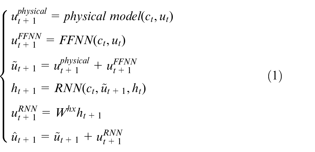
In this section, we present the framework and methodology of the hybrid model. The proposed algorithm is mainly composed of three components: the physical model, feed-forward neural network (FFNN), and recurrent neural network (RNN).
The structure of hybrid model
Figure 1 shows our suggested hybrid model, comprising three modules: a physical model, a FFNN and an RNN (with initialization networks). The physical model receives current
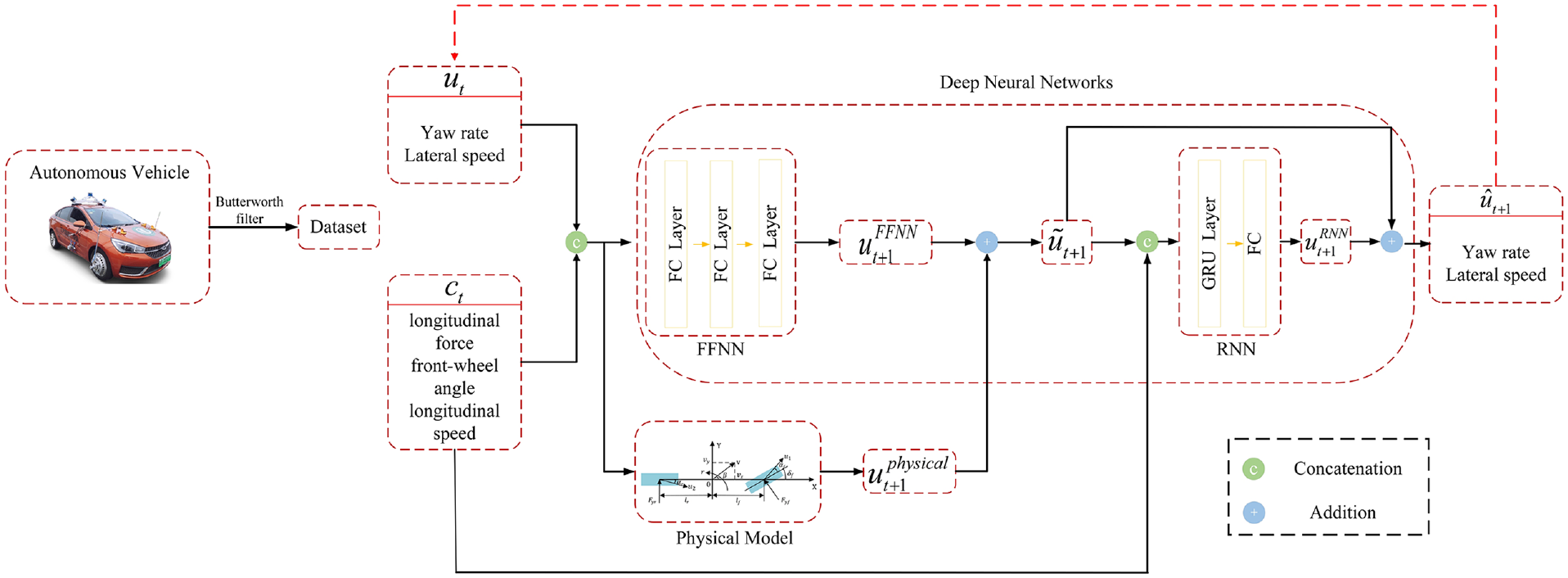
The proposed hybrid architecture consists of a physical model, FFNN, and RNN.
During the process of multi-step prediction, the feedback loop indicated by the red arrow provides feedback of the previous state to the input for predicting the next state. Due to an increase in the feedback, the multi-step prediction error accumulates over time. In this work, we define
Physical model
The kinematic model and dynamics models are commonly used in vehicle motion simulation. The kinematic model uses the kinematic correlation to describe the motion of an object in space. The dynamic model can be established by describing the forces acting on an object. In this section, the vehicle dynamic model used for hybrid modeling of vehicle lateral dynamics are described, including single-track model and brush Fiala model.
The self-driving cars run on a flat road and the factors, such as the slope and the vertical movement, are ignored.
The suspension system and vehicle are rigid. The influence of suspension motion and its coupling are ignored.
Only the tire cornering characteristics are considered. The relationship between the longitudinal coupling of the tire forces is ignored.
A 2-DOF vehicle model is used to describe the movement of the vehicle without considering the left and right load transfer.
The longitudinal speed of the vehicle is constant and the weight transfer of the front and rear axles is ignored.
The resistance, such as vertical and horizontal aerodynamics, is also ignored.
In Figure 2,
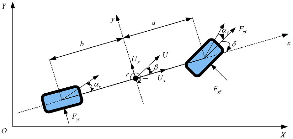
The schematic of a single-track model.
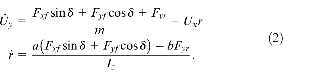
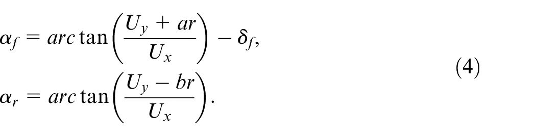
The dynamics single-track model is expressed as follows:
The nonlinear characteristics of a vehicle during driving under different road conditions arise from the tires, when the vehicle is turning. Therefore, in order to expand the scope of application of a vehicle model, a nonlinear tire model is introduced as follows. The tire lateral force is respectively calculated as:
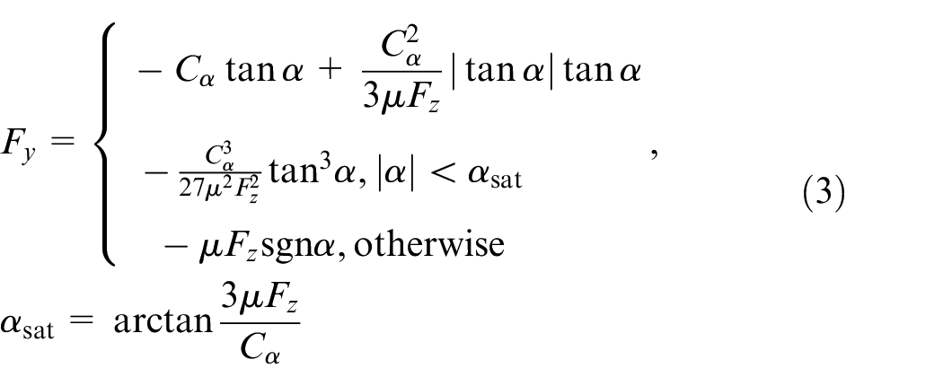
where,
When the vehicle’s longitudinal speed changes slowly, the load transfer between the front and rear axles can be ignored. The amount of normal force experienced on each tire is respectively calculated by:
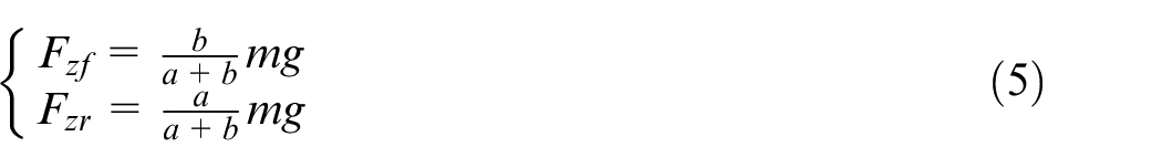
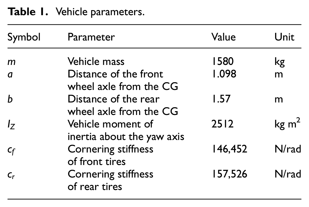
The real vehicle parameters corresponding to the simplified vehicle dynamics model are shown in Table 1.
Vehicle parameters.
Feed-forward neural networks
Hornik et al. 30 proved that a FFNN with a hidden layer could approximate any continuous function. It has been used extensively in the modeling and control of dynamic systems and as the modeling part of the controller in the Lyapunov design method to stabilize the system. 31 Since FFNN cannot capture the long-term characteristics of a dynamic system, it is mainly used to capture poorly understood uncertainties and residual dynamics. In this work, FFNN comprises three fully connected layers and ReLU activation functions as a single-step predictor or compensator.
Recurrent neural networks
In this section, we present the basic concepts of RNN and gated recurrent unit (GRU). The RNN has proved their advantages in time sequence modeling, such as natural language processing and trajectory prediction. These networks have proved to be more effective than the traditional networks for modeling long-term dependence between the current and historical information. We present a vanilla RNN and use a GRU to enhance its performance. A schematic structure of the RNN is shown in Figure 3.
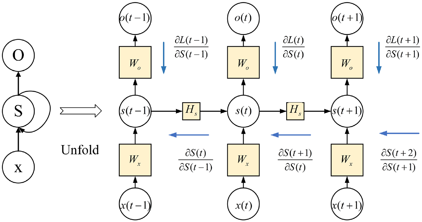
The schematic structure of RNN.
The RNN is mathematically expressed as:


where
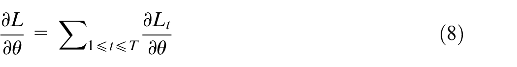
The blue arrow in Figure 3 indicates the chain-rule-based Back Propagation Through Time (BPTT) scheme, which is expressed as:
where,
Gate recurrent units
Unlike FFNN, RNN can take sequences of arbitrary length as input. It has the property of universal approximation and can reconstruct the state space of a dynamical system well in theory, enabling suitable models for multi-step prediction problems. Jin et al. 32 showed that RNN might be used to approximate uniformly a state-space trajectory produced by a discrete-time nonlinear system. Due to the large delay between vehicle response and driver input, RNN will offer good performance. Sepp et al. 33 proposed an LSTM model, which improves the long-term modeling ability and has been widely used for participants’ trajectory predictions. However, due to many model parameters, the LSTM model takes longer to process large datasets. Cho et al. 34 proposed GRU. The GRU simplifies the structure of LSTM, reduces the number of gates, and improves operational efficiency.
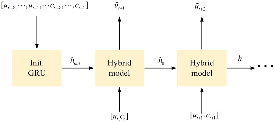
RNN state initialization
The multi-step prediction models, such as LSTMs and GRUs, rely on accurate hidden states to produce accurate predictions. The initial state of the GRU should contain historical information. Mohajerin and Waslander 35 described different LSTM hidden state initializations in the quadrotor modeling using RNN. The authors finally used another layer of LSTM as the initializer. An initialization network extracts the potential dynamics from the historical data. Please note that using the final hidden state of the initializer to initialize the predictive network improves the long-term prediction performance of a network. In this work, we choose another layer of GRU to receive the historical data to generate the hidden states of the predictive network (Figure 4), which are expressed as:

The schematic structure of GRU cells and regression layers.
where,
Experiments and dataset
Data collection and processing
We collected the trajectory samples based on the “Chery Arezer 5E” for approximately 48 min. The dataset includes the dynamic response data of an intelligent vehicle under dry and wet road conditions. The test platform is presented in Figure 5. This platform includes an environment sensing system, inertial navigation and positioning system, a decision control module, and an underlying actuator by wire. The wheel force sensors, S-Motion DTI, and MSW DTI sensors are also installed.
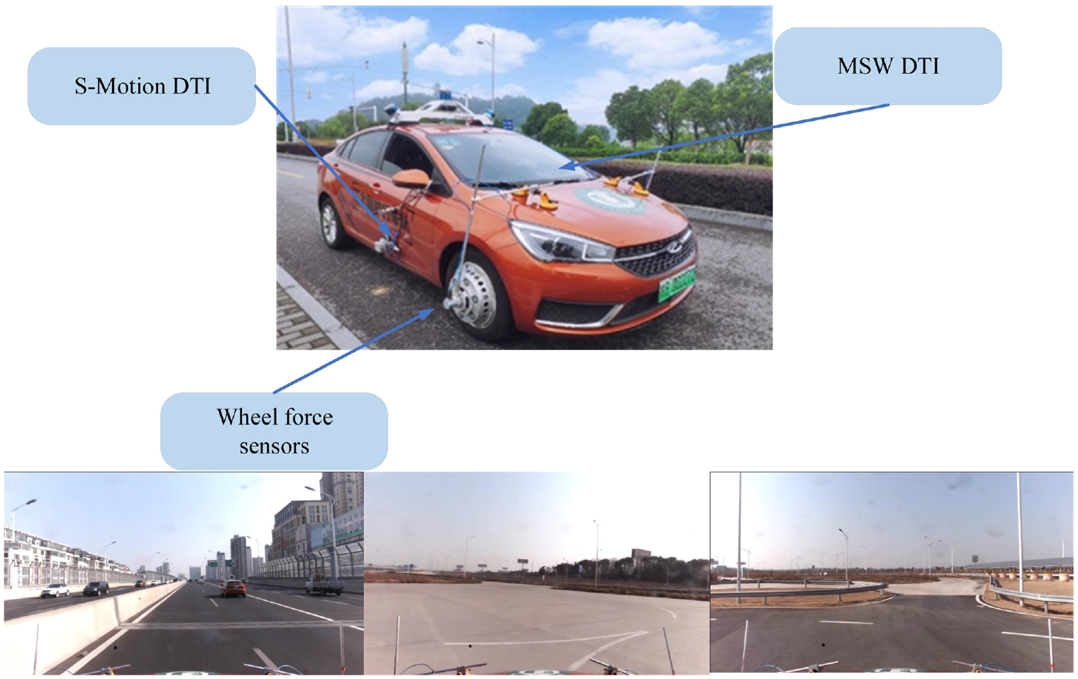
The intelligent driving platform used in this work.
During data collection, the sampling frequency of the signal is 10 kHz. However, there is noise interference in the accumulated data. We use a mean filter to down-sample the collected data to 100 Hz to reduce the training complexity. A second-order Butterworth low-pass filter with a cut-off frequency of 2 Hz is used for data smoothing and filtering out the impact of high-frequency behaviors, such as suspension vibration on vehicle dynamics. The data filtering is completed using an Intel Core i7 2.5 GH computer and MATLAB 2020a. Though the friction coefficient between the tire and road slightly changes in actual conditions, we assume that the friction coefficient between tire and road is constant. The friction coefficients between the tire and dry road and between the tire and wet road are 0.85 and 0.5, respectively. We use 80% of the data for model training, and 20% of the data is used to test the model.
Training methods
The training of the hybrid model is divided into FFNN training and GRU training. In the first stage, FFNN is used to compensate for the single-step prediction error between the output of the physical model and the actual measured value. The loss function used for training FFNN is expressed as:
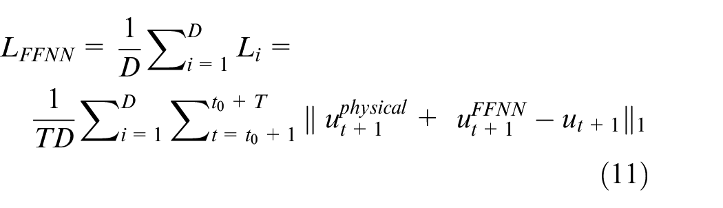
where,
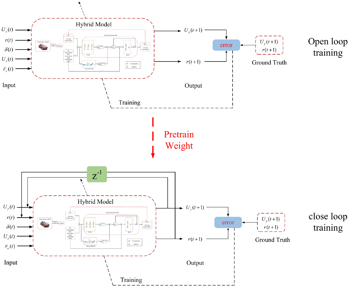
Given the initial state of GRU and the amount of control in the future, the multi-step prediction training of GRU is difficult because the input of FFNN and the physical model depends on the previous inaccurate output. The error accumulates in multiple time steps and finally leads to divergence between the predicted state and the real state. As GRU uses the BPTT algorithm for backpropagation and updating parameters, it is more sensitive to errors. The error accumulation leads to gradient explosion, thus making GRU difficult to train. We use open-loop and closed-loop training to address this problem (Figure 6).
Open loop and close loop training process.
Open-loop training: In open-loop training, we use the pre-training weights of FFNN to train the hybrid model. The teacher forcing is used as the training method.
36
The physical model and FFNN accept the true prior state as input at the time step
Closed-loop training: In the closed-loop training phase, the hybrid model learns to predict the states over multiple time steps without receiving the true states as input. This is achieved by using the state prediction from the previous time step as the input to the current prediction step. The training is still effective because the open-loop training phase ensures that the hybrid model achieves sufficiently accurate predictions to prevent strong divergence of the GRU gradient. In closed-loop training, the pre-training weights during the open-loop training are used to continue training.
The loss function used in open-loop training phase is expressed as follows:


where,
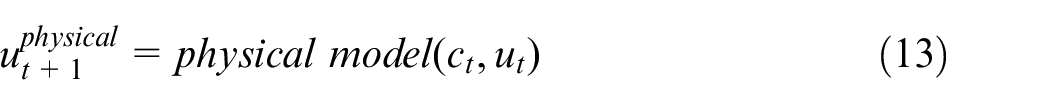
The model does not accept the true input in the closed-loop training phase, and rather, it accepts the output of the previous time step as the input of the next time step. The input of the physical model and FFNN change in the closed-loop training:


Experimental setup
The Facebook PyTorch package in Python 3.6 is used for implementing and training the networks. In the FFNN training phase, we set the learning rate to 0.0001 and mini-batch to 500. In the GRU training phase, we use the exponential decay learning rate to train the model. The initial learning rate is set to

The optimization is performed by using the standard ADAM optimizer. 37 In order to avoid the gradient explosion during the training process, we set the maximum threshold of gradient change to 10 and minibatch to 128 when the model parameters are updated in each step.
Model selection
Hyperparameter search is performed via grid search on the test dataset where prediction time steps T = 0.5 s. The initial network, FFNN and RNN use the same number of hidden neurons. GRU Encoder-Decoder (GRU-ED) is used as a deep neural network baseline. The structure of the hybrid model and GRU-ED are of one hidden layer with the structure chosen as 32, 64, 128, and 256. The best model is chosen based on the root mean sum-of-squared error 35 (RMSSE) on the test dataset. The RMSSE is defined as
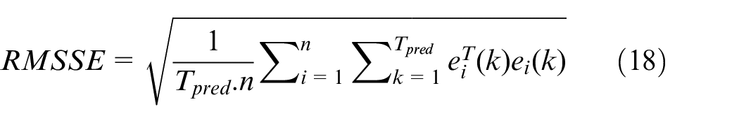
where n is the size of the test dataset, e is the predict error.
As shown in Figure 7, by increasing parameters, the test RMSSE in the hybrid model and GRU-ED significantly reduces, showing that adding model hidden neurons has the ability to significantly reduce prediction error. By adding additional hidden neurons, generally, RMSSE continues to decrease. However, additional parameters increase the size of the model, which increases computational complexity and solves time or causes network overfitting. Ultimately128 hidden neurons are chosen because of their predictive performance and resulting short solve time compared to the large model.
Network size versus RMSSE: (a) RMSSE changes with GRU-ED parameters for high friction data and (b) RMSSE changes with hybrid model parameters for high friction data.
Evaluation metrics
In order to evaluate the prediction accuracy of the model, the mean absolute error and distribution of prediction error in each time step are analyzed. The distribution of error in each time step is represented by using boxplots. The mean absolute error in each time step is evaluated by the L1 norm:
where,
Result and discussion
In this section, the hybrid model prediction performance is compared with both the white-box and black-box models. It is demonstrated that the hybrid models provide a more accurate and reliable prediction than the white-box and black-box models.
Hybrid model versus physical model
Due to simplifying the parameters of the physical model, it is not suitable for multi-step prediction. The performances of the one-step prediction of the hybrid model and the physical model are compared in Figure 8. The results show that the hybrid model’s performance is better than the physical model. Compared with the hybrid model, the physical model has a large deviation.
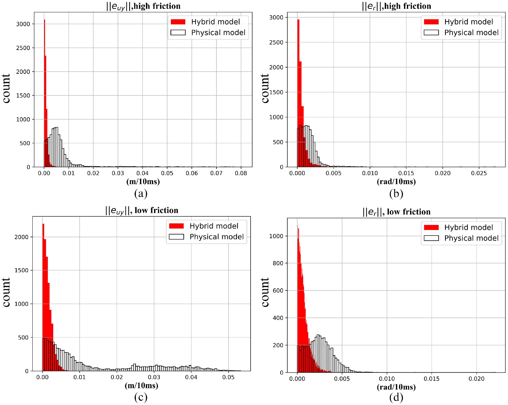
The white-box prediction performance: (a, b) histograms of the lateral velocity and yaw rate single-step prediction errors for the white-box and hybrid model for high friction surface and (c, d) histograms of the lateral velocity and yaw rate single-step prediction errors for the white-box and hybrid model for low friction surface.
Hybrid model versus GRU encoder-decoder
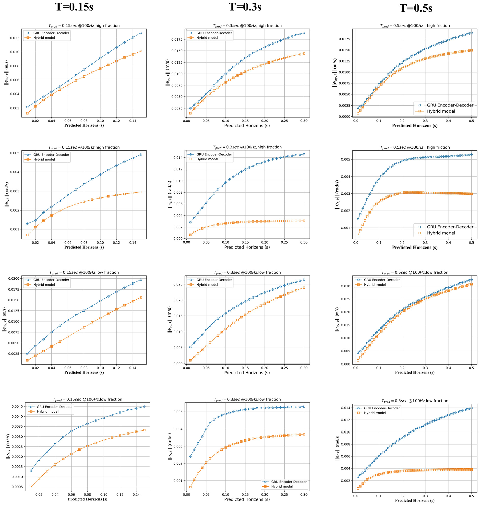
In Figures 9 and 10 and Tables 2–4, the plots and tables illustrate the mean of the test error over the prediction and the evolution of the training cost over the training process. Each column corresponds to one prediction length, which, from left to right, are T = 0.15, 0.3, and 0.5 s. It can be observed that the hybrid model has reduced the prediction error and the training cost significantly. Please note that each model uses the same hyperparameters and is trained for six epochs.
The L1 normal error of lateral velocity and yaw rate, T = 0.15 s.
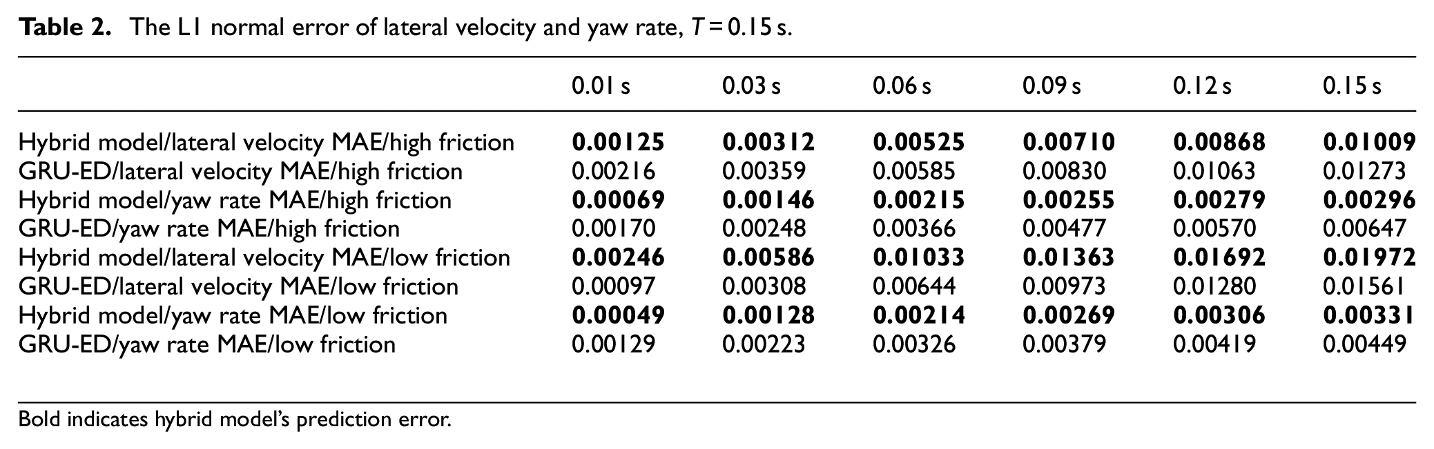
Bold indicates hybrid model’s prediction error.
The L1 normal error of lateral velocity and yaw rate, T = 0.3 s.
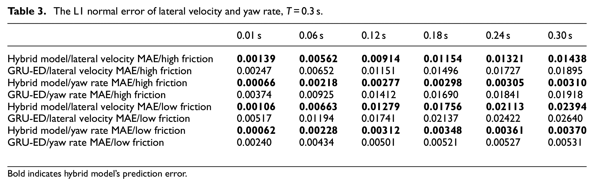
Bold indicates hybrid model’s prediction error.
The L1 normal error of lateral velocity and yaw rate, T = 0.5 s.
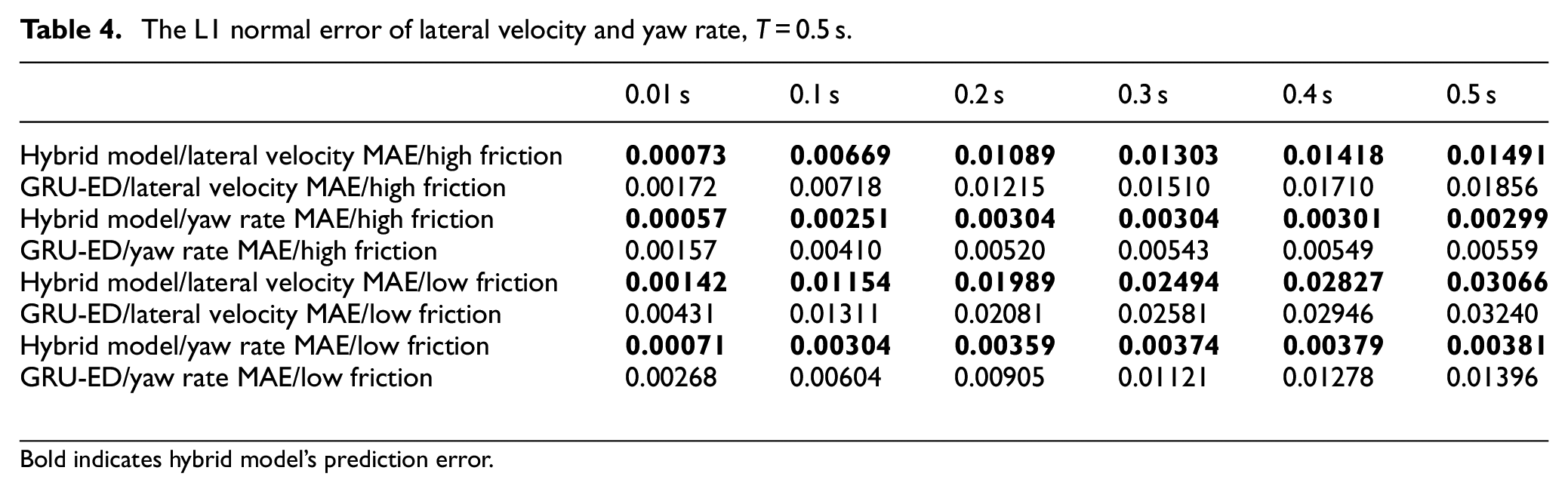
Bold indicates hybrid model’s prediction error.
Comparison between hybrid model and GRU-ED on the vehicle lateral velocity and yaw rate.
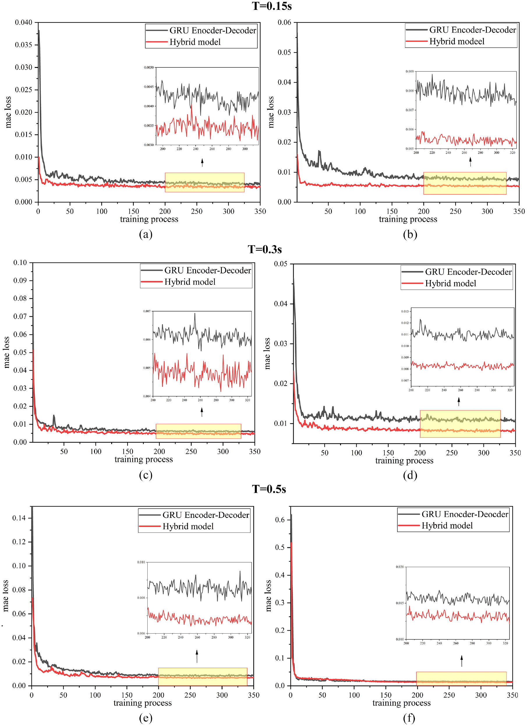
The training performance of the proposed model on the actual vehicle dataset. (From top to bottom = 0.15, 0.3, and 0.5 s. Left column is training process for high friction data. Right column is training process for low friction data.): (a) is case 1 of training process with the prediction time T=0.15s, (b) is case 2 of training process with the prediction time T=0.15s, (c) is case 1 of training process with the prediction time T=0.3s, (d) is case 2 of training process with the prediction time T=0.3s, (e) is case 1 of training process with the prediction time T=0.5s, and (f) is case 2 of training process with the prediction time T=0.5s.
The prediction performance of the model can be further evaluated by studying the error distribution. The lateral velocity and yaw velocity prediction error distributions of the hybrid model and GRU-ED are presented using boxplots in Figures 11 and 12, respectively. In each prediction time step, the yellow dotted line represents the median, the lower and upper limits of the blue rectangle correspond to the upper and lower quartiles q1 and q3, and the ends of the whiskers correspond to extreme cases.
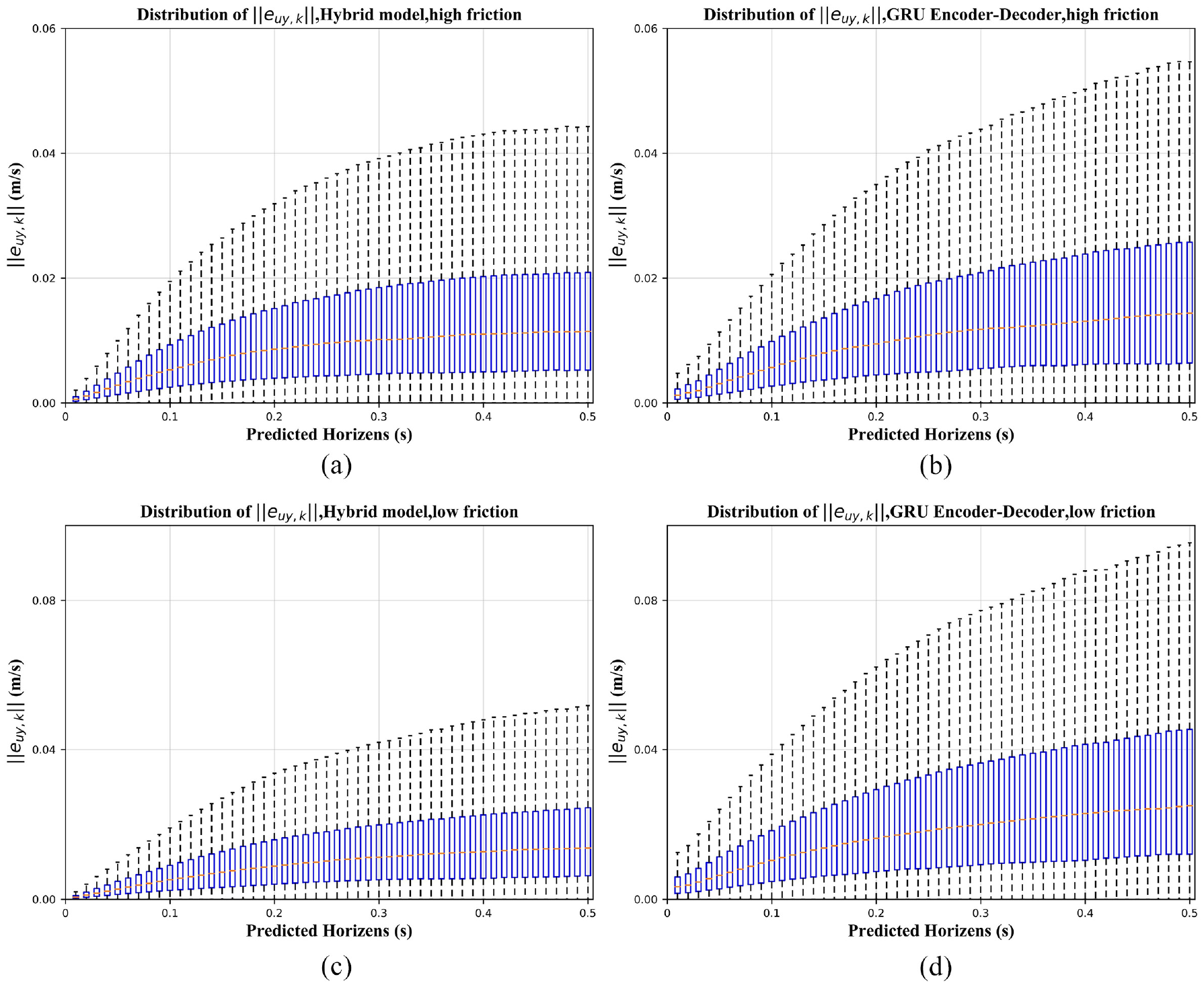
The comparison between the hybrid model and GRU-ED prediction error. The distribution of the L1 norm of the lateral velocity prediction error is plotted for prediction lengths, T = 0.5 s. The plots on the left represent the hybrid model and the plot on the right side represents the GRU-ED: (a) is the prediction error of lateral velocity with hybrid model for high friction data, (b) is the prediction error of lateral velocity with GRU-ED for high friction data, (c) is the prediction error of lateral velocity with hybrid model for low friction data, and (d) is the prediction error of lateral velocity with GRU-ED for low friction data.
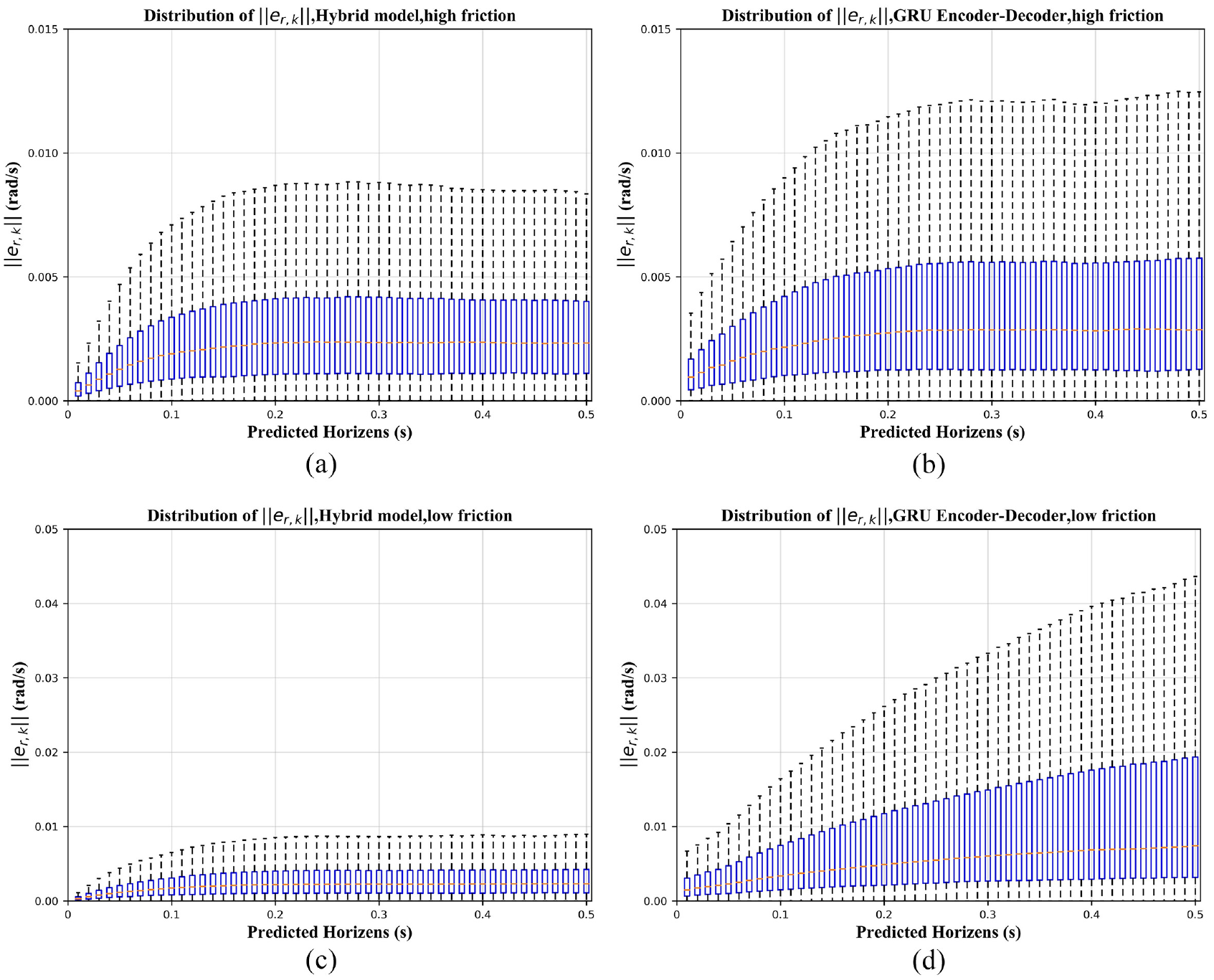
The comparison between the hybrid model and GRU-ED prediction error. The distribution of the L1 norm of the yaw rate prediction error is plotted for prediction lengths, T = 0.5 s. The plots on the left represent the hybrid model and the plots on right represent the GRU-ED: (a) is the prediction error of yaw rate with hybrid model for high friction data, (b) is the prediction error of yaw rate with GRU-ED for high friction data, (c) is the prediction error of yaw rate with hybrid model for low friction data, and (d) is the prediction error of yaw rate with GRU-ED for low friction data.
We observe that within the prediction range, that is, T = 0.5 s, the prediction error of lateral velocity under a low friction coefficient road surface reduces by 50%. Similarly, the prediction error of the yaw rate is reduced four times. With time, the performance of the hybrid model does not change significantly, but the GRU-ED prediction error diverges considerably. For the high friction coefficient road surface, the performance of the hybrid model does not improve significantly. It can be seen from the whisker length of the boxplot that the mean prediction error and the uncertainty of the hybrid model are significantly reduced. Please note that the hybrid model induces minor errors in the early prediction stages. The hybrid model obtains more information from the measured physical parameters than the neural network model. These parameters are easily obtained. They cannot be changed, such as the vehicle’s mass and wheelbase of the front and rear axles. The introduction of the physical model changes the way the neural network optimizes the weights as the weight space is no longer explored uniformly. Therefore, the areas in the weight space combined with the physical model’s output are explored first. Exploring specific areas in the weight space enables the model to achieve faster convergence speed and minor prediction error. In the long run, it performs better than the GRU-ED.
The simulation time for the test dataset was also analyzed and compared to the GRU-ED. The test dataset was simulated on a computer with an i7-8700 CPU and RAM 64 GB. Figure 13 shows the mean computation time of the hybrid model and GRU-ED. Although the calculation time is increased, the overall real-time requirements can be met.
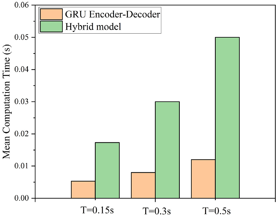
Mean computation times of the GRU-ED, the hybrid model.
Conclusion
There are many difficulties in multi-step prediction for dynamic systems because the unmodeled parts of the system and the noise in the data lead to error accumulation and reduce the prediction accuracy. For vehicle dynamic systems, this problem is particularly important because the vehicle’s driving conditions are affected by many complex phenomena. It is not easy to accurately model these phenomena with physical models. However, data-driven modeling provides more inexplicability because the weight parameters of the network cannot correspond to the parameters of the physical model. In this work, we present a hybrid vehicle model based on the single-track model and GRU neural network to model the lateral vehicle dynamics. In order to capacitate the GRU neural network for accurate long-term predictions with feedback input values, a two-stage learning algorithm is employed, including open-loop and closed-loop training. The prediction accuracy of the hybrid vehicle model is evaluated based on the data collected by the vehicle in the real environment. On all datasets, the hybrid model obtains the best results compared to the single-track model and GRU-ED architecture. The analysis shows that the GRU neural network learns the single-track model’s inaccuracies and provides an error value to compensate for the difference between the measured values. The accurate modeling results can be used as reliable information in automatic driving tests and calibration.
There are various challenges to overcome to reach a robust modeling scheme based on neural networks. While this work provides an accurate modeling technique, future work will improve the results. A grid search or any other advanced method should be used to search the hyperparameters space. Furthermore, improving the quality of training data will potentially increase the overall robustness of the model.
Footnotes
Declaration of conflicting interests
The author(s) declared no potential conflicts of interest with respect to the research, authorship, and/or publication of this article.
Funding
The author(s) disclosed receipt of the following financial support for the research, authorship, and/or publication of this article: This work was supported in part by the National Natural Science Foundation of China (U20A20333, 52072160, 51875255, U1764264), Key Research and Development Program of Jiangsu Province (BE2019010-2, BE2020083-3), Jiangsu Province’s six talent peaks (TD-GDZB-022).