Sage Journals: Discover world-class research

Abstract

A test scenario generation method based on combinatorial testing (CT) and Bayesian Network for autonomous vehicles is proposed in this paper. Firstly, some parameters are selected to describe the test scenarios which are classified according to road types and driving tasks. Then, the constraint sets for the scenarios with forbidden tuples are established to avoid the generated cases do not conform to the reality, in which the construct constraint set (CCS) algorithm is utilized to compute implied constraints. Furthermore, the Bayesian networks is used as the probabilistic models of the scenarios, where the traffic participants are represented as object nodes and the relative relationships between the participants are converted into the network structures. Finally, an improved automatic efficient test case generator (AETG) is developed to generate test cases. By considering both probability and frequency, the select function is designed for determining the values of scenario parameters. And the generation mode can be changed by modifying the weight and target parameters. The effectiveness of the proposed method is evaluated by generating six typical test scenarios. Compared with other algorithms, the numbers of test cases in the sets generated by this method are less and the probability deviations are smaller.

Keywords

Autonomous vehicles automatic testing test scenario generation combinatorial testing Bayesian networks

Introduction

With the rapid development of artificial intelligence technology, more and more vehicles have automated driving functions, which have led to lots of discussions on the safety issues about it.¹ Although automated driving technology can avoid some traffic accidents, it brings new risks to driving behavior.² For this reason, before many autonomous vehicles are put on the market, various tests are required to verify their safety and reliability.

Based on the mortality rate of vehicle accident, at least 240 million kilometers of road test without fault is required to prove an autonomous vehicle is safe and reliable.³ When a fault occurs during the test, the mileage will continue to increase. Therefore, it is difficult to use only road test to verify the safety of autonomous driving. The simulation scenario test method will shorten the test cycle.⁴

There are many types of scenarios, including: driving test scenario,⁵ illegal scenario,⁶ normal scenarios,⁷ and generated scenarios.⁸ The driving test scenarios are derived from the driving test projects.⁹ The scenarios are representative, but there are few types. It is not possible to conduct comprehensive tests on autonomous vehicles.

The illegal scenario^6,10 is a special kind of scenario in which there are traffic participants violating traffic laws. Illegal scenarios can test how autonomous vehicles work when other traffic participants violate traffic laws. However, it is not convenient to use illegal scenarios to build a large-scale scenario library, because the semantic information in the documents is difficult to process in batch.

The normal scenarios are obtained by collecting the traffic environment of the real world. Some normal scenario libraries have been established.^7,11–14 Using normal scenarios to test autonomous vehicles can make the test content closer to the real-world traffic environment. However, the collection of normal scenarios requires numerous drivers to drive vehicles equipped with various instruments on the real road. The cost is high and it takes a long time. Furthermore, there are a large number of repeated scenarios in the collected scenarios, which results in low efficiency.

Most scenarios are collected from real-world, except the generated scenarios which are simulated in the computer. In order to obtain a large number of scenarios quickly and conveniently, several test scenario generation methods have been proposed. A new test case can be obtained by changing the combination of parameter values in the scenarios. Therefore, a type of scenario library could have a large number of test cases, but it is impossible for an autonomous vehicle to perform all case tests. Rocklage et al.¹⁵ used the CT method to generate test cases for scenarios, which can greatly reduce the size of the scenario libraries and improve test efficiency. However, there are some constraints between parameters in complex scenarios, and some combinations of parameter values do not meet the real situations, which need to be avoided during the generation process.

The CT method is widely used in software testing, which generates a set of test cases by choosing a smaller combinations of parameter value. And now there are many CT tools that can be directly used to generate test cases. For example, Xia et al.¹⁶ used the PICT (pairwise independent combinatorial testing tool) to generate test cases. Khastgir et al.¹⁷ used the Vital (constrained randomization engine) to generate test cases. With the help of these tools, test cases can be quickly generated without to write the CT program.

The above studies are all dedicated to generating a smaller test case set to achieve full coverage of parameter combinations, but the results generated are random. Researchers have found that using scenarios with a low probability of occurrence in the real world can perform intensive tests on automated driving to improve test efficiency.¹⁸ However, there is a small proportion of scenarios with small probability in the randomly generated test case set.

In order to solve the above problem, a test scenario generation method combining the CT and the Bayesian network¹⁹ is presented to ensure that the test case set is small in size while the average probability of generating test cases can be adjusted. The motivation of the proposed improved AETG algorithm is that the occurrence probability of the generated test cases can be controlled. Compared with other methods, this method can switch the generation mode by modifying the design parameters. The method can either generate a set of test cases by considering the probability, or only use the CT to generate test cases. The target parameter in the method determines whether the test case with the largest probability or the smallest probability is generated, that is, a probability dependent parameter. It should be pointed out that the scenarios generated by this method do not consider the interaction between objects, because all background objects in the scenarios move according to a predetermined trajectory except for the vehicle under test. The test cases set generated by the improved AETG algorithm can not only include all combinations in the uncovered combination set like the traditional combinatorial test algorithms, but also have more test cases with small occurrence probability when the value of the target parameter is small (i.e. the level of exposure to dangerous events is very high, and the evaluation of the autonomous vehicles is accelerated²⁰). In this study, the algorithm generates a few test scenarios in a short period of time, only a few seconds, which is suitable for repetitive testing of single autonomous driving function, such as automatic parking system test. It is assumed that the motion state of the objects in the test scenarios remains unchanged during testing, and the objects move according to predefined trajectories or remain stationary.

The following sections are organized as follows: Section 2 defines the data structure of the scenario. Section 3 describes how to find the constraints between the parameters of scenario. Section 4 introduces the Bayesian network used to generate the scenario. Section 5 combines the Bayesian network with the AETG to obtain a new test scenario generation method. Section 6 verifies the effectiveness of the proposed method by comparing the test case sets generated by the Combinatorial Testing Based on Complexity (CTBC) algorithm.

Parameters of test scenario

Test scenario can be described by a set of parameters, and different parameters form different scenario test cases. However, not all combinations of the values are reasonable, the unreasonable combinations constitute the constraint set of the test scenario. In order to simplify the model and reduce the calculation workload, some critical parameters are selected to describe the scenarios. The parameters can be divided into three categories: environment, road and object. The framework of the test scenario is shown in the Figure 1 below.

Figure 1.

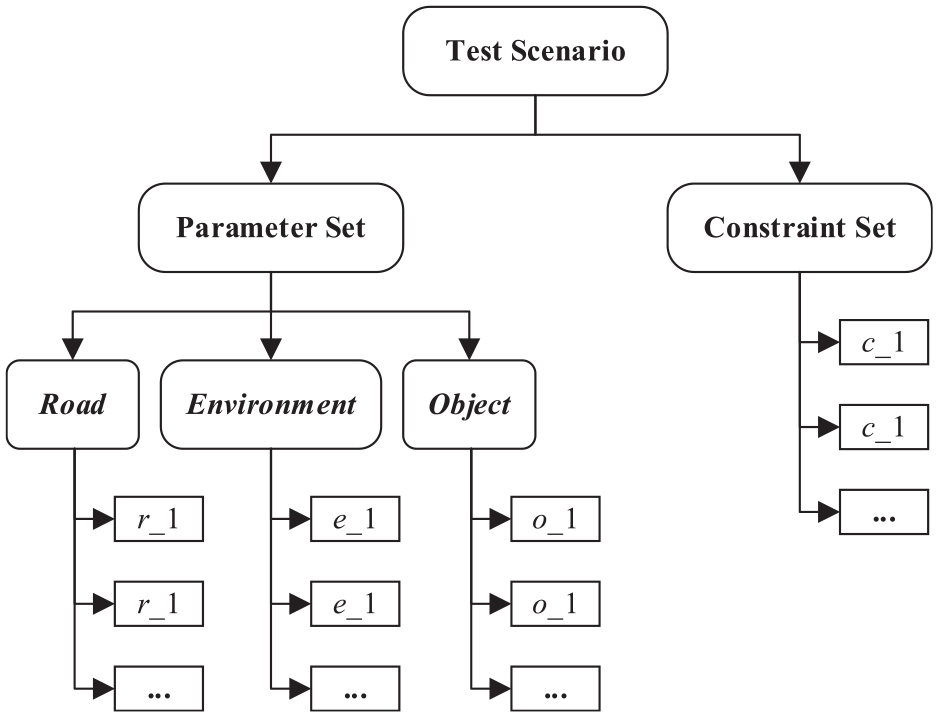
Framework of Test Scenario.

Environment

The environment describes the environmental conditions in the scenario, which include weather, intensity, and light. When using the CT to generate the scenario, the parameters are required to be discrete. Table 1 shows the value ranges of environment. In order to reduce calculation workload during test case generation, only three values for each environment parameter have been determined. The intensity is used to represent the weather intensity in the scenario. For example, when it rains, the greater the intensity, the greater the rainfall. During the simulation test, the environment will affect the sensor model of the tested vehicle. The environment in the scenarios is constant and does not change with time.

Table 1.

Value range of environment.

Weather	Intensity	Light
Cloudy/sunny	Feeble	Daytime
Rain/snow	Medium	Dusk/dawn
Fog	Strong	Night

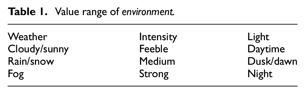
We combine sunny and cloudy into one category of weather parameters, because neither of them has particles in the air to block the detection of the sensor. And we merge rainy and snowy into another category, because the diameters of raindrops and snowflakes are both several millimeters. However, the diameter of the particles for foggy is about less than 100 microns.

Road

The road is used to describe the condition of road segment in the scenarios. A continuous road is divided into several road segments. Taking the Ramp entrance as an example, it can be divided into 4 road segments, as shown in Figure 2.

Figure 2.

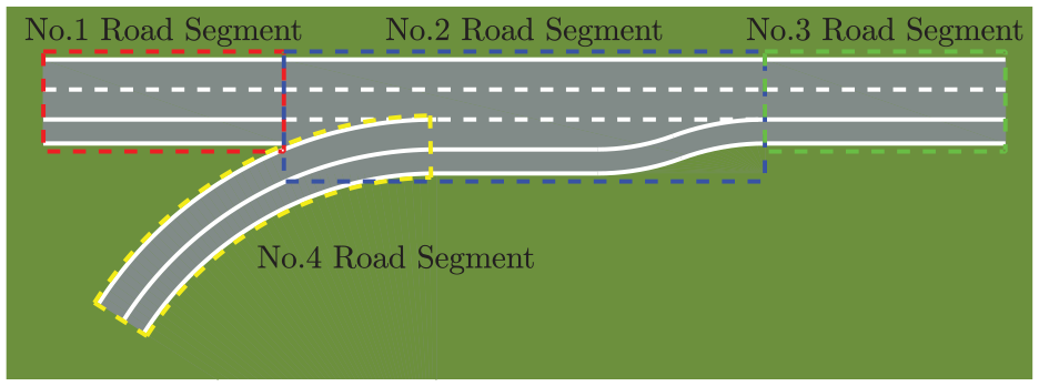
Road segments of ramp entrance.

In order to accurately describe the positions and postures of the road segments in the scenario, a coordinate system on the road segment is established, called the road segment coordinate system (RSCS), as shown in Figure 3. According to the radius, the road segments in the scenario can be divided into two categories: straight road segment and curved road segment. On the straight road segment, a rectangular coordinate system is established, called the straight road segment coordinate system (SRSCS). On the curved road segment, a polar coordinate system is established, called the curved road segment coordinate system (CRSCS). In this paper, the coordinate system of the scenario is called the scenario coordinate system (SCS).

Figure 3.

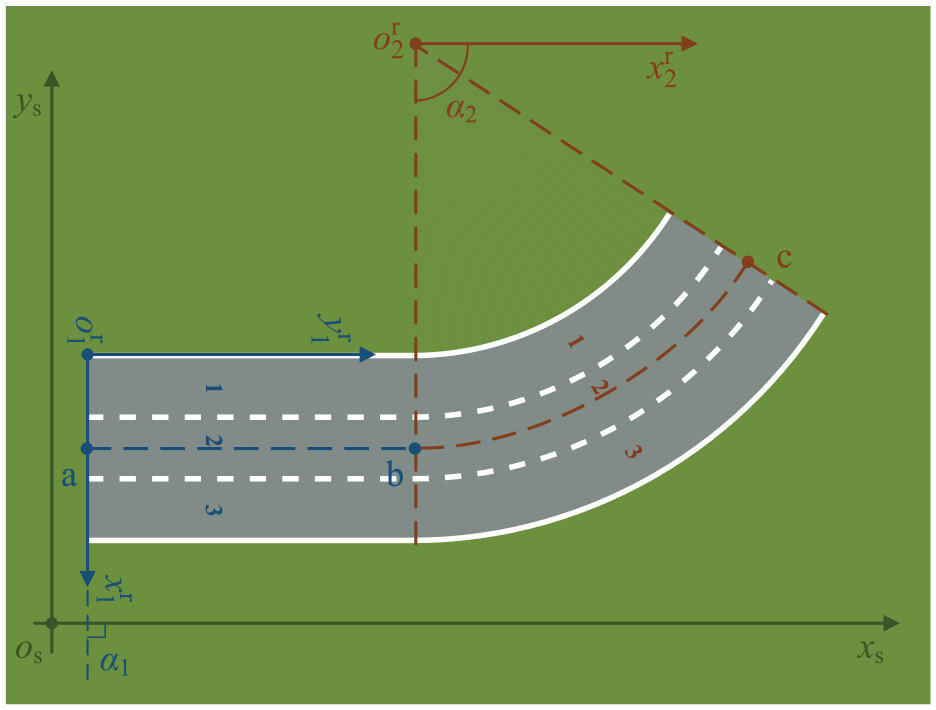
Coordinate system of road segment.

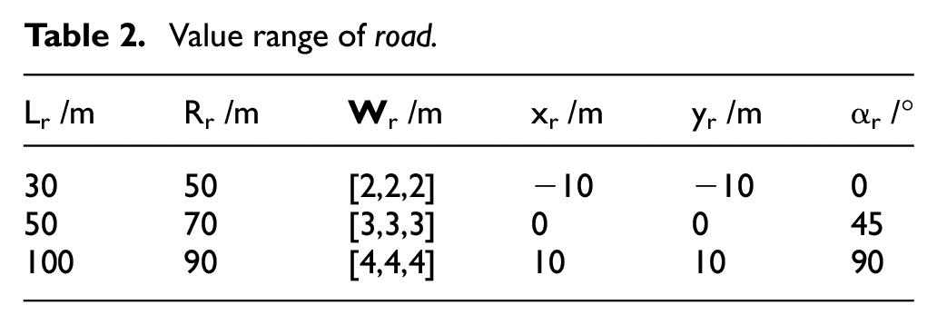
The road includes following parameters: L_r, R_r, W _r, [x_r, y_r], α_r. The L_r is length of the center line on road segment. The R_r is radius of the center line on road segment. The W _r is width of all lanes on road segment. The [x_r, y_r] is coordinate of the origin of RSCS under SCS. The α_r is the angle between SRSCS and SCS or the angle of starting point of the curve road segment in CRSCS. Where, r is the serial number of road segment. Since the condition of road in different scenarios are various, the value ranges of the roads need to be carried out according to the scenario type, and an example is shown in Table 2.

Table 2.

Value range of road.

L_r /m	R_r /m	W _r /m	x_r /m	y_r /m	α_r /°
30	50	[2,2,2]	−10	−10	0
50	70	[3,3,3]	0	0	45
100	90	[4,4,4]	10	10	90

Object

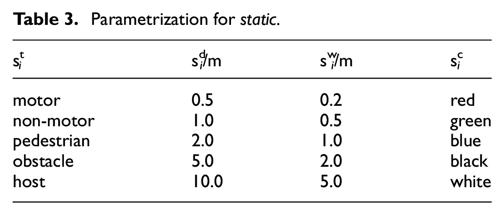
The object records the information of the traffic participant in the scenario, which have two parameters: static and dynamic. The static includes: the type of object $s_{i}^{t}$ , the length of object $s_{i}^{d}$ , the width of object $s_{i}^{w}$ and the color of object $s_{i}^{c}$ , where, i is the serial number of objects. These parameters will not change with time, some discrete points that static can take are shown in Table 3. The traffic participants can be roughly divided into motor vehicle, non-motor vehicle, pedestrian, obstacle, and host vehicle. In this paper, the host vehicle refers to vehicle under test.

Table 3.

Parametrization for static.

s^t_i	s^d_i/m	s^w_i/m	s^c_i
motor	0.5	0.2	red
non-motor	1.0	0.5	green
pedestrian	2.0	1.0	blue
obstacle	5.0	2.0	black
host	10.0	5.0	white

Similar to the RSCS, every object in the scenario also has a coordinate system, called the object coordinate system (OCS), as shown in Figure 4.

Figure 4.

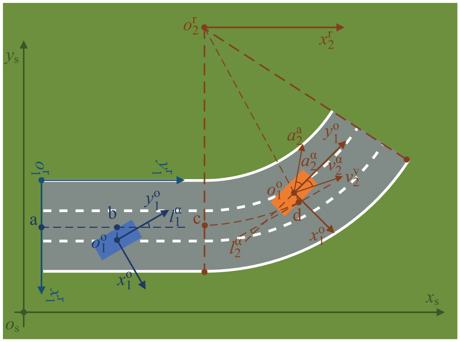
Coordinate system of object.

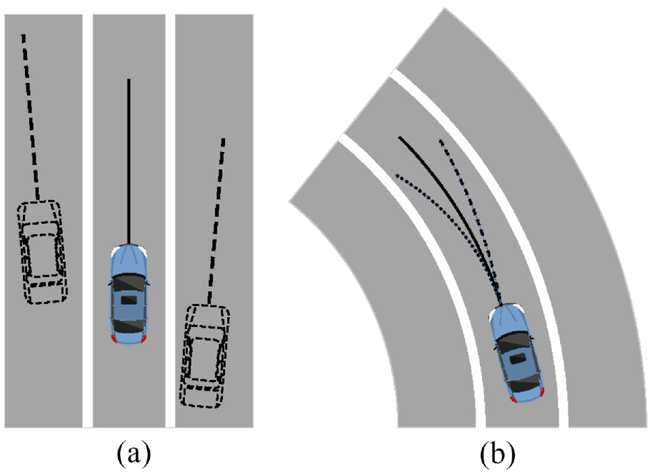
The dynamic describes the movement state of object at the beginning of scenario, which includes: $L_{i}$ = [ $l_{i}^{r}$ , $l_{i}^{e}$ , $l_{i}^{x}$ , $l_{i}^{y}$ , $l_{i}^{α}$ ], $V_{i}$ = [ $v_{i}^{v}$ , $v_{i}^{α}$ ], $A_{i}$ = [ $a_{i}^{a}$ , $a_{i}^{α}$ ]. After the scenarios starting, the host vehicle is controlled by itself, and other objects move according to predetermined trajectories which are defined in the object coordinate system. With the changing of the start position and postural of objects, their trajectories will also translate and rotate, as shown in (a) of Figure 5. Besides, some parameters in the trajectory can also be added to the object parameters, and the trajectory will change in different test cases. For example, the radius in the curve trajectory can be added to the scenario parameters, as shown in (b) of Figure 5.

Figure 5.

Predetermined trajectory of objects: (a) starting position and postural change and (b) radius change.

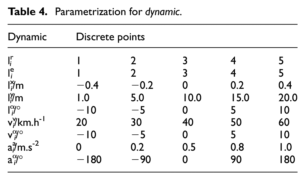
Some discrete points that the dynamic can take are shown in Table 4.

Table 4.

Parametrization for dynamic.

Dynamic	Discrete points
l^r_i	1	2	3	4	5
l^e_i	1	2	3	4	5
l^x_i/m	−0.4	−0.2	0	0.2	0.4
l^y_i/m	1.0	5.0	10.0	15.0	20.0
l^α_i/°	−10	−5	0	5	10
v^v_i/km.h^-1	20	30	40	50	60
v^α_i/°	−10	−5	0	5	10
a^a_i/m.s^-2	0	0.2	0.5	0.8	1.0
a^α_i/°	−180	−90	0	90	180

The $l_{i}^{r}$ is serial number of the road segment where the object is located. The $l_{i}^{e}$ is serial number of the lane where the object is located. The $l_{i}^{x}$ is distance that objects deviate from the centerline of the lane. The $l_{i}^{y}$ is the distance that objects travel along the lane, and it is positive when the objects travel counter clockwise on the curve road segment. The $l_{i}^{α}$ is angle between the y-axis of OCS and the tangent of center line of the lane where the object is located. The $v_{i}^{v}$ is the value of velocity. The $v_{i}^{α}$ is the angle between the direction of velocity and the y-axis of OCS. The definition of $A_{i}$ is similar to $V_{i}$ .

Type of scenario

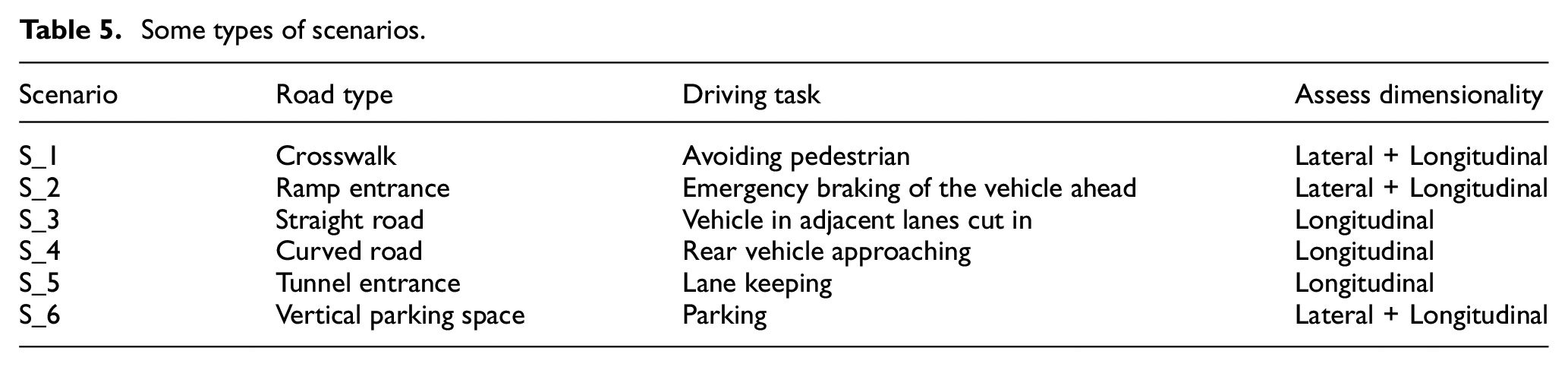
There are many types of scenarios, it is difficult to use a unified framework to generate all types. Therefore, we classify test scenarios based on road type and driving task, and some types of scenarios are shown in Table 5.

Table 5.

Some types of scenarios.

Scenario	Road type	Driving task	Assess dimensionality
S_1	Crosswalk	Avoiding pedestrian	Lateral + Longitudinal
S_2	Ramp entrance	Emergency braking of the vehicle ahead	Lateral + Longitudinal
S_3	Straight road	Vehicle in adjacent lanes cut in	Longitudinal
S_4	Curved road	Rear vehicle approaching	Longitudinal
S_5	Tunnel entrance	Lane keeping	Longitudinal
S_6	Vertical parking space	Parking	Lateral + Longitudinal

In the scenarios, the host vehicle needs to complete some driving tasks. Take the Scenario 1 in Table 5 as an example, the scenario occurs at an ETC. The host vehicle needs to follow the front vehicle through ETC, which mainly to evaluate the longitudinal control capability of the host vehicle. In this paper, we set the roads of each type of the scenarios to constant values, and only use the CT on object and environment to generate the test cases.

In order to display the generated scenarios more intuitively, schematic diagrams of the scenarios are drawn, as shown in Figure 6. Various colored squares are used to represent objects in the scenarios. The white square in the figures represents the vehicle under test, and other vehicles and pedestrians in the scenarios are represented by squares of different colors and sizes.

Figure 6.

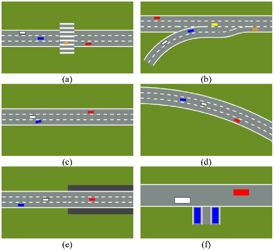
Schematic diagrams of the scenarios: (a) Scenario S_1 (b) Scenario S_2 (c) Scenario S_3 (d) Scenario S_4 (e) Scenario S_5 (f) Scenario S_6.

Constraints in test scenario

There are constraints between various parameters, and the combination of some parameters may not conform to the actual situation (i.e. do not meet the constraints), such as the interference of object position at the beginning of the scenario. To avoid generating such test cases, all constraints need to be listed. Because different types of scenarios are quite different, we establish constraint sets for each scenario one by one.

Initial constraint set

In this paper, the roads in each type of scenario are constant value, and the environment is too simple to ignore the constraints, so we only consider the constraints of objects. The sources of constraints are as follows: no object interference, obstacles keeping stationary, objects do not appear, driving task. All the constraints are represented by forbidden tuples,²¹ which is a method widely used in the CT. For example, in Figure 4, the value range of $l_{1}^{e}$ and $l_{2}^{e}$ is {1,2,3}. If we want these two objects to be located in adjacent lanes, we can get the following forbidden tuple: ∼{ $l_{1}^{e}$ , $l_{2}^{e}$ |1,3}, ∼{ $l_{1}^{e}$ , $l^{e}$ 2|3,1}. The value combinations in the forbidden tuples are forbidden to appear in the test cases.

Some constraints may be difficult to convert directly into forbidden tuples. In this case, they need to be converted into other types of tuples firstly, such as must tuples,²² and then converted into forbidden tuples. For example, in Figure 4, if the No. 1 object is an obstacle, it needs to keep stationary, and the speed and acceleration are both 0. The must tuple is as follows:

{s_{1}^{t} | obstacle} \to {v_{1}^{v}, v_{1}^{α}, a_{1}^{a}, a_{1}^{α} | 0, 0, 0, 0}

(1)

Exclude the value combinations in must tuples from all the value combinations of the $v_{1}^{v}$ , $v_{1}^{α}$ , $a_{1}^{a}$ , and $a_{1}^{α}$ to get the forbidden tuples. Assuming that the value ranges of $v_{1}^{v}$ , $v_{1}^{α}$ , $a_{1}^{a}$ , and $a_{1}^{α}$ is {0,10},{0},{0,1} and {0}, the forbidden tuples converted from (1) is:

\begin{matrix} ~ {s_{1}^{t}, v_{1}^{v}, v_{1}^{α}, a_{1}^{a}, a_{1}^{α} | obstacle, 0, 0, 1, 0} \\ ~ {s_{1}^{t}, v_{1}^{v}, v_{1}^{α}, a_{1}^{a}, a_{1}^{α} | obstacle, 10, 0, 0, 0} \\ ~ {s_{1}^{t}, v_{1}^{v}, v_{1}^{α}, a_{1}^{a}, a_{1}^{α} | obstacle, 10, 0, 1, 0} \end{matrix}

(2)

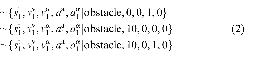
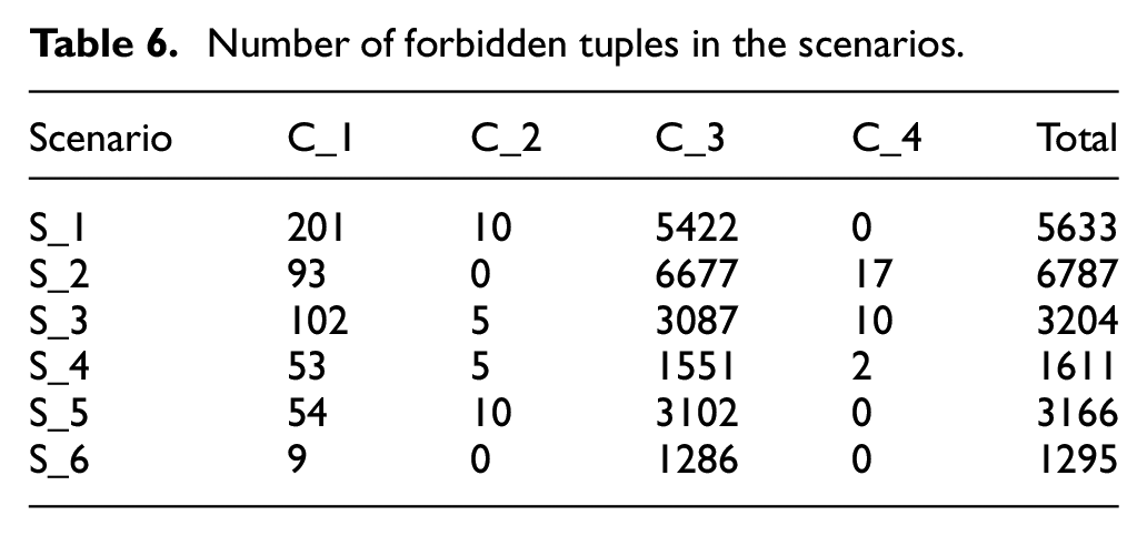
Table 6 shows the number of forbidden tuples in the scenarios of Table 5. Each column represents the number of forbidden tuples converted from a constraint. The C_1 is the constraint that no object interference, the C_2 is the constraint that obstacles keeping stationary, the C_3 is the constraint that objects do not appear, the C_4 is the constraint that driving task. The last column is the total numbers of forbidden tuples.

Table 6.

Number of forbidden tuples in the scenarios.

Scenario	C_1	C_2	C_3	C_4	Total
S_1	201	10	5422	0	5633
S_2	93	0	6677	17	6787
S_3	102	5	3087	10	3204
S_4	53	5	1551	2	1611
S_5	54	10	3102	0	3166
S_6	9	0	1286	0	1295

The initial constraint set is generated by converting various constraints into forbidden tuples. The road type and driving task may be different from each scenario, so the initial constraint set is not universal. In order to control the size of the initial constraint set, the number of objects in the scenario was reduced as much as possible. If the range of the parameters are expanded or the number of objects increases, the size of the initial constraint set will increase rapidly, which will lead to a long time for the generation of test cases.

Implied forbidden tuple

If a forbidden tuple c is induced by other forbidden tuples, then c is an implied forbidden tuple. Suppose there are parameters {a, b, c}; a, b, c∈{1, 2}; forbidden tuples set {∼{a,c|(2,−,2)}, ∼{b,c|(-,2,1)}}. When parameters a = 2, b = 2, it can be inferred that the value range of parameter c is empty. Therefore, the implied forbidden tuple ∼{a,b|(2,2,-)} must be added to the forbidden tuples set.

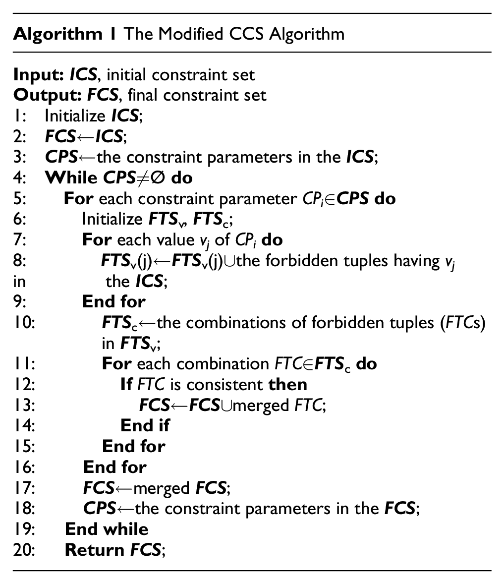
Ignoring implied forbidden tuples may lead to some invalid test cases, which further leads to inaccurate test planning and wasted effort. There are usually implied forbidden tuples in the initial constraint set, and an algorithm is needed to find them. In this paper, we use the modified construct constraint set (CCS) algorithm²³ to search for the implied forbidden tuples. The algorithm looks for the constraint parameters after each implied constraint search to avoid the implied constraints from generating new constraint parameters, not just at the beginning. The search for implied constraints will not end until there are no new constraint parameters.

Now, the modified CCS algorithm is introduced in detail as shown below. Only the constraint set that does not contain implied constraints can be used for the test case generation, otherwise it may cause the parameter range empty when the test case is generated.

Algorithm 1 The Modified CCS Algorithm
Input: ICS, initial constraint set
Output: FCS, final constraint set
1: Initialize ICS ; 2: FCS ← ICS ; 3: CPS ←the constraint parameters in the ICS ; 4: While CPS≠Ødo 5: For each constraint parameter CP_i∈CPS do 6: Initialize FTS _v, FTS _c; 7: For each value v_j of CP_i do 8: FTS _v(j)← FTS _v(j)∪the forbidden tuples having v_j in the ICS ; 9: End for 10: FTS _c←the combinations of forbidden tuples (FTCs) in FTS _v; 11: For each combination FTC∈ FTS _cdo 12: IfFTC is consistent then 13: FCS ← FCS ∪merged FTC; 14: End if 15: End for 16: End for 17: FCS ←merged FCS ; 18: CPS ←the constraint parameters in the FCS ; 19: End while 20: Return FCS;

Construction of Bayesian network

In this paper, the Bayesian network is used to calculate the probability of parameter values under different conditions. For different scenarios, the parameters and constraints are different, so the Bayesian network is also different. Because the road and environment are relatively simple, we assume that their parameters obey an independent and uniform distribution, and the Bayesian network is mainly used to calculate the probability of the objects.

Structure of Bayesian network

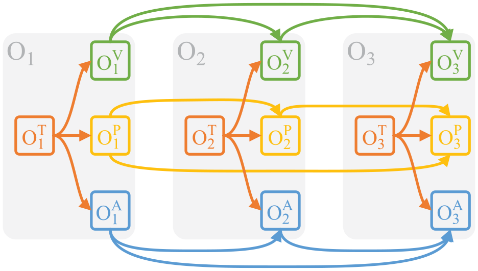
In the Bayesian network, object node represents the object in the scenario, which contains parameter nodes: type node, position node, velocity node and acceleration node. Figure 7 shows the Bayesian network of S_3, where $O_{i}$ is the object node, $O_{i}^{T}$ is the type node, $O_{i}^{P}$ is the position node, $O_{i}^{V}$ is the velocity node, $O_{i}^{A}$ is the acceleration node, i∈(1,2,3).

Figure 7.

Bayesian network of S_3.

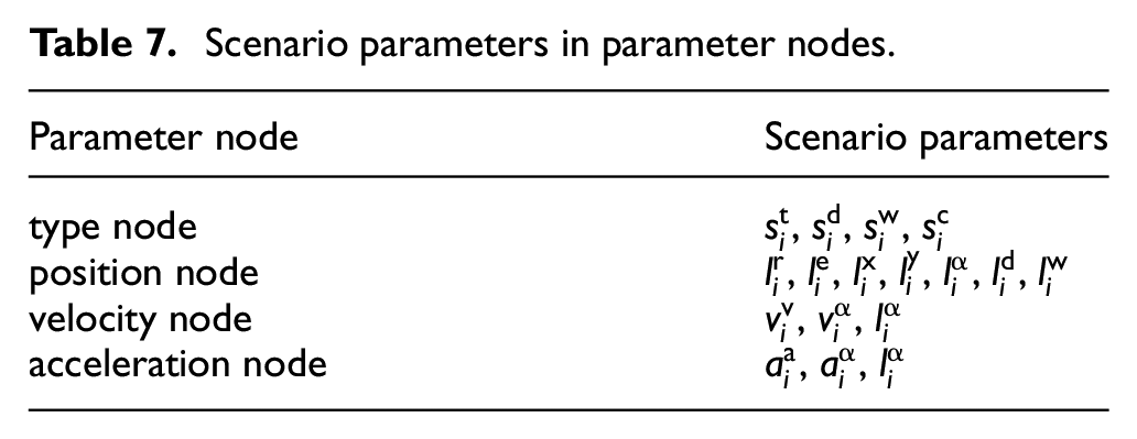
The parameter nodes contain several scenario parameters as shown in Table 7, and the value of the nodes are combinations of the parameter values.

Table 7.

Scenario parameters in parameter nodes.

Parameter node	Scenario parameters
type node	$s_{i}^{t}$ , $s_{i}^{d}$ , $s_{i}^{w}$ , $s_{i}^{c}$
position node	$l_{i}^{r}$ , $l_{i}^{e}$ , $l_{i}^{x}$ , $l_{i}^{y}$ , $l_{i}^{α}$ , $l_{i}^{d}$ , $l_{i}^{w}$
velocity node	$v_{i}^{v}$ , $v_{i}^{α}$ , $l_{i}^{α}$
acceleration node	$a_{i}^{a}$ , $a_{i}^{α}$ , $l_{i}^{α}$

In object nodes, due to the lack of real data of various scenarios, the probability distribution of type nodes is simplified to independent and uniform distribution, which contains object parameters: type, color, length and width, and is the parent node of other parameter nodes. We use distance interaction, velocity interaction, and acceleration interaction to represent the interaction between object nodes, and the Bayesian network shown in Figure 7 is used to represent these interactions. In order to quantify the interaction, a series of relative parameters are defined. The relative distance is the minimum distance between the bounding boxes of two objects, and the relative velocity (acceleration) is the vector sum of the velocities (acceleration) of two objects.

Conditional probability

The conditional probability of Bayesian network usually needs to be trained based on a large amount of statistical data. However, due to the lack of data, we used the method of mapping relative parameters to probability, as shown below.

There are some models that use relative distance, relative speed and relative acceleration to quantify the risk of driving environment, such as Driving Risk Field (DRF)^24,25 and Enhanced Time to Collision (ETTC).^26,27 Since the probability of dangerous scenarios in real driving environment is usually low, we assume that there is a correlation between the probability and the driving environmental risk, and the relative parameters can be used to map the conditional probability.

Initialize the range of unvalued parameter node node as v ={v₁, v₂, …, v_n};

Find the valued parameter nodes of the same type as node, get Node ={node₁, node₂, …, node_i}, and the process of node value selecting are shown in Algorithm 3;

Calculate relative parameter (relative distance, relative velocity and relative acceleration) between node and Node , and get the relative parameter matrix RPM ={rp₁, rp₂,…, rp _i};

Calculate the mean and standard deviation of each row in the RPM as r _m, r _d;

Map r _m, r _d to probability, as shown in (3), get pro _m, pro _d;

Calculate the average of pro _m, pro _d to get the conditional probability of node as Pro , as shown in (4).

It is very difficult to obtain the marginal probability distribution and conditional probability distribution in the real world, because there are so many scenario parameters and most of them are difficult to collect.

Due to the lack of real data, we simplified the probability distribution function. And in this paper, we focus on the construction of test cases generation algorithm rather than the acquisition of probability distribution. When mapping r _m, r _d to probabilities, the probability distribution chosen in this paper is triangular distribution,²⁸ and its probability density function is shown in (3). When mapping the r _m to the pro _m, set c = (a+b)/2. When mapping the r _d to the pro _d, set c = a.

f (x, a, b, c) = {\begin{matrix} \frac{2 (x - a)}{(b - a) (c - a)} & a \leq x \leq c \\ \frac{2 (b - x)}{(b - a) (b - c)} & c \leq x \leq b \end{matrix}

(3)

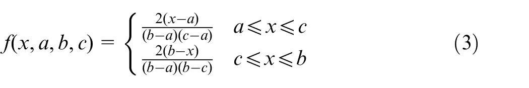
Where, a is the minimum value of x, b is the maximum value of x, and c is the value of x corresponding to the triangle vertex.

The r _m, r _d are respectively substituted into their probability density functions to obtain column vectors y _m, y _d. Finally, the y _m, y _d are used to calculate Pro , as shown in (4).

Pro = \frac{pr o_{m} + pr o_{d}}{2} = \frac{y_{m} / \sum_{i = 1}^{n} y_{m} (i) + y_{d} / \sum_{i = 1}^{n} y_{d} (i)}{2}

(4)

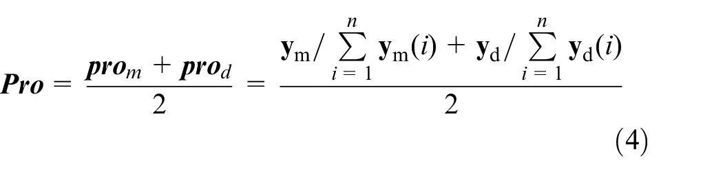
Where, n is the length of vector y _m, y _d.

Scenario generation algorithm

If all the combinations of parameters are put into a test case set, a very large test case set will be obtained because the number of parameters in the scenario is huge, it is difficult to traverse this test case set. In this paper, we use the CT to reduce the size of test case set. The CT is widely used in the software testing, aiming to select a small number of test cases from the huge combination space to improve the test efficiency. The current common test case generation algorithms include: the automatic efficient test case generator (AETG),²⁹ the test case generator (TCG),³⁰ and the in-parameter order, (IPO)³¹ etc.

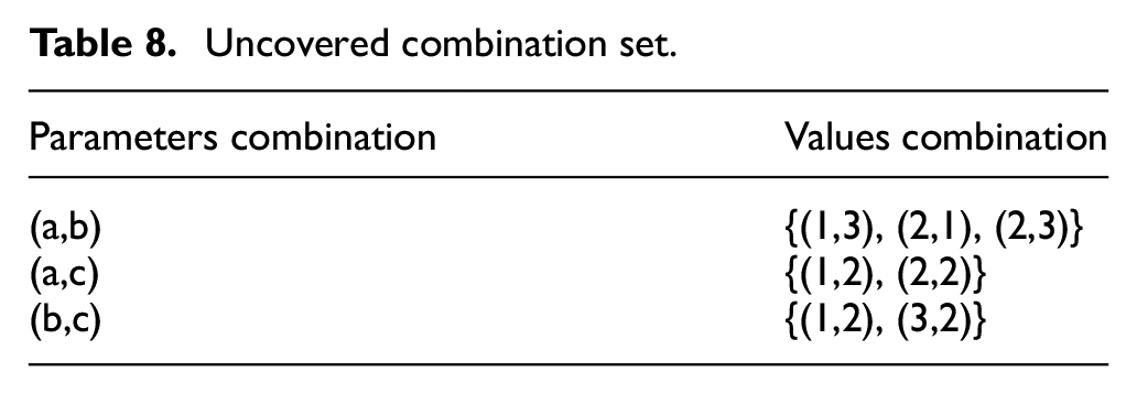
Uncovered combination set

Before using the test case generation algorithms to generate test cases, it is necessary to generate an uncovered combination set, and the generated test case set should include all combinations in the uncovered combination set. The uncovered combination set is any values combination of any n_U parameters that satisfy the constraints, where n_U is the wise of uncovered combination set. For example, suppose there are parameters a,b,c, the value range is {(a|1,2), (b|1,3), (c|2,3)}, and the constraint is ∼{a,b|1,1}, ∼{c|3}, ∼{a,b,c|2,3,2}. When n_U = 2, the uncovered combination set is shown in Table 8.

Table 8.

Uncovered combination set.

Parameters combination	Values combination
(a,b)	{(1,3), (2,1), (2,3)}
(a,c)	{(1,2), (2,2)}
(b,c)	{(1,2), (3,2)}

Algorithm 2 Frequency calculation algorithm
Input: case, test case being generated; par _c=[ ${par}_{1}^{c}, {par}_{2}^{c} . . ., {par}_{i - 1}^{c}$ ], valued parameters in case ; v _c=[ $v_{1}^{c}, v_{2}^{c} . . ., v_{i - 1}^{c}$ ], values of par _c; par _n=[ ${par}_{1}^{n}, {par}_{2}^{n} . . ., {par}_{i - 1}^{n}$ ], parameters in unvalued parameter node; V _n=[ $v_{1}^{n}, v_{2}^{n} . . ., v_{m}^{n}$ ], value range of par _n; U , uncovered pair-wise combination set; n_U, the wise of U
Output: f _n, value frequency of par _n
1: Initalize f _n; 2: For each value $v_{j}^{n}$ ∈ V _ndo 3: For each parameter ${par}_{l}^{n}$ ∈ par _ndo 4: Ifl>1 then 5: par _c= par _c∪ ${par}_{l}^{n}$ ; 6: v _c = v _c∪ $v_{l}^{n}$ (l-1); 7: End if 8: Select n_U-1 parameters from par _c, and put all the parameter selection combinations into Com _p; 9: According to Com _p and v _c, get Com _v (the combination of values); 10: For each combination Com _p(q)∈ Com _pdo 11: If find combination ( Com _p(q), ${par}_{l}^{n}$ Com _v(q), $v_{l}^{n}$ (l)) in U then 12: f _n(j)= f _n(j)+1; 13: End if 14: End for 15: End for 16: End for 17: f _n= f_n/∑f_n;

Algorithm 3 The improved AETG algorithm
Input: par _s=( ${par}_{1}^{s}, {par}_{2}^{s} . . ., {par}_{n}^{s}$ ), the parameters in the scenario; $V_{s} = (v_{1}^{s}, v_{2}^{s}, . . ., v_{n}^{s})$ , the value range of par _s; U , the uncovered pair-wise combination set; Par _n=( ${par}_{1}^{n}, {par}_{2}^{n} . . ., {par}_{m}^{n}$ ), the parameter nodes in the scenario; FCS , the final constraint set; n_c, number of the candidate test cases; α, the weight; p_e, the target parameter
Output: Case, test case set
1: While U≠Ødo 2: Initalize the candidate test case set, get Case_c; 3: Initalize α; 4: For each candidate test case ${case}_{i}^{c}$ in Case _cdo 5: For each parameter node ${par}_{j}^{n}$ in Par_ndo 6: Find the value range of par _n according to V _s, ${case}_{i}^{c}$ and FCS , get V _n; 7: Calculate the value frequency of ${par}_{j}^{n}$ according to U, V_n and ${case}_{i}^{c}$ , get f _n; 8: Calculate the value probability of ${par}_{j}^{n}$ according to V _n and ${case}_{i}^{c}$ , get p _n; 9: Calculate the selection function of ${par}_{j}^{n}$ according to α, p_e, f_n and p_n, get s_n; 10: Find the minimum value in s _n, get s _n(l); 11: Use V _n(l,:) as the value of ${par}_{l}^{n}$ ; 12: End for 13: End for 14: Find the candidate test case that cover U the most, get case _c; 15: U = U - U ∩ case _c; 16: If the size of U has not decreased then 17: Increase α, and skip to step 4; 18: End if 19: Case = Case ∪ case _c; 19: End while

As the n_U increase, the number of uncovered combinations will increase rapidly, which will lead to a longer time to complete the test case generation, as shown in Figure 8. Kuhn and Reilly.³² found that software errors are mostly caused by the interaction of several parameters, and more than 70% of errors are triggered by the interaction of two parameters. So, we decide to make n_U = 2, and use uncovered pair-wise combination set to generate test cases.

Figure 8.

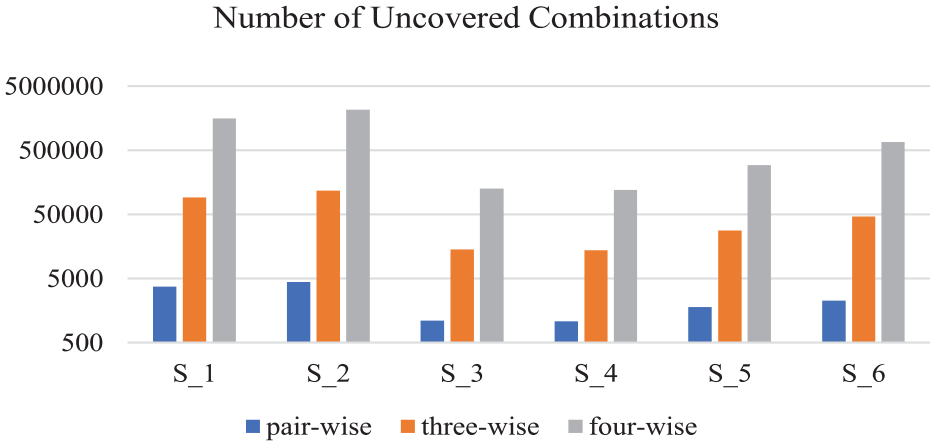
Number of uncovered combinations.

Selection function

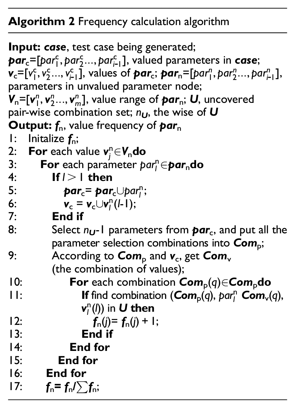
In AETG, which value of the scenario parameter is selected to form the test case depends on the number of times that the value appears in the uncovered pair-wise combination set,³³ and the value with the highest frequency will be preferred. The frequency calculation algorithm used in this paper is as follows.

In order to make the test case generation process affected by the probability, the selection function is used as an indicator to determine the values of the scenario parameters, as shown in (5).

s_{node} = α N (1 - f_{node}) + (1 - α) N (| N (p_{node}) - p_{e} |)

(5)

N (x) = {\begin{matrix} \frac{x - x_{min}}{x_{max} - x_{min}} & x_{max} \neq x_{min} \\ \frac{x}{\sum_{i = 1}^{n_{x}} x (i)} & x_{max} = x_{min} \end{matrix}

(6)

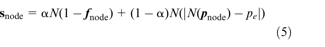
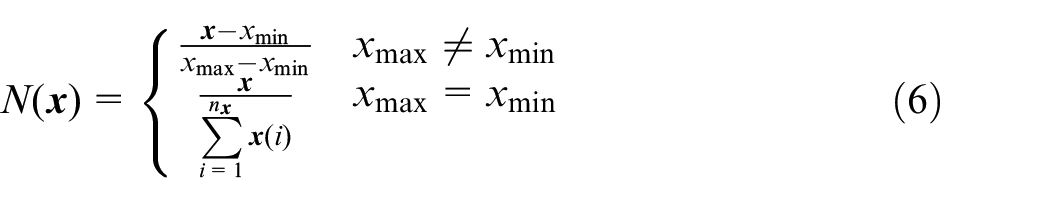
Where, the α is the weight, 0 ≤ α ≤ 1, as α increases, the test case generation process is more affected by the frequency and less affected by the probability. The p_e is target parameter, 0 ≤ p_e≤ 1, it is a probability dependent parameter which represents the ratio of the expected test case probability to all test case probabilities and. N( x ) is the normalization function, x_min is the minimum value in the vector x , x_max is the maximum value in the vector x , and n_x is the length of the vector x .

Test case generation

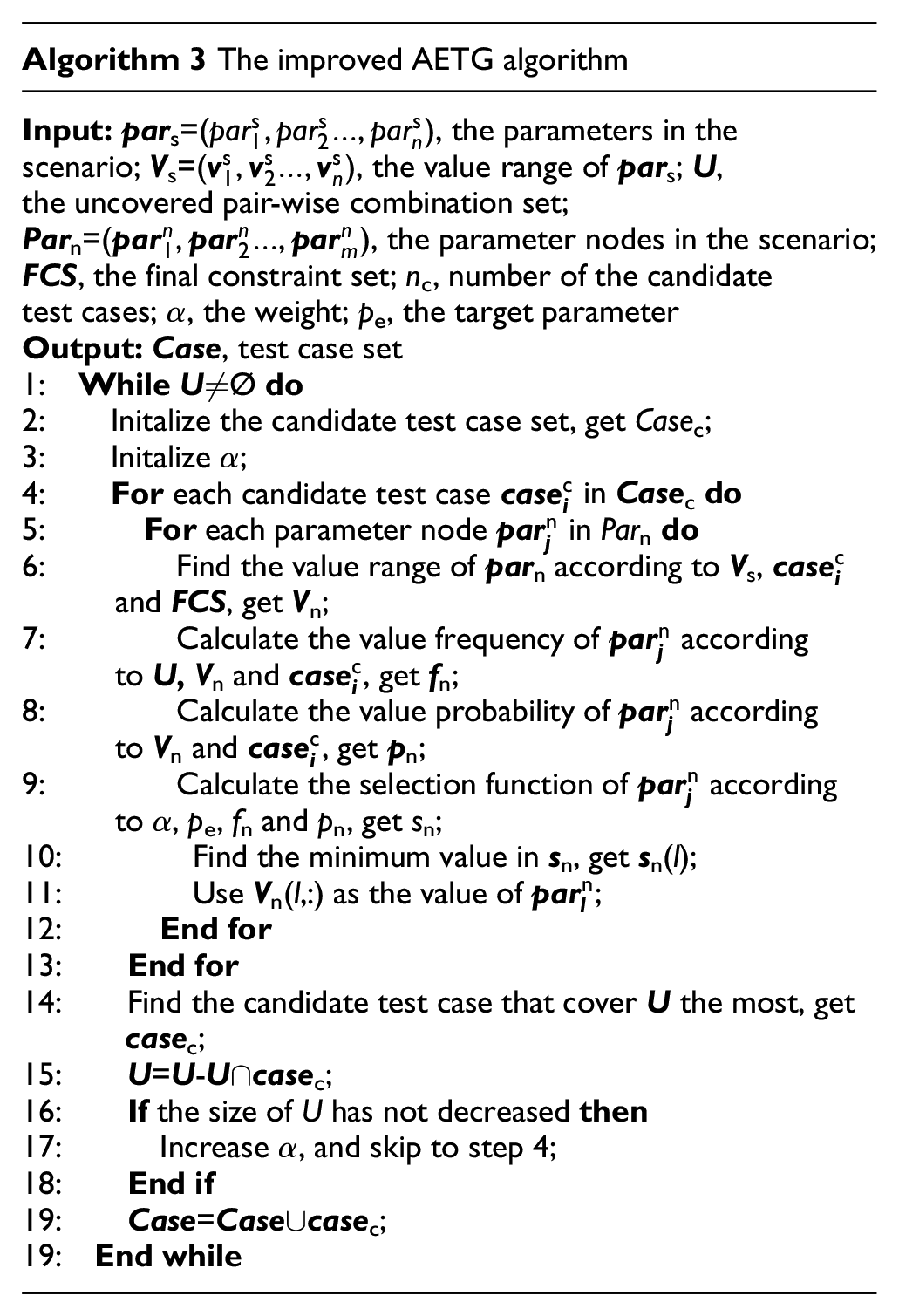
The AETG algorithm is one of the most common test case generation algorithms. When the AETG algorithm works, test cases containing uncovered combinations will be generated one by one, and the parameters in the test cases will be valued one by one. We replace the selection indicator of scenario parameters in the algorithm with selection function, and the improved AETG algorithm is shown in Algorithm 3.

In the process of generating test cases, for the node par ⁿ_j that has no value, firstly, it is necessary to determine its value range V _n, then calculate the selection indicator s _n, and finally, take the value corresponding to the minimum in s _n as the value of the node par ⁿ_j. With the generation of test case, the number of the valued parameter nodes is increasing.

When Algorithm 3 runs to the later stage of test case generation, if the value of α is too small, it is possible to always generate case _c without covering U . If the value of α remains unchanged at this time, the generation process will fall into an infinite loop. So, after completing the generation of Case _c, Algorithm 3 will determine whether the size of U is reduced. If the size of U does not change, Algorithm 3 will adaptively increase the value of α, and then repeat the generation of Case _c.

Result of scenario generation

In order to analyze the impact of weight α and target parameter p_e on the generated results, the improved AETG algorithm is used to generate test cases using different α and p_e. In addition, we compared the generated results with the CTBC algorithm.³⁴

Probability deviation

In order to verify the improved AETG algorithm can generate test cases close to the expected probability, we designed a test scenario with a smaller parameter space based on the S_6 scenario. All test cases in the parameter space are found, and then the Bayesian network is used to calculate their respective probabilities. The expected probability is the probability that target parameter p_e corresponds to the probabilities of all test cases, as shown in (7).

p_{e}^{g} = p_{min}^{g} + (p_{max}^{g} - p_{min}^{g}) p_{e}

(7)

Where, the $p_{e}^{g}$ is expected probability. The $p_{\min}^{g}$ is the minimum of all test case probabilities. The $p_{\min}^{g}$ is the maximum of all test case probabilities.

The probability deviation is used to measure the degree of deviation of test case probability from the expected probability, as shown in (8).

p_{d}^{g} = N (| p^{g} - p_{e}^{g} |)

(8)

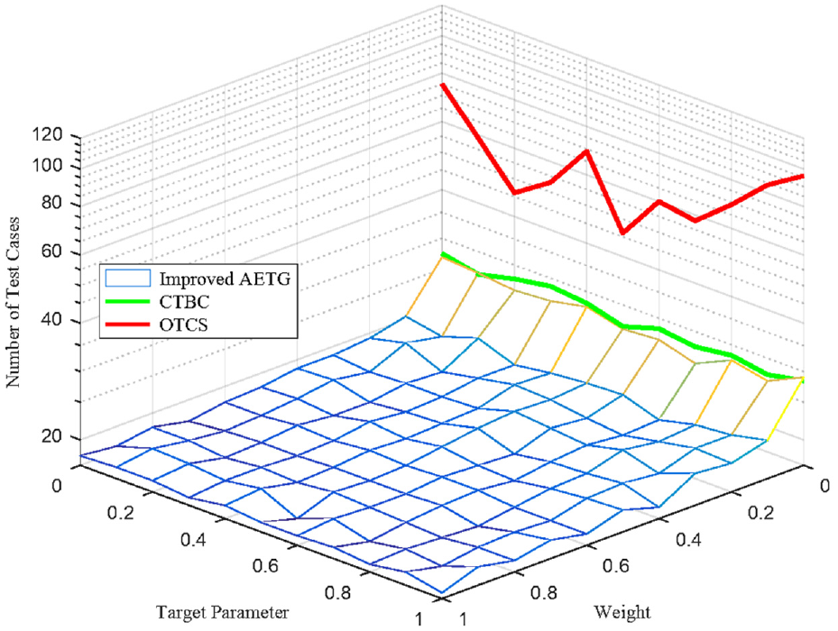
Where, the $p_{c}^{g}$ is probability deviations of all test cases, and the p ^g is all test case probability.

Now, an optimal test case set (OTCS) that can cover all uncovered combinations with the smallest probability deviation can be found. The probability deviations of the test case sets generated by the improved AETG algorithm and the CTBC algorithm when the target parameter p_e and the weight α both change from 0 to 1 are compared with the probability deviations of OTCS, as shown in Figure 9.

Figure 9.

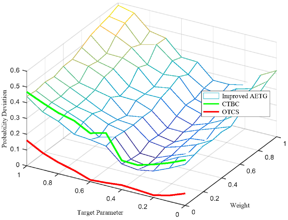
Probability deviations of the test case sets in the test scenario with a smaller parameter space.

In Figure 9, the probability deviations belonging to CTBC and OTCS are represented as curves because they are not affected by weights. It can be seen from Figure 9 that the probability deviations of OTCS are the smallest among the three algorithms, and it is always less than 0.2. However, OTCS can only be applied to the test scenario with a small parameter space, and the computation will increase sharply as the parameter space increases.

If only the influence of the target parameters is considered, it can be found that when p_e is between 0.3 and 0.4, the probability deviation of the test case set generated by the three algorithms is very small. As the target parameters increase or decrease, the probability deviations will increase. The main reason for this phenomenon is the probability deviation distribution of the test cases in the parameter space. Figure 10 shows the number of test cases with different probability deviations in the parameter space when the target parameter changes from 0 to 1. In the defined small parameter space, the probability of most test cases is close to the expected probability when the target parameter is 0.3 or 0.4.

Figure 10.

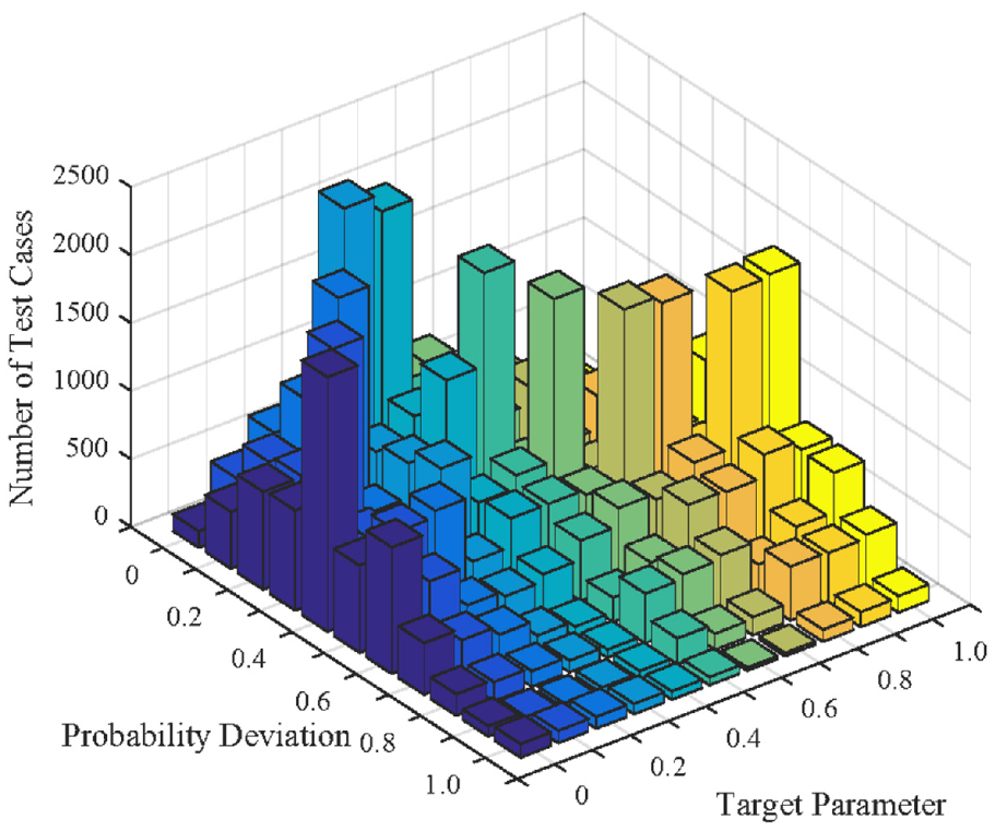
Probability deviation distribution of the test cases in the parameter space.

For the improved AETG algorithm, the probability deviations of the generated test case sets will gradually increase with the increase of weight. The weight determines the influence of probability and frequency on the test case generation, as shown in (5). If the weight is 1, the frequency has the greatest impact on the algorithm, resulting in a large probability deviation of the generated test case set.

When the target parameter p_e = 0.3 and the weight α changes from 0 to 1, the probability deviations of the test case sets generated by the improved AETG algorithm and the CTBC algorithm are shown in Figure 11. In the figure, the probability deviation of the optimal test case set is about 0.02. The CTBC algorithm is not affected by the weight, and the probability deviation is always about 0.18. With the increase of the weight, the probability deviation of the test case sets generated by the improved AETG algorithm becomes larger. Compared with the CTBC algorithm, the probability deviations of test case sets generated by improved AETG algorithm is slightly smaller when the weight is less than 0.5.

Figure 11.

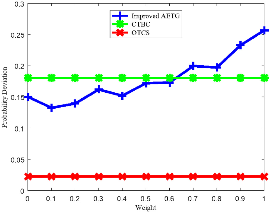
Influence of weight on probability deviation (α = 0–1, p_e = 0.3).

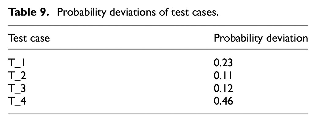
In order to verify the accuracy of the probability deviation calculation, some test cases are selected to judge the probability subjectively based on the schematic diagrams, and the judgment results were compared with the calculated values. Four test cases are randomly selected from the test case sets where the weight α = 0.2 and the target parameter p_e = 0.3, the probability deviations are shown in Table 9.

Table 9.

Probability deviations of test cases.

Test case	Probability deviation
T_1	0.23
T_2	0.11
T_3	0.12
T_4	0.46

The schematic diagrams of the test cases are shown in Figure 12. In the scenario, all objects remain static at the beginning, so the probabilities of the test cases are only related to relative distances between the objects. The relative distances in Bayesian network includes: the relative distance between the vehicle under test and the object in left parking space, the relative distance between the vehicle under test and the obstacle on the road, the relative distance between the objects in the left and right parking spaces, the relative distance between the objects in the left/right parking spaces and the obstacle on the road.

Figure 12.

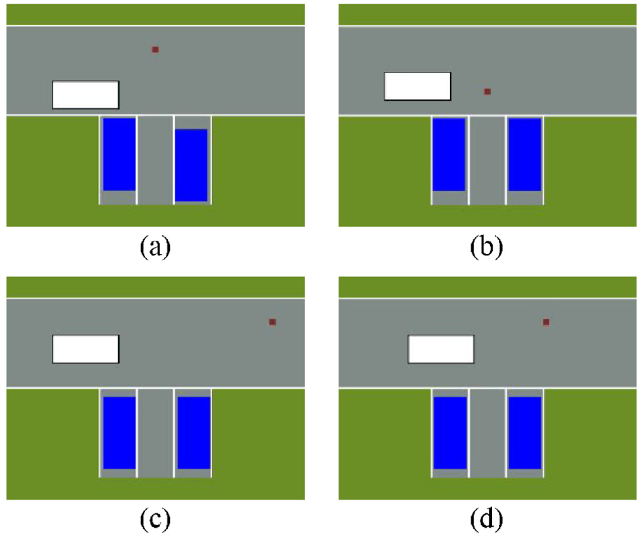
Schematic diagrams of test cases: (a) Test case T_1, (b) Test case T_2, (c) Test case T_3, and (d) Test case T_4.

It can be found from the schematic diagrams that the relative distances between objects in the T_2 is relatively small, while the relative distances between objects in the T_3 is relatively large, and their probability is small. In Table 9, the probability deviations of the two test cases are relatively small, the probabilities of the test cases are close to the expected probability $p_{e}^{g}$ , and the subjective judgments are consistent with the calculated values. The relative distances between the objects in the T_4 is moderate, which is a high probability situation and is consistent with the larger probability deviation in Table 9.

Number of test cases

As the number of test cases increases, the cost of completing the tests also increases. Therefore, the size of test case sets is also an important criterion for evaluating test case generation algorithms. When the target parameter p_e and the weight α both change from 0 to 1, the improved AETG algorithm and the CTBC algorithm are used to generate test cases in the test scenario with a smaller parameter space, and the sizes of the test case sets are shown in Figure 13.

Figure 13.

Number of the test cases in the test scenario with a smaller parameter space.

The number of optimal test cases is far exceeding the test case sets generated by the two algorithms, and the number fluctuates roughly around 60 due to the influence of target parameters. The size of the test case sets generated by the CTBC algorithm is smaller than the optimal test case sets, but slightly larger than the test case sets generated by the improved AETG algorithm. The number of the test cases fluctuates roughly around 30 affected by the target parameters. Compared with the target parameter, the sizes of the test case sets generated by the improved AETG algorithm is more sensitive to the weight.

Since the target parameter has little effect on the size of the test case set, we use the improved AETG algorithm and the CTBC algorithm to generate the test cases of the scenarios in Table 5 where p_e = 0.3 and α increase from 0 to 1, the sizes of the test case sets are shown in Figure 14.

Figure 14.

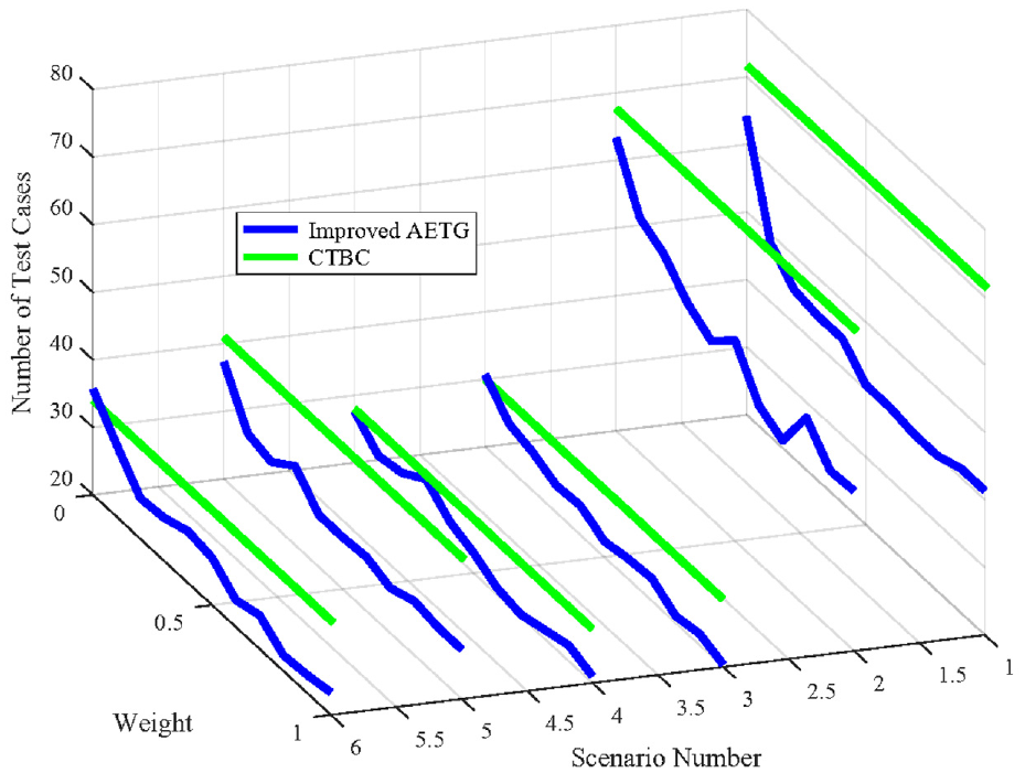
Number of the test cases in the sample scenarios (α = 0–1, p_e = 0.3).

The size of the test case set generated by the improved AETG algorithm is slightly smaller than of the CTBC algorithm, and the gap between the two test case sets gradually expends with the increase of weight. The parameter space and constraint set of each scenario are different, which leads to different sizes of test case sets.

Conclusion

Test scenario generation method is one of the key research directions of automated driving vehicle. In this paper, a test case generation algorithm for specific driving scenarios based on combinatorial testing and Bayesian network is proposed. When generating test cases, a group of test cases with different probabilities can be obtained by adjusting the weights and target parameters to meet the test tasks with different requirements.

By discretizing the continuous probability distribution, the conditional probability table of the scenario can be calculated by the relative parameters between the scenario objects. A composite selection function is formulated according to the probability and frequency of scenario cases. Then, the selection function is used as indicator to select the combination of parameter values when generating test cases.

Compared with the test case set generated by CTBC algorithm, the probability deviation of the test case set generated by the proposed improved AETG algorithm is smaller when the weight is less than 0.5, and the size of the test case set is smaller. The probability distribution of test cases is affected by their parameter space. In order to generate as many test cases with specific probability as possible, it is necessary to specially construct the parameter space of the test scenario.

This study focuses on the design of the test scenario generation method, but does not apply the scenarios to test autonomous vehicle. As the future work, an autonomous vehicle scenario simulation platform will be established, and the test efficiency of using the generated scenarios will be analyzed. Furthermore, we will establish the probability distribution functions based on real scenario data, considering the dynamic trajectory generation of objects and the interaction between multiple objects.

Footnotes

Declaration of conflicting interests

The author(s) declared no potential conflicts of interest with respect to the research, authorship, and/or publication of this article.

Funding

The author(s) disclosed receipt of the following financial support for the research, authorship, and/or publication of this article: This work was supported by the Anhui Science and Technology Key Special Program under [Grant No. 201903a05020016, 202004b11020002], Natural Science Foundation of Anhui Province [Grant No. 2208085QE153] and National Key R&D Program of China [Grant No. 2018YFB0105102]. The authors would like to thank the reviewers for their time and suggestions.

ORCID iDs

Xudong Hu

Bo Zhu

References

Koopman

Wagner

. Challenges in autonomous vehicle testing and validation. SAE Int J Transp Saf 2016; 4: 15–24.

Wachenfeld

Winner

. The release of autonomous vehicles. In: M

Maurer

Gerdes

Lenz

, et al. (eds) Autonomous driving: technical, legal and social aspects. Berlin, Heidelberg: Springer, 2016, pp.425–449.

Kalra

Paddock

. Driving to safety: How many miles of driving would it take to demonstrate autonomous vehicle reliability? Transp Res Part A Policy Pract 2016; 94: 182–193.

Menzel

Bagschik

Maurer

. Scenarios for development, test and validation of automated vehicles. In: 2018 IEEE intelligent vehicles symposium (IV), Changshu, China, 2018, pp.1821–1827. New York, NY: IEEE.

Junyou

Xuejian

Chai

. Design and realization of driving simulator system based on virtual reality. Mach Des Manuf 2013; 1: 39–41.

Huynh

Gambi

Fraser

. AC3R: Automatically reconstructing car crashes from police reports. In: 2019 IEEE/ACM 41st international conference on software engineering: companion proceedings (ICSE-Companion), Montreal, Canada, 2019, pp.31–34. New York, NY: IEEE.

Huang

Cheng

Geng

, et al. The ApolloScape dataset for autonomous driving. In: 2018 IEEE conference on computer vision and pattern recognition (CVPR), Salt Lake City, UT, 2018, pp.954–960. New York, NY: IEEE.

Medrano-Berumen

Akbas

. Abstract Simulation scenario generation for autonomous vehicle verification. In: IEEE Southeast conference, Huntsville, AL, 2019, pp.1–6. New York, NY: IEEE.

Shengshan

Jian

Jinsheng

, et al. Study on the reform of road driving skills test system. China Public Security 2019; 1: 117–120.

10.

Buechel

Hinz

Ruehl

, et al. Ontology-based traffic scene modeling, traffic regulations dependent situational awareness and decision-making for automated vehicles. In: 2017 IEEE intelligent vehicles symposium (IV), Los Angeles, CA, 2017, pp.1471–1476. New York, NY: IEEE.

11.

Cordts

Omran

Ramos

, et al. The Cityscapes dataset for semantic urban scene understanding. In: 2016 IEEE conference on computer vision and pattern recognition (CVPR), Las Vegas, NV, 2016, pp.3213–3223. New York, NY: IEEE.

12.

Geiger

Lenz

Urtasun

. Are we ready for autonomous driving? The KITTI vision benchmark suite. In: 2012 IEEE conference on computer vision and pattern recognition (CVPR), Providence, USA, 2012, pp.3354–3361. New York, NY: IEEE.

13.

Maddern

Pascoe

Linegar

, et al. 1 year, 1000 km: the Oxford RobotCar dataset. Int J Rob Res 2017; 36: 3–15.

14.

Xian

Chen

, et al. BDD100K: a diverse driving video database with scalable annotation tooling. In: 2020 IEEE conference on computer vision and pattern recognition (CVPR), Seattle, WA, 2018. New York, NY: IEEE.

15.

Rocklage

Kraft

Karatas

, et al. Automated scenario generation for regression testing of autonomous vehicles. In: 2017 IEEE 20th international conference on intelligent transportation systems (ITSC), Yokohama, Japan, 2017, pp.476–483. New York, NY: IEEE.

16.

Xia

Duan

Gao

, et al. Test scenario design for intelligent driving system ensuring coverage and effectiveness. Int J Autom Technol 2018; 19: 751–758.

17.

Khastgir

Dhadyalla

Birrell

, et al. Test scenario generation for driving simulators using constrained randomization technique. In: WCX17: SAE world congress experience, Detroit, MI, 2017. SAE International.

18.

Bing

Peixing

Jian

, et al. Review of scenario-based virtual validation methods for automated vehicles. China J Highw Transp 2019; 32: 1–19.

19.

Junzong

Chunnian

Zhiqiang

. Bayesian belief network model learning, inference and application. Comput Eng Appl 2003; 1: 24–27.

20.

Zhao

Lam

Peng

, et al. Accelerated Evaluation of Automated Vehicles Safety in Lane-change scenarios based on importance sampling techniques. IEEE Trans Intell Transp Syst 2017; 18: 595–607.

21.

Duan

Lei

, et al. Constraint handling in combinatorial test generation using forbidden tuples. In: IEEE international conference on software testing, verification and validation workshops (ICSTW), Graz, Austria, 2015, pp.1–9. New York, NY: IEEE.

22.

Mengfan

. Constraints in combinational testing. Nanjing: Nanjing University, 2017.

23.

Cui

Yang

. Combinatorial test cases with constraints in software systems. In: IEEE 16th international conference on computer supported cooperative work in design (CSCWD), Wuhan, China, 2012, pp.195–199. New York, NY: IEEE.

24.

Wang

. The driving safety field based on driver–vehicle–road interactions. IEEE Trans Intell Transp Syst 2015; 16: 2203–2214.

25.

Wang

Zheng

, et al. Driving safety field theory modeling and its application in pre-collision warning system. Transp Res Part C Emerg Technol 2016; 72: 306–324.

26.

Chen

Sherony

Gabler

. Comparison of time to collision and enhanced time to collision at brake application during normal driving. In: SAE 2016 world congress and exhibition 2016.

27.

Feng

, et al. Testing Scenario Library Generation for connected and automated vehicles, Part I: methodology. IEEE Trans Intell Transp Syst 2021; 22: 1573–1582.

28.

Haitao

Qiuyue

. The optimal solution of the reordering newsboy problem with triangular demand distribution. J Inner Mongolia Univ Nationalities 2003; 1: 289–292.

29.

Fan

Xiaoqiu

. Method of Generation Pair-cover test cases based on AETG algorithm. Comput Eng Des 2014; 35: 3850–3854.

30.

Zhenyu

Jun

. Research on priority-based combinatorial testing method. Comput Digit Eng 2012; 40: 85–87.

31.

Xiaoying

Jun

. Case generation by constraints combinatorial testing. J Tsinghua Univ (Sci Technol) 2017; 57: 225–233.

32.

Kuhn

Reilly

. An investigation of the applicability of design of experiments to software testing. In: 27th Annual NASA Goddard/IEEE software engineering workshop, Greenbelt, MD, 2002, pp.91–95. New York, NY: IEEE.

33.

Kuhn

Kacker

Lei

, et al. Combinatorial software testing. Computer 2009; 42: 94–96.

34.

Duan

Gao

. Test scenario generation and optimization technology for intelligent driving systems. IEEE Intell Transp Syst Mag 2022; 14: 115–127.

Test scenario generation method for autonomous vehicles based on combinatorial testing and Bayesian network

Abstract

Keywords

Introduction

Parameters of test scenario

Environment

Road

Object

Type of scenario

Constraints in test scenario

Initial constraint set

Implied forbidden tuple

Construction of Bayesian network

Structure of Bayesian network

Conditional probability

Scenario generation algorithm

Uncovered combination set

Selection function

Test case generation

Result of scenario generation

Probability deviation

Number of test cases

Conclusion

Footnotes

Declaration of conflicting interests

Funding

ORCID iDs

References