
Abstract
This paper proposes tools from bifurcation theory, specifically numerical continuation, as a complementary method for efficiently mapping the state-parameter space of an internal combustion engine model. Numerical continuation allows a steady-state engine response to be traced directly through the state-parameter space, under the simultaneous variation of one or more model parameters. By applying this approach to two nonlinear engine models (a physics-based model and a data-driven model), this work determines how input parameters ‘throttle position’ and ‘desired load torque’ affect the engine’s dynamics. Performing a bifurcation analysis allows the model’s parameter space to be divided into regions of different qualitative types of the dynamic behaviour, with the identified bifurcations shown to correspond to key physical properties of the system in the physics-based model: minimum throttle angles required for steady-state operation of the engine are indicated by fold bifurcations; regions containing self-sustaining oscillations are bounded by supercritical Hopf bifurcations. The bifurcation analysis of a data-driven engine model shows how numerical continuation could be used to evaluate the efficacy of data-driven models.
Introduction
Engineers often make use of computer models to replicate dynamic behaviour. When nonlinearities are known to influence model output, time history simulations can be used to build up a picture of a given model’s dynamic behaviour by running multiple simulations for different initial conditions, to identify (for example) which inputs produce a given output. While a simulation of a computation model for one initial condition and one set of parameters can be a relatively short process, the cumulative time needed to simulate the response for many different initial conditions and parameter values means that time history simulations can become computationally inefficient. If the system’s steady-state is of interest (such as in traditional engine mapping), transient behaviour needs to be simulated first as the system reaches a steady-state: this adds time to each simulation.
The presence and location of any repelling equilibria are also difficult to find through conventional time history simulations alone, because initial conditions that start near repelling equilibria move away from these equilibria over time. Although real systems do not reach repelling equilibria, knowledge of their location allows engineers to identify key regions in the system’s state space, as they often separate regions of the state space where similar initial conditions may have quite different steady-state responses.
A variety of approaches to complement conventional time history simulations of nonlinear dynamic models have been presented in engine literature: recurrence plots and recurrence quantification analysis have been used to investigate the relation between injection impulse with engine speed 1 and the dynamics associated with cycle-to-cycle variations in a diesel engine 2 ; multi-level substructuring procedures were used to study periodic responses of large engine models in Theodosiou et al. 3 ; 0-1 testing was applied to classify chaotic behaviour within the combustion process. 4 Understanding the steady-state response of engine models is also highlighted as a challenge in the literature: in Beno et al., 5 the authors studied the calibration of a turbocharged diesel engine by representing the highly nonlinear system as a mean value model. All of these approaches serve to enhance the automotive engineer’s toolbox of analysis techniques, allowing specific information from a dynamic model to be obtained efficiently. For example, these studies were useful in obtaining useful information about the combustion process in specific cases, revealing that it becomes highly sensitive to initial conditions under certain conditions: reducing engine speed and torque to low values presents chaotic behaviour, while raising speed and torque to high values removes this behaviour.
A bifurcation analysis approach is an alternative method of obtaining useful information about a nonlinear system’s dynamics. Bifurcation theory considers how the equilibrium solutions of system of ordinary differential equations change as one or more parameter is varied. When the equilibrium solution experiences a qualitative change in behaviour, such as a change in stability, it is said to bifurcate: these points have particular mathematical descriptions, and can be followed under the simultaneous variation of multiple parameters. Bifurcation theory has been previously used to help understand a variety of dynamics problems in the engineering industry, seeing extensive use in aeronautical literature: bifurcation analysis has been shown to be a useful tool in studying aeroelasticity in wings, observing self-sustaining oscillations under the variation of one or more parameters6,7; it has been used in the analysis of aircraft undertaking ground manoeuvres8–10 and also the analysis and recovery of deep stall. 11 The approach obtains results that would be unobtainable with linear analysis alone.
The approach has also been used in current literature directly related to the automotive industry, in areas such as vehicle dynamics, wheel and suspension dynamics, permanent synchronous motors and braking systems. A bifurcation analysis helped determine how driving speed and steering angle 12 and torque and steering angle 13 affect the stability in a cornering vehicle. In addition, the lateral dynamics of a vehicle driving straight ahead was also studied. 14 The methods are also shown to be useful in the analysis of wheels, tyres and suspension dynamics, with the damping force shown to dramatically affect the behaviour of the suspension 15 and the slip angle and vehicle speed shown to play major roles in the development of vibration. 14 Shimmy behaviour has also been studied, with limit cycles being observed under bisectional road conditions 16 and bistable parameter ranges were found for towed wheels. 17 Furthermore, the approach was used in determining the stability of permanent synchronous motors 18 and regions of dynamic behaviour in braking dynamics. 19 More generally, the approach has been used to study larger vehicles, including how lane changes effect buses 20 and semi-trailers 21 and finding critical speeds for railway vehicles. 22
Bifurcation analysis is proposed in this work as another complementary approach that can be used to explore the nonlinear dynamic behaviour of engines. To perform a bifurcation analysis on systems (such as engines) where the dynamic equations do not yield analytical expressions for their bifurcations, numerical continuation is the method used to undertake a computational bifurcation study. Starting from a known steady-state response, the numerical continuation algorithm traces out branches of equilibria under the variation of one parameter. When a bifurcation is detected, the continuation algorithm can trace out branches of the same type of bifurcation as two parameters are varied (simultaneously). The branches of equilibria and bifurcations are usually displayed on bifurcation diagrams, which illustrate the long-term behaviour of the nonlinear dynamic system. For further information on bifurcation theory, see Strogatz 23 and Yuznetsov. 24
While previous applications of bifurcation theory are broad, to the authors’ knowledge, bifurcation analysis methods have seen limited application to the study of engine dynamics. The authors have previously presented a bifurcation analysis of an open-loop internal combustion engine 25 where two parameters, throttle and torque, have been varied. This paper expands on the previous work by conducting additional two-parameter and new three-parameter continuations, including a more realistic altitude and temperature model and the analysis of a data-driven model. To the authors’ knowledge, these are the first examples of papers to conduct a full bifurcation analysis of an open-loop internal combustion engine of both a data-driven and physics-based model.
The aim of this paper is to demonstrate how a bifurcation analysis can be used to complement conventional time history simulations in the analysis of internal combustion engine models. The numerical continuation code AUTO,26–28 integrated into MATLAB via the dynamical systems toolbox, 29 is used to conduct the bifurcation analysis. The paper begins with an overview of two models used in the paper: one physics-based model and one data-driven model. The physics-based model is studied first, to demonstrate how the approach can be used to provide insight into engine dynamics for different operating points of throttle and desired load torque. The sensitivity of this behaviour to changes in additional parameters is then studied, before comparing the bifurcation results from the physics-based model with results from a data-driven model. This demonstrates the application of numerical continuation to more robust and realistic engine model. Finally, key findings from the analysis of both models are compared and summarized, and recommendations for future work are outlined.
Engine models
This work uses two different model types: a physics-based model adapted from Guzzella and Onder 30 and a data-driven model, created from engine test data. These two models are used to demonstrate the applicability of bifurcation analysis methods to the study of engine dynamics, given that engine models may be physics-based, data-driven or a combination of the two.
Physics-based engine model
The following assumptions, as described by Guzzella and Onder, 30 are made in the derivation of this model:
Throttle area;
The dynamics of the actuator may be neglected
Throttle mass flow;
Air is a perfect gas, throttle is isenthalpic
Air mass sensor;
Sensor is a static linear system with known characteristics
Intake manifold;
Lumped-parameter model, isothermal conditions.
Pressure sensor;
Sensor is a static linear system.
Engine mass-flow;
No pressure drop in the intake runners.
The temperature drop from the evaporation of the fuel is cancelled out by the heating effect of the hot intake duct walls.
The temperature in the cylinder is thus the same as in the intake manifold.
The air/fuel ratio is constant and equal to stoichiometry.
Volumetric efficiency depends on manifold pressure
The exhaust manifold pressure is constant.
Torque generation;
The engine may be simplified as a Willans machine
The calculation time and the sampling time can be neglected.
Engine inertia;
The engine has a constant inertia and all internal friction is included (in the input).
Engine-speed sensor;
The sensor is linear and very fast.
Load Torque;
The dynamics of the alternator and electronic load may be lumped into one first-order system. 30
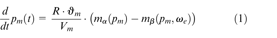
The physics-based model is governed by three coupled first-order nonlinear differential equations. The dynamics associated with the intake manifold pressure,
Here,
Equation (1) is the first differential equation and models the dynamics associated with the mass flow entering
Here,
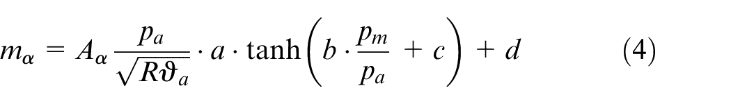
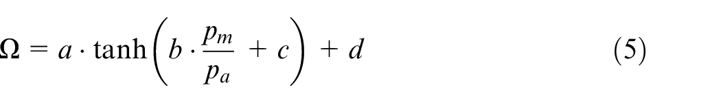
To conduct a bifurcation analysis, all equations must be smooth. Therefore, rather than use a piecewise approximation as in Guzzella and Onder,
30
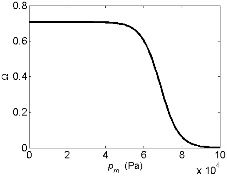
the values of a, b, c and d are chosen to provide a physically reasonable approximation of the throttle mass flow. Figure 1 demonstrates the output of the fitted curve in equation (5) as a function of
The throttle area,
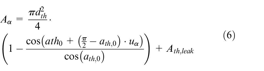
Here,
The mass flow exiting the manifold is modelled by equation (7) 30
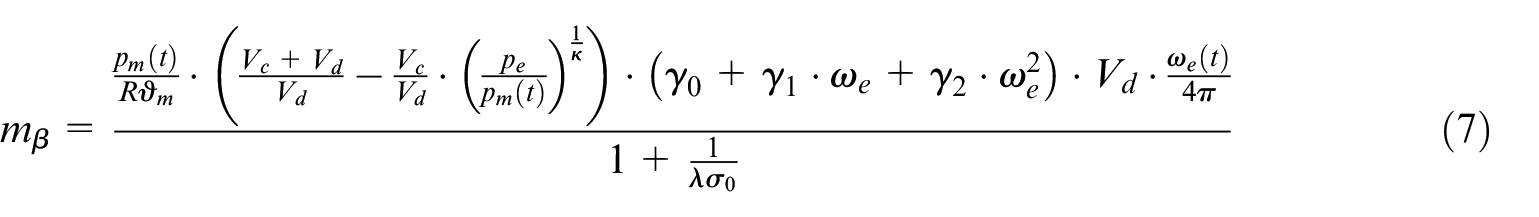
Here,
An approximation of the physics in the mass flow equation (4). For
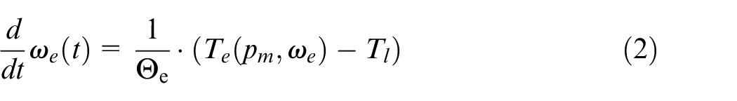
The second differential equation (equation (2)) models the dynamics associated with the engine’s rotational motion, which depends on the engine’s capacity to generate torque. The torque generated by the engine

Here, the terms
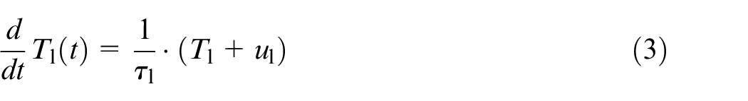
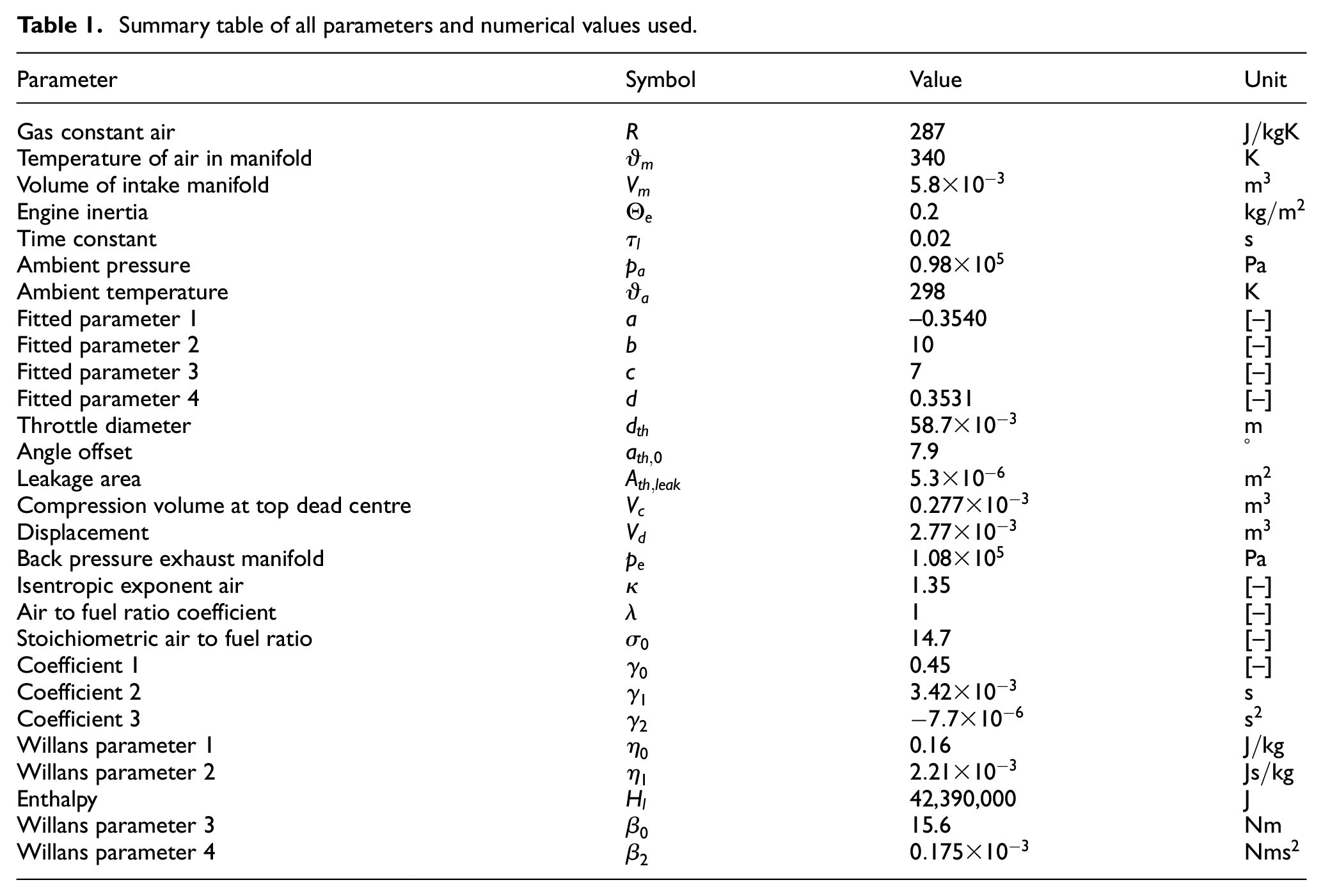
Equation (3) is the final differential equation, which models the load torque as a first-order delay. The numerical values used are summarized in Table 1.
Summary table of all parameters and numerical values used.
Data-driven engine model
Engine models used in industrial settings often make use of experimental data to generate a dynamic model. For bifurcation methods to be appropriate for an industrial context, they need to be shown to work for these sorts of data-driven models. In this work, a data-driven engine model taken from MathWorks 31 is studied, to show that bifurcation methods can be used to analyse data-driven models as well as equation-based physics models.
Figure 2 provides a schematic of the data-driven Simulink model used. The top-level model has two inputs: a transmission torque (in Nm) and a throttle position (expressed as a percentage). The ‘EngineTorque’ block in Figure 2 is a two-dimensional data table that relates a throttle position and engine speed input to an engine torque output. The input ‘Transmission_Torque’ represents the external load applied to the engine, which may arise in real operations due to road gradients, drag or rolling resistance. The difference between this externally applied torque and the torque produced by the engine causes the engine to speed up or slow down: the engine speed is determined by dividing the net torque using a representative inertia value (‘EnginePlusImpellerInertia’) to obtain the engine’s acceleration, and then integrating acceleration to calculate engine speed (Ne). Although this is a simplistic model, the data table captures a typical nonlinear relation between engine speed and the torque that is produced (both as a function of throttle position). A visual representation of the data table contained in the model is shown in Figure 3. The model assumes that the data collected is sufficient to capture the relation between throttle position, engine speed and engine torque.
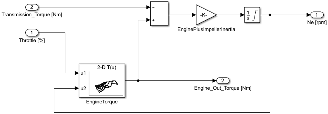
A schematic view of the data-driven model.
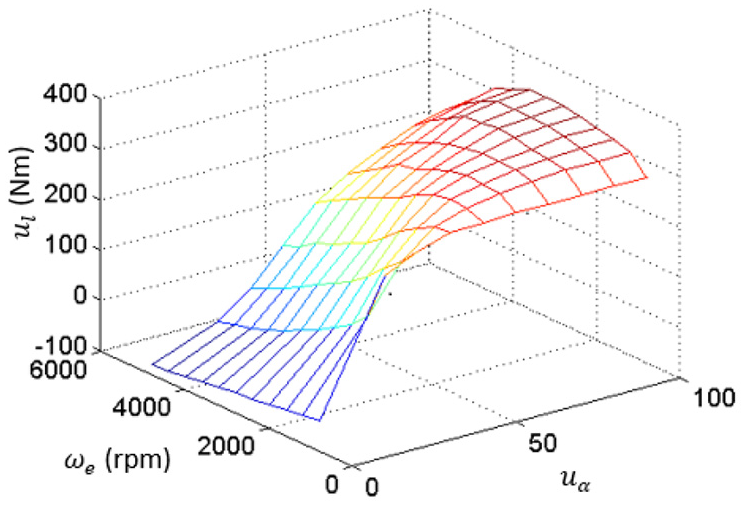
The raw data collected from the test bed. Inputs throttle and engine speed are related to a torque value.
The above data provide an accurate torque output based on engine speed and throttle angle. The discontinuous nature of such data, shown in Figure 3, makes a bifurcation analysis of the system in its current form infeasible. As such, the data need to be smoothed with an appropriate interpolation and extrapolation method. Simulink offers several techniques to smooth the data for interpolation and extrapolation purposes: in this study, the inbuilt cubic spline technique is used to fit a continuous third-order polynomial through neighbouring data points in the ‘EngineTorque’ data block. This ensures data are as smooth as possible for the nonlinear analysis.
Figure 4 provides time history simulations at an example operating point
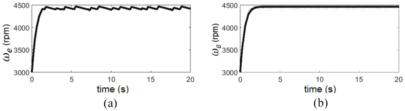
Two time history simulations at a given operating point for the unsmooth data (a) and smoothed data (b).
Bifurcation analysis of physics-based engine model
This section contains a demonstration of a bifurcation analysis of the physics-based model and a discussion of the results obtained at each stage. To begin, one parameter will be varied to show the different types of bifurcation that exist in the state-parameter space. With the bifurcations observed, these points themselves can then be traced in a two-parameter continuation, showing any complexities or additional bifurcations that exist under the variation of two parameters. These results exhibit dynamics first presented by the authors in Smith et al., 25 but they provide relevant context in this paper for the subsequent sensitivity study and comparison with results from a data-driven engine model. The sensitivity study shows how the nonlinear dynamic behaviour changes as a third parameter of operational interest is varied, expanding on previous results in Smith et al., 25 by constructing surfaces of bifurcations to show their quantitative variation as a function of three parameters of interest. The analysis also expands on previous work through inclusion of new results showing how peak engine torque varies with these additional parameters.
One-parameter continuation results
Throttle angle,
Each bifurcation diagram may contain several branches of equilibria and type of bifurcation. All are described in detail as and when they occur; however, a summary is also provided in Table 2.
Summary table of all definitions to aid reading of bifurcation diagram in order of appearance.
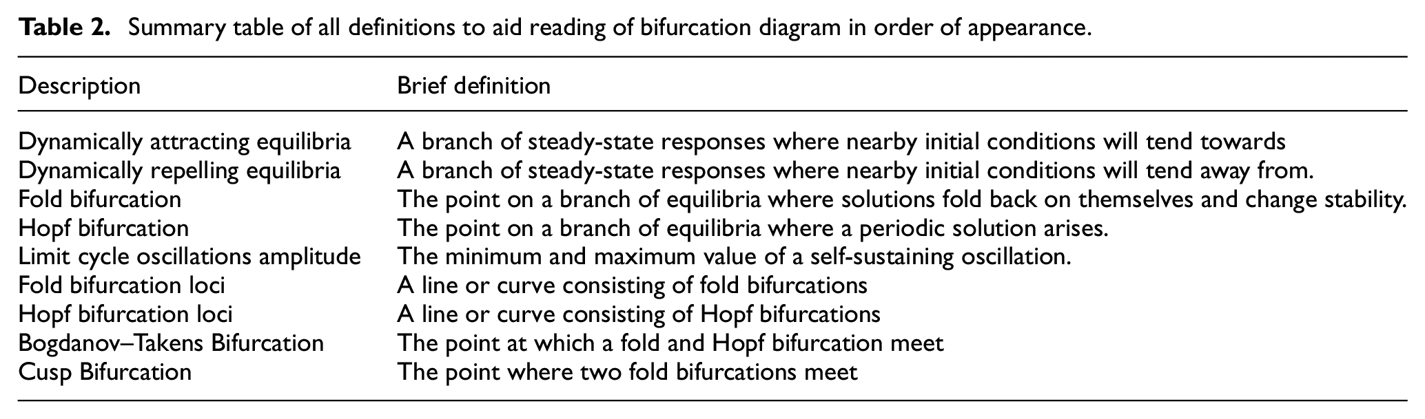
Figure 5 shows the first bifurcation diagram which shows the steady-state engine response of both manifold pressure (a) and engine speed (b) as a function of
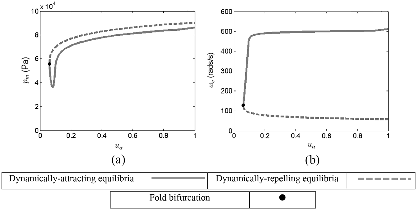
One-parameter bifurcation diagram for a fixed load torque
As throttle angle is increased, the steady-state engine speed achieved at the attracting equilibria (solid curve, Figure 5(b)) increases rapidly over a narrow range of throttle angles from
The concept of a repelling equilibrium point is less intuitive, because systems at such points are unstable – they are hence seldom observed directly in real systems. An intuitive example of a repelling equilibrium point in a physical system is an ‘upside-down’ rigid pendulum: mathematically, such a condition exists, but in practice, the pendulum would fall from this position if disturbed even slightly and end up hanging down (at the attracting equilibrium position). Because of their nature, repelling equilibria are difficult to observe through conventional time history simulations, but they are important for the dynamics of the system because they separate nearby initial conditions that lead to different long-term behaviour: in the case of the pendulum, the repelling equilibrium point dictates if initial conditions (value at t = 0 for angular position and angular velocity) will result in the pendulum swinging clockwise or anti-clockwise; for the engine, the repelling equilibria dictate if the initial condition (value at t = 0 for manifold pressure and engine speed) will cause engine speed to increase or decrease.
For values of
Piecing the information together from the description of the bifurcation diagram, it can be shown that the bifurcation diagram enables the destination of any dynamic trajectory to be inferred, that is, work out where the system will end up as
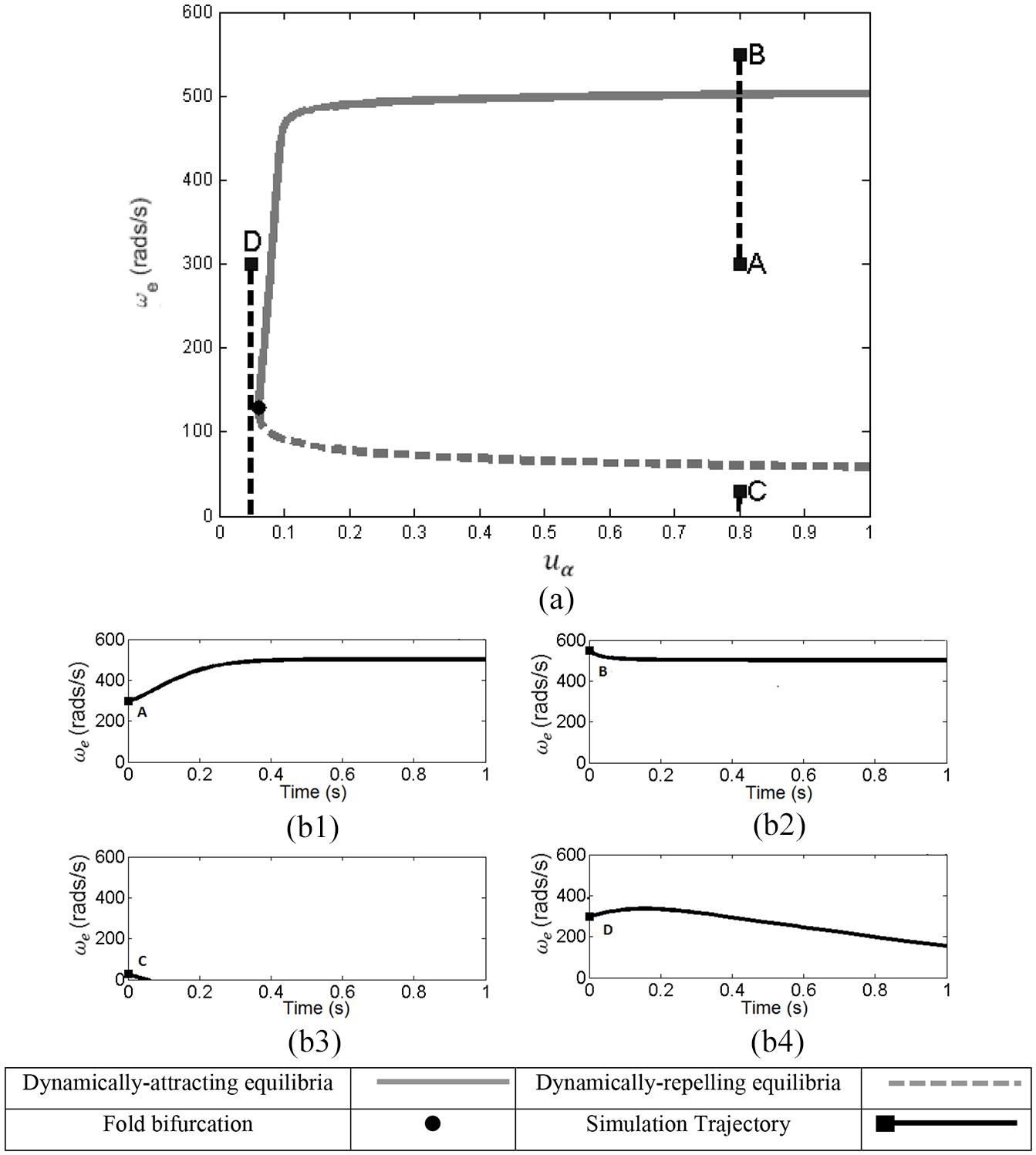
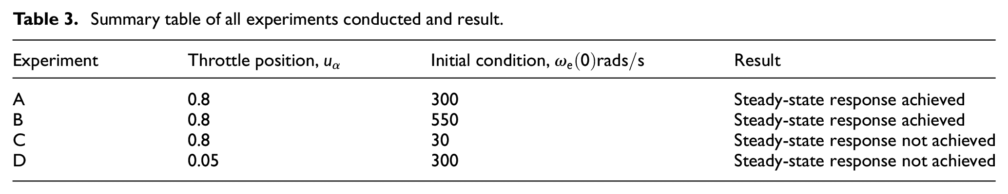
Four example initial conditions (A, B, C and D) are shown on the bifurcation diagram (a) and in a time history simulation (b1–b4). Trajectories either arrive at the stable branch, and therefore achieve a steady-state response, or tend towards zero and do not reach this.
Summary table of all experiments conducted and result.
The bifurcation diagrams in Figures 5 and 6 were obtained for one specific engine load,
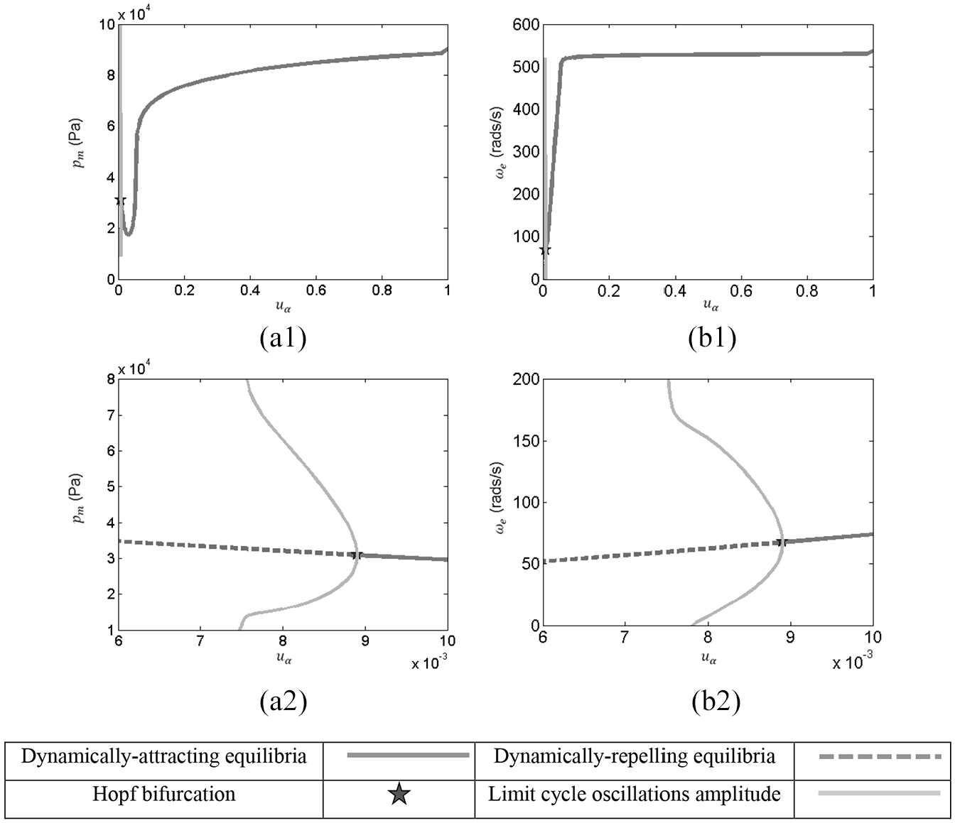
One-parameter bifurcation diagram showing the response of (a1) manifold pressure and (b1) engine speed (with zoomed view (a2) and (b2) below) for
To demonstrate that this periodic behaviour is a function of the mathematical model, Figure 8 contains the dynamic response either side of the Hopf bifurcation. Figure 8(a) and (b) shows the response for
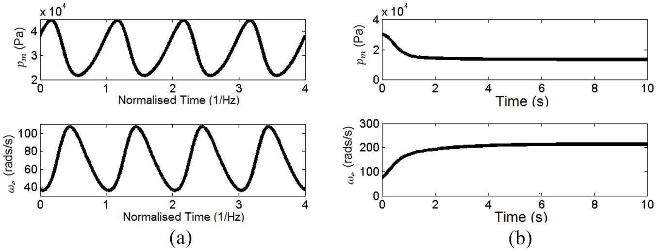
A time history simulation for
A possible explanation for the occurrence of a Hopf bifurcation in the model at low load is that the engine speeds up too much for the amount of air that can be drawn into the cylinders. When the throttle angle is slightly open (e.g. Figure 8(a)), there is enough airflow to increase the engine’s speed; however, the momentum gained causes the engine speed to rise to a point at which it cannot be sustained with this throttle angle. At peak engine speed, the air flowing into the cylinder is insufficient to sustain the peak speed, so the engine slows down. During the deceleration, the airflow again becomes sufficient to drive the engine at a given speed; however, the inertia causes the engine to continue to decelerate past this sustainable level to a minimum speed. At this minimum speed, the engine can get sufficient air to sustain a higher speed, so it accelerates, and the process repeats indefinitely. This out-of-phase motion between pressure and speed is observable in Figure 8(a). Figure 8(b) shows a time history simulation at a throttle angle just above the Hopf bifurcation
The one-parameter bifurcation diagrams in Figures 6 and 7 have shown that the engine model exhibits different dynamic behaviours at different loads. The following section presents a two-parameter bifurcation analysis of the engine in order to study how the engine’s dynamics vary with different load conditions.
Two-parameter continuation results
The evolution of the fold and Hopf bifurcations can be numerically traced throughout the model’s state-parameter space as both throttle angle and load torque are varied simultaneously. Computations of this kind are defined as two-parameter continuations: they provide further information about the location of each bifurcation and any interactions between the two.
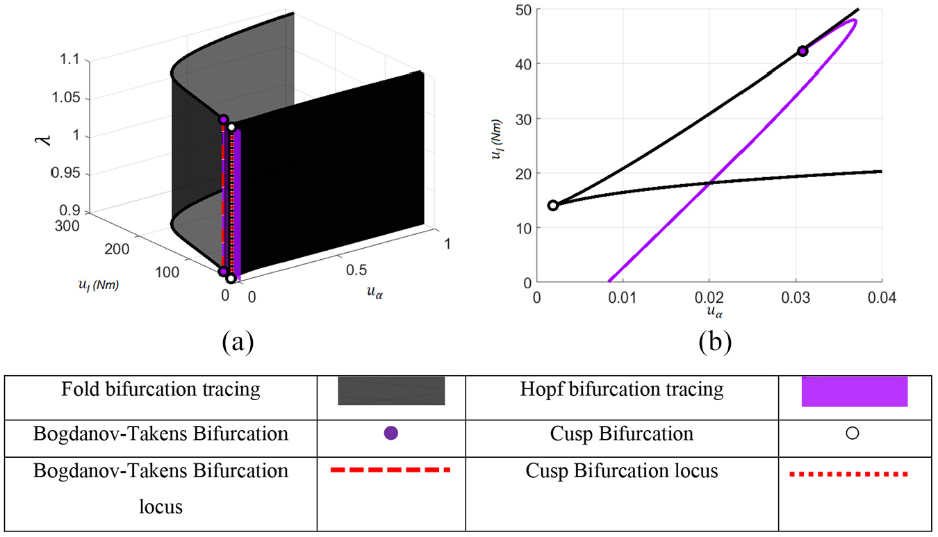
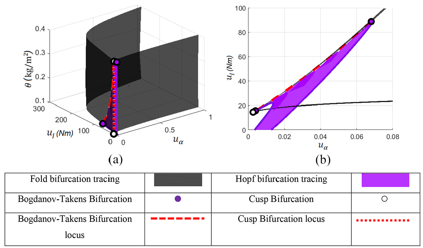
Figure 9 presents the results of the two-parameter continuation and shows the evolution of fold and Hopf loci. There are several features of the graph produced. The fold locus turns back on itself, and the point at which this occurs is known as a cusp bifurcation. The Hopf locus also turns back on itself and then collides with the fold locus: the exact point where the loci collide is called a Bogdanov–Takens bifurcation and terminates the locus of Hopf points.
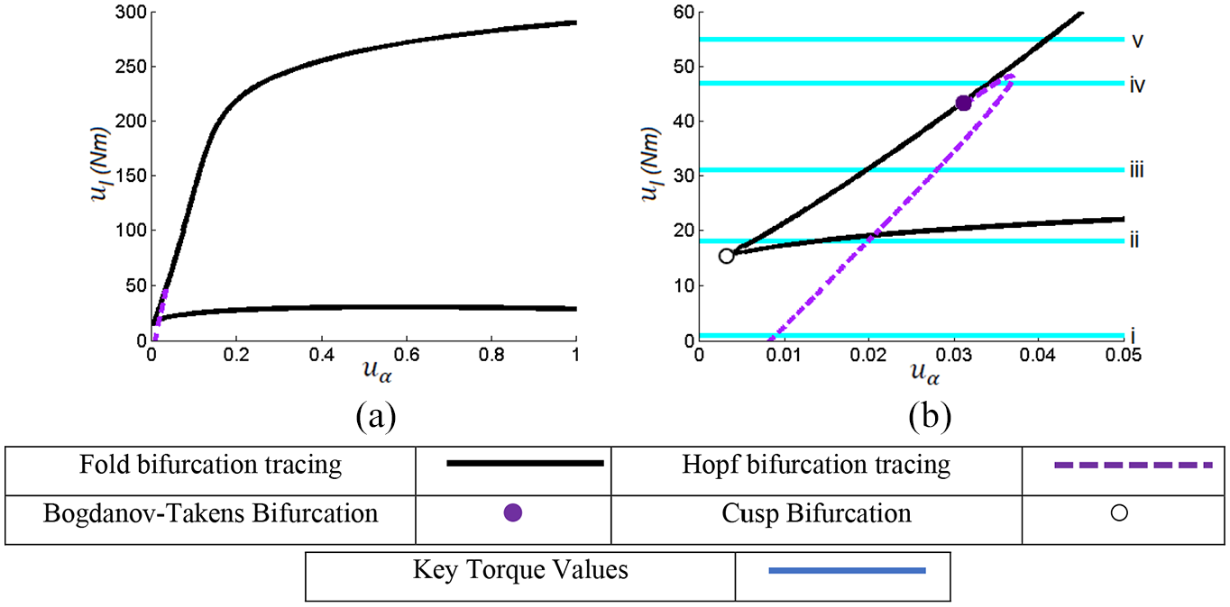
Two-parameter continuation of the fold and Hopf bifurcation points for (a)
At high torque values, there is only a fold bifurcation, indicating a one-parameter continuation in this region as in Figure 5. At lower torque values, only Hopf bifurcation exists, meaning one-parameter continuations here will result in figures such as that in Figure 7.
In the region between the two load cases already considered, as the curves turn back on themselves, one-parameter continuations could contain multiple fold and Hopf bifurcations depending on the corresponding torque values. To demonstrate the behaviour that exists in this region, one-parameter continuation diagrams can be created at appropriate torque values. Figure 9(b) also contains markings at five key torque values, cases (i)–(v). Case (i) is the value already considered in Figure 5 and is representative of the behaviour from
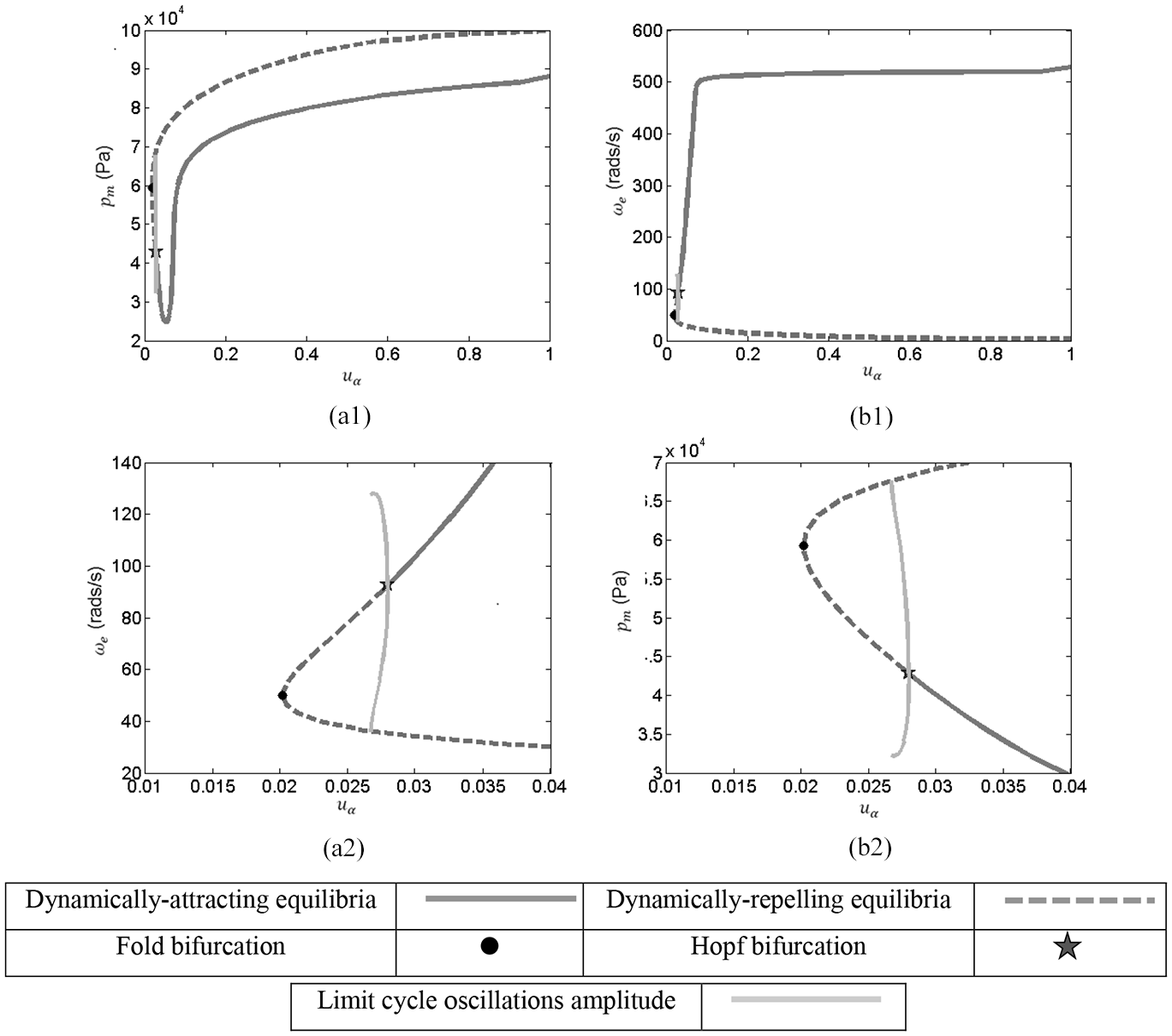
The torque value in case (ii) corresponds to a torque value immediately above the cusp bifurcation. The resulting one-parameter bifurcation diagram can be found in Figure 10. Increasing the load torque beyond the value at the cusp point results is a branch of dynamically attracting and repelling equilibria separated by a Hopf bifurcation, with two further fold bifurcations on the repelling branch. The amplitudes of the Hopf bifurcation grow until they collide with the repelling branch, which has changed location due to the fold loci. The resulting collision creates a homoclinic orbit. For throttle angles to the left of the homoclinic orbit, there is only repelling equilibria with no periodic behaviour. Any time history simulation in this region would head towards a zero-engine speed. Throttle angles above the Hopf bifurcation result in a steady-state engine response being achievable. Between the Hopf bifurcation and the homoclinic orbit is the region in which periodic responses occur. A possible explanation for this behaviour is that unlike Figures 7 and 8, there is an extra region of behaviour where, for higher torques at low throttle angles, not enough air can get through to maintain any level of engine speed. For the long-term response to be steady state, the mass flow in must be greater than the mass flow out, that is,
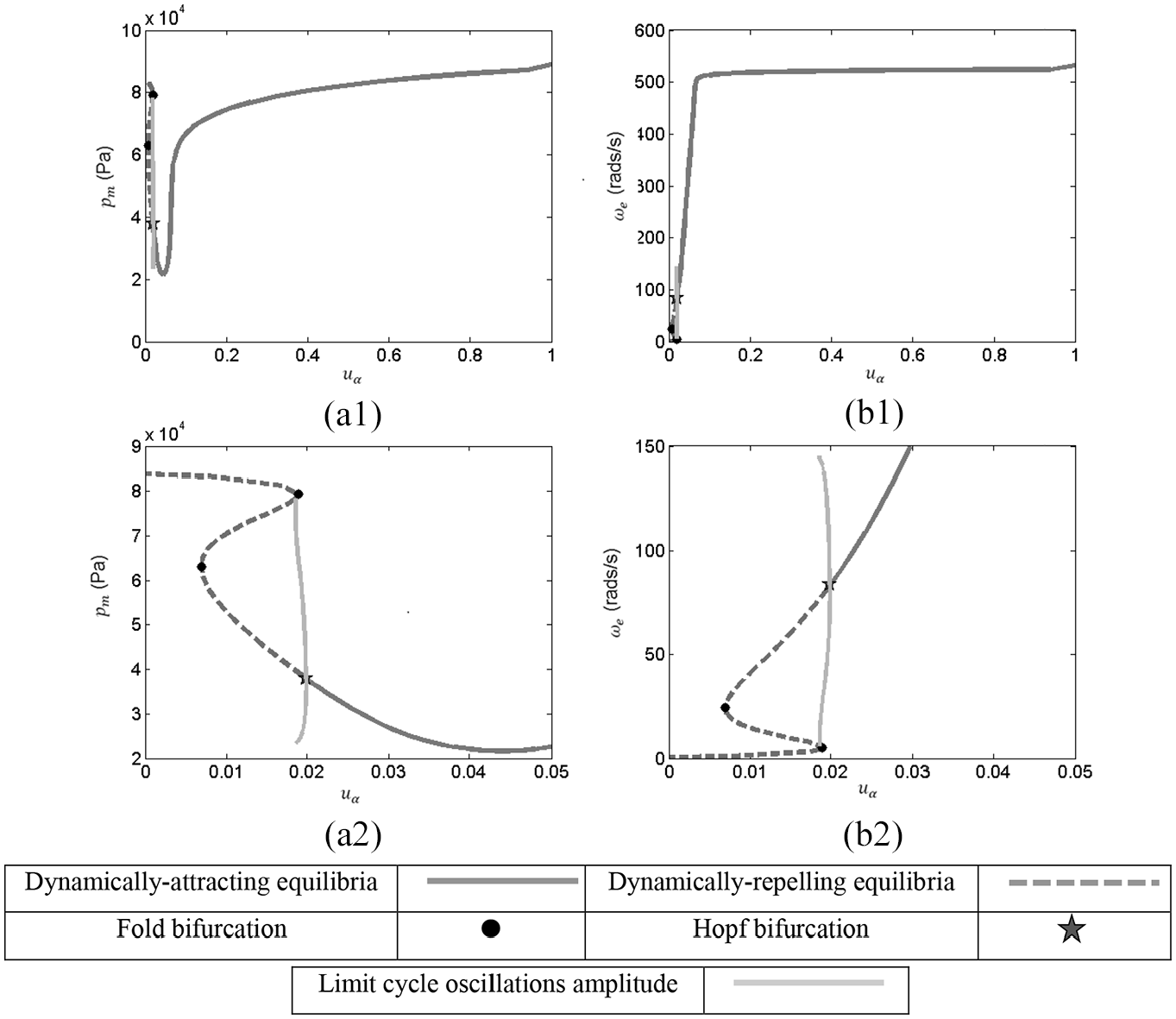
One-parameter bifurcation diagram showing the response of (a1) manifold pressure and (b1) engine speed (with zoomed view (a2) and (b2) below) for
For a higher torque value, both fold bifurcations move position until one leaves the physically meaningful range. Figure 11 contains the one-parameter bifurcation for case (iii) which is an example of a curve featuring a single fold and Hopf bifurcation. As before, there is a homoclinic orbit; however, as the second fold has left the physically meaningful region, no equilibria exist for very low throttle angles.
One-parameter bifurcation diagram showing the response of (a1) manifold pressure and (b1) engine speed (with zoomed view (a2) and (b2) below) for
Raising the torque allows the effects of case (iv) to be demonstrated. At this point, the torque is above the Bogdanov–Takens bifurcation, but not high enough to surpass the point at which the Hopf loci turns back on itself. This case is therefore unique as two Hopf bifurcations will exist in this region. Figure 12 contains a bifurcation diagram for the one-parameter continuation at 47Nm showing these two Hopf bifurcations which bound the limit cycle region. Increasing torque to a higher value means these Hopf bifurcations will get closer to each other and the size of the amplitudes of the limit cycles’ oscitations will shrink until the two Hopf bifurcations collide and are destroyed.
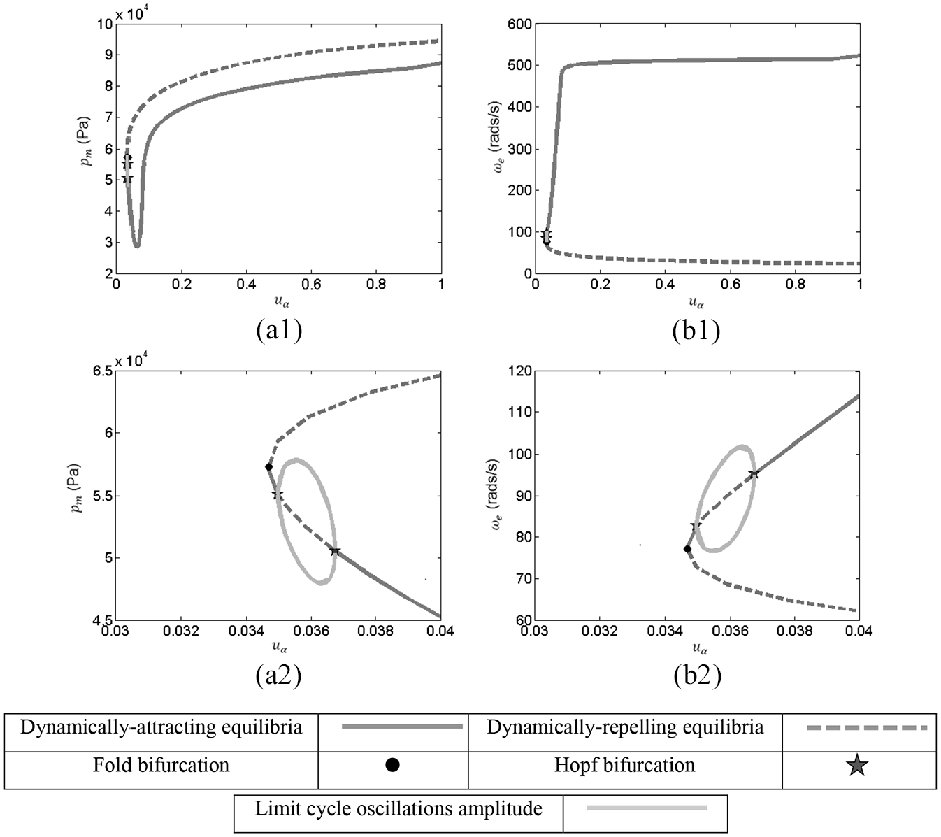
One-parameter bifurcation diagram showing the response of (a1) manifold pressure and (b1) engine speed (with zoomed view (a2) and (b2) below) for
Case (v) is shown in Figure 13 and is representative when torque is raised to 55Nm. The system returns to a structure that is equivalent to the structure shown in Figure 5. This qualitative description is the same for remaining torque values until the peak load torque of 282Nm which is the point at which the minimum throttle angle (denoted by the fold bifurcation) leaves the physical meaningful range
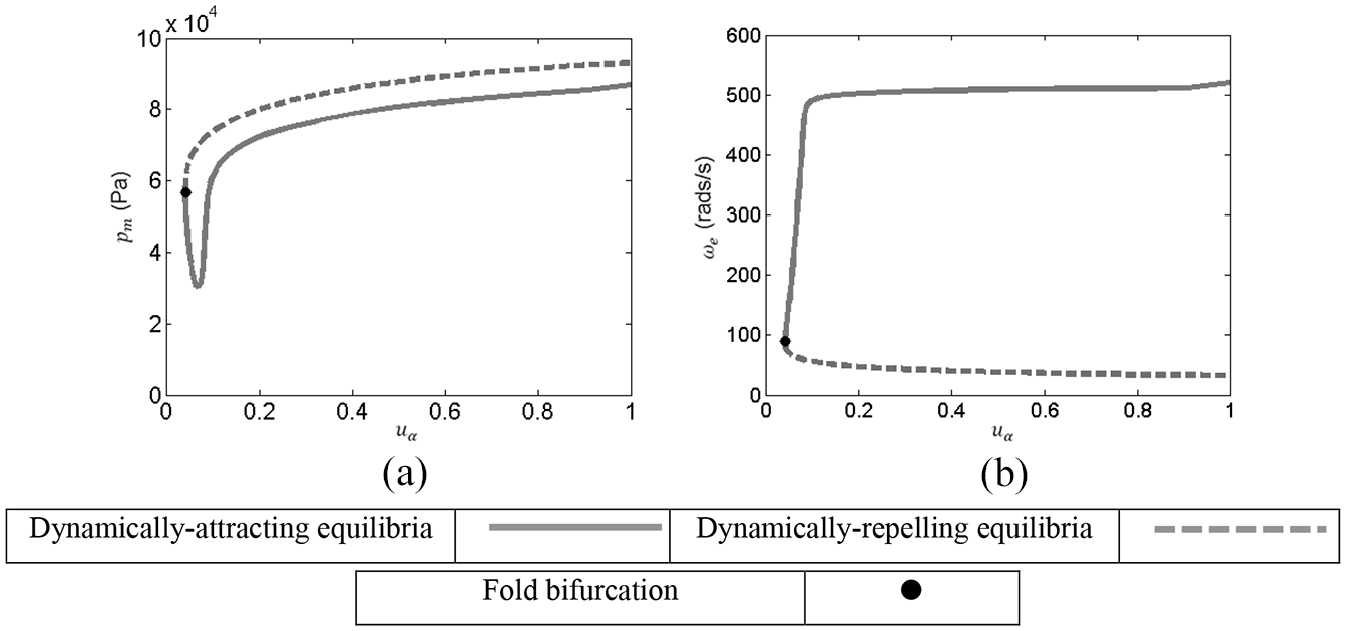
One-parameter bifurcation diagram showing the response of (a) manifold pressure and (b) engine speed for
Figures 10–13 contain branches of dynamically attracting equilibria that have a similar structure. Using traditional time history simulations alone, the detection of the dynamically repelling equilibria would have been much more difficult to observe and required an extensive number of simulations for a range of initial conditions and parameter values. In addition, the region of limit cycle oscillations is very small, making it difficult to find using time history simulations alone.
With the two-parameter bifurcation diagram describing the engine’s dynamics in terms of engine speed and load, it is possible to investigate how this picture changes as other parameters are altered. The subsequent section preforms a sensitivity analysis of the results obtained so far, to further demonstrate the usefulness of a bifurcation approach.
Sensitivity analysis of the bifurcation diagrams
The previous bifurcation analyses present an overview of all the bifurcations in the system’s state-parameter space and the type of behaviour to be expected. In this section, the preceding results will be treated as a benchmark case, and the sensitivity of the bifurcations to changes in additional model parameters values is investigated. By varying throttle, torque and a third parameter, a three-dimensional (3D) bifurcation diagram can be constructed by stacking multiple two-parameter continuation results and plotting the results as a surface in terms of the three parameters. These results can be compared to the benchmark case to determine how sensitive these bifurcations are to change in these additional parameters.
In the model, a controller is assumed to fix the air–fuel ratio
A bifurcation diagram with three-parameters, showing (a) the evolution of the bifurcations as
Another constant in the model is ambient pressure which is fixed to
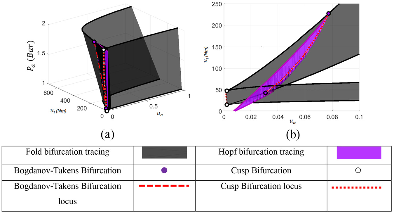
A bifurcation diagram with three-parameters, showing (a) the evolution of the bifurcations as ambient pressure is increased from 1 to 2 and (b) a zoomed view in the load–throttle plane.
Additional continuations can verify this result and also determine whether the relationship between peak load torque and the alteration we wish to make, in this case a change in pressure, is nonlinear. By fixing throttle angle to its maximum value and tracing the fold bifurcation as torque varies with ambient pressure provides the peak load torque value for across the parameter range. Figure 16 shows the exact peak load torque available as ambient pressure is varied across the
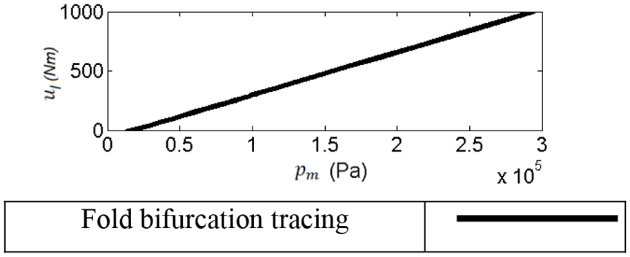
Two-parameter continuation showing how peak load torque varies as ambient pressure increases.
In order to simulate changes to altitude, ambient pressure
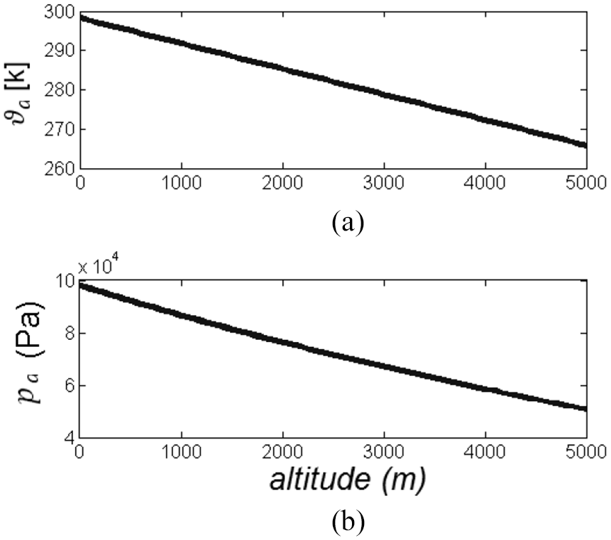
Ambient temperature
Conversely, decreasing ambient pressure, along with decreasing the ambient temperature, replicates the effects of running the engine at altitude. Figure 18 provides the results for two continuations when parameters are changed to replicate what they would be in extreme conditions such as an altitude up to 4000 m. In comparison to Figure 15, the changes are reversed: as a higher altitude limits the amount of the airflow into the system, the fold locus changes position resulting in a reduced amount of torque available at a given throttle angle; the area in which the Hopf locus is present reduces for increased altitude.
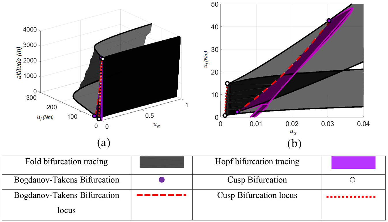
A bifurcation diagram with three-parameters, showing (a) the evolution of the bifurcations as altitude is raised from 0 to 4000 m and (b) a zoomed view in the load–throttle plane.
As before, as peak load torque varies with altitude, two-parameter continuations for altitude and peak load torque can be conducted to trace the fold loci and obtain the peak load torque for any altitude. Figure 19 provides insight into how altitude affects the peak load torque. It is observed that as altitude increases, the peak load available nonlinearly decreases.
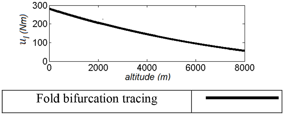
Two-parameter bifurcation diagrams, showing how peak load torque changes as altitude increases.
Parameters chosen in the design process may also be altered to determine how they affect the system’s dynamics. Figure 20 shows results for an increase (a) and decrease (b) in the size of the flywheel. The location of the fold bifurcation locus does not change qualitatively in either alteration; however, the throttle angle range in which the Hopf locus exists increases for a smaller flywheel and decreases for a larger flywheel. An even larger flywheel would cause the Bogdanov–Takens bifurcation to occur outside the physically meaningful range, which may explain why this sort of oscillatory behaviour is not typically observed in actual engines.
A three-parameter bifurcation diagram (a) and a zoomed two-parameter bifurcation diagram (b) showing the evolution of the bifurcations as engine inertia,
The bifurcation sensitivity analysis demonstrates how the locations of the fold and Hopf bifurcations are affected should additional parameters, such as lambda, ambient pressure, altitude and engine inertia, be deviated from their fixed value. Such deviations may occur during operation (altitude, pressure, lambda) or design (engine inertia). While no additional bifurcations were observed in the sensitivity study, the parameter values of the fold and Hopf bifurcations were observed to change. Changing the air flow parameters, such as changing altitude or ambient pressure, modified the parameter region in which the fold and Hopf bifurcations were observed. In comparison, changing the size of the flywheel moved the location of the Hopf bifurcation but not the fold bifurcations. These results demonstrate how a bifurcation analysis can be used to study parameter sensitivities: the analysis determines which type of modification, whether it be airflow or mechanical, will modify the parameter values that lead to certain types of dynamic behaviour (such as limit cycle oscillations).
Bifurcation analysis of a data-driven model
The bifurcation analysis so far has been used to demonstrate the range of dynamics found within a purely physics-based model; however, engine models often contain elements that are data-driven, that is, the dynamic model is built using data from a test cell. Here, a bifurcation analysis of this type of model is presented, in order to demonstrate the applicability of a bifurcation approach to a more industrial-oriented engine model. The data-driven model uses data that are discontinuous in nature, so to ensure smoothness, which is a pre-requisite for a bifurcation analysis, a cubic spline technique is used.
As before, a one-parameter continuation for different key torque values will show the qualitatively different behaviour in the system. It is important to distinguish between which areas of the state space are interpolated and which are extrapolated; therefore, this boundary is highlighted.
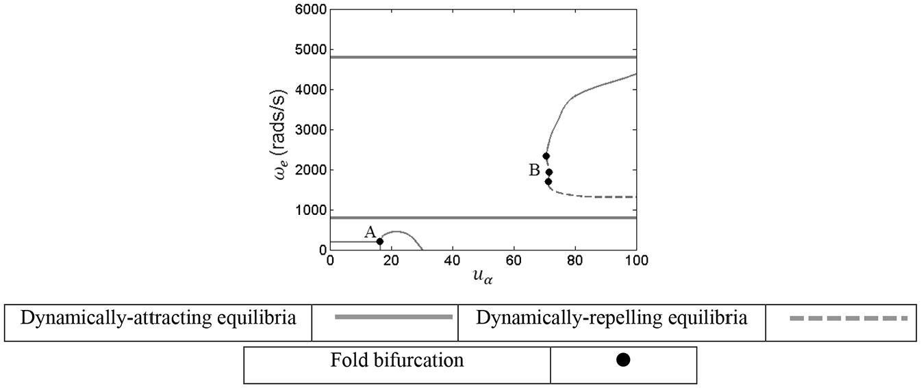
Figure 21 shows a one-parameter continuation for a torque input of 250Nm. Two separate branches are shown. The first branch is bound by two fold bifurcations: bifurcation A and another outside the physically meaningful throttle range. Horizontal lines indicate the extremities of the engine speed values at which data have been obtained. The first branch of equilibria, which is connected to bifurcation A, falls both inside and outside the region in which data exist. Those equilibria inside the region correspond to a steady-state output that could be achieved by the engine; those outside the region are produced from data extrapolation, so there are no data to support their existence. A second branch, connected to bifurcation B, is only present due to extrapolation. Although this appears outside the data range, this artefact is important as it shows the minimum engine speed required by the model to reach a realistic steady-state response. Engine speed initial conditions above branch B will be attracted to the steady-state output on branch A, while those below decay to zero.
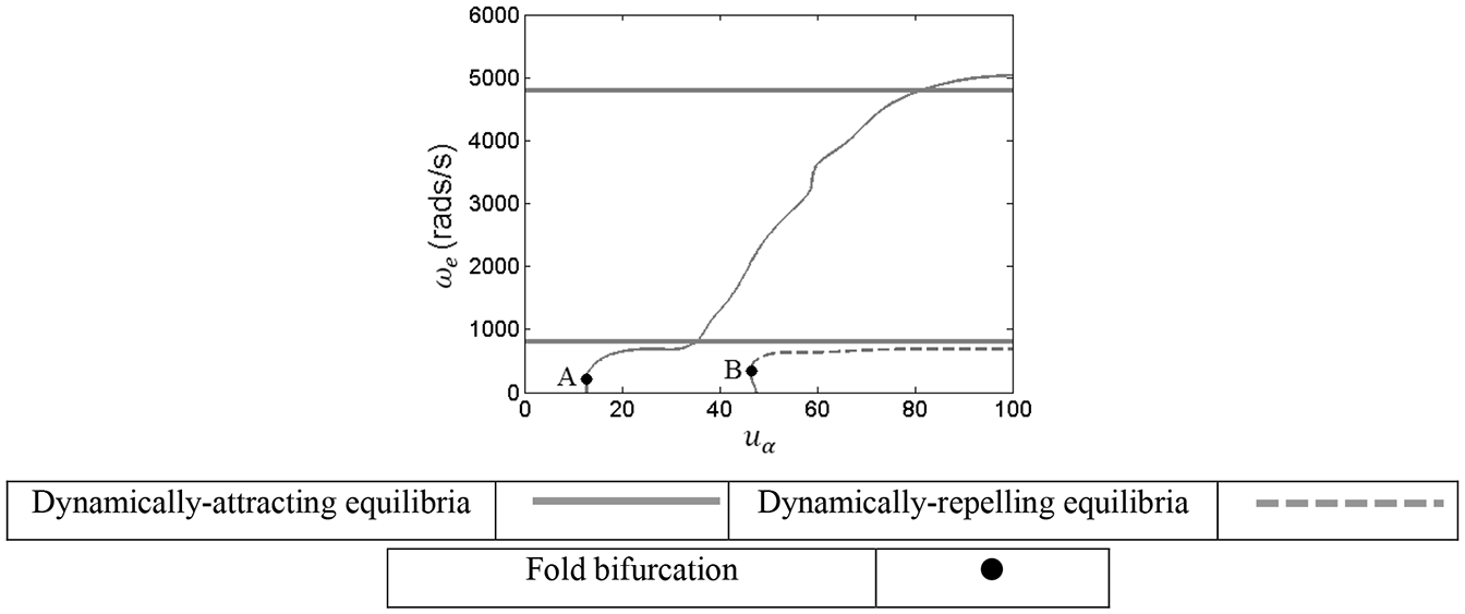
One-parameter continuation for
Figure 22 shows a one-parameter continuation for a torque input of 280Nm, where a qualitatively different response can be seen. Bifurcation A remains in a similar location; however, the associated branch is now entirely outside the data range and realistically the engine would never be able to run at any equilibria on this lower branch. The single branch that exists inside the data region is qualitatively the same as the one for the physics-based model in Figure 5(b) and therefore the same conclusions can be made. That is, the dynamically repelling equilibria highlight the minimum requirement on the initial condition for engine speed, and the fold bifurcation indicates the minimum throttle angle.
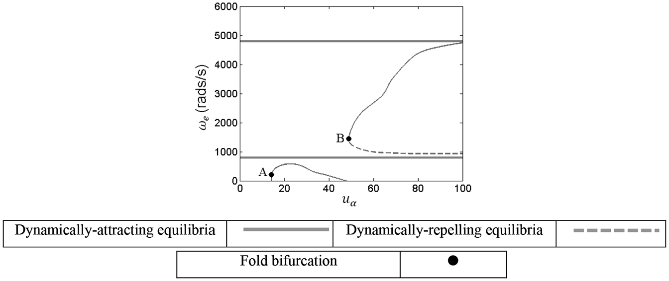
One-parameter continuation for
As before, these fold bifurcations can be traced through the entire state-parameter space. Figure 23 shows the parameter space (a) and state-parameter space (b). Three distinct branches are shown, A, B and C. Branches A and C are never within the data range; however, they bound dynamically attracting equilibria in the data range. Branch A can be seen in Figures 21 and 22 and bounds the lower branch. Branch C is out of bounds in Figure 21; however, this would represent the upper bound. Branch B traces the bifurcation present in Figures 21 and 22. In Figure 21, this point was out of bounds and was considered a dynamic artefact whereas in Figure 22, it was representative of a minimum throttle angle. The exact point in which the qualitative change happens is indicated by the cusp bifurcation.
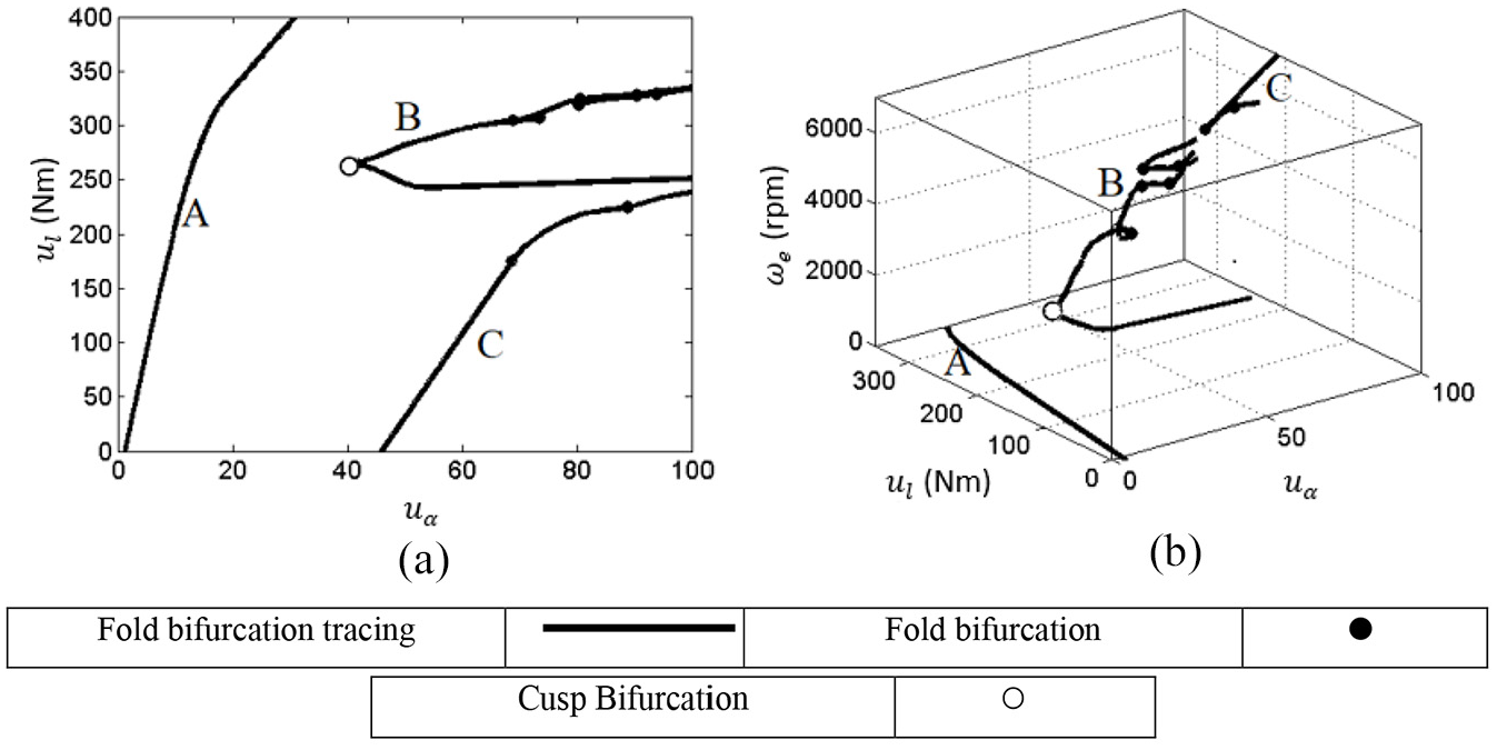
Parameter (a) and state-parameter space (b) for a two-parameter continuation for all possible
Many additional fold bifurcations exist on branch B. Figure 24 provides a one-parameter continuation in a dense area of fold bifurcation, which are described as ‘clusters’. There are no physical properties that would cause this behaviour, and as such, they are considered dynamic artefacts caused by interpolation. This clustering highlights that data gathered in this region are insufficient to determine the correct behaviour. Before any conclusions are made about this region, more operating points should be gathered in this region for a more complete and accurate analysis of this system.
One-parameter continuation for
Because there are only two parameters available to modify in this simple model, this completes the analysis; however, with more complicated models, a bifurcation sensitivity analysis could be conducted as demonstrated earlier.
Conclusion
This work offers a complementary approach to analyse the dynamics of a nonlinear engine model by conducting a bifurcation analysis. Two models were used: a physics model featuring three nonlinear first-order coupled differential equations and a smoothed data-driven model in Simulink. Both systems are mapped, and properties of the systems could be identified as bifurcation points in an efficient way using numerical continuation. Branches of dynamically repelling and dynamically attracting equilibria could be traced across the entire parameter range from a known steady-state response, allowing the user to predict the outcome of any time history simulation.
The equilibria traced in the system provides physical boundaries on the operation of the engine, with bifurcation points themselves indicating key system properties, such as the fold bifurcation being indicative of the minimum throttle angle and peak load torques, and Hopf bifurcations highlighting regions where oscillations occur in the system. A bifurcation sensitivity analysis provided further information about which changes in additional parameters may cause the system’s dynamics to qualitatively change. The regions in which the bifurcations exist in the state-parameter space change as alterations are made to the mechanical and/or air flow parameters.
There are many potential applications for the theory in automotive systems as the methods could be applied to any nonlinear powertrain model. Future areas to be considered include an emissions model to determine how emissions output is influenced by control parameters. In addition, knowledge of bifurcations and where qualitative changes in the engine’s dynamics response could aid engineers in the development and design of control strategies.
Footnotes
Declaration of conflicting interests
The author(s) declared no potential conflicts of interest with respect to the research, authorship, and/or publication of this article.
Funding
The author(s) disclosed receipt of the following financial support for the research, authorship, and/or publication of this article: This research is funded through the EPSRC Centre for Doctoral Training in Embedded Intelligence under grant reference EP/L014998/1, with industrial support from Jaguar Land Rover.