Sage Journals: Discover world-class research

Abstract

Transmissions require a good shift feeling and improved fuel efficiency. In state-of-the-art stepped automated transmissions, the number of gear stages increases, and the lock-up area is expanded to improve fuel efficiency. However, this makes it difficult to obtain a good shift feeling and it takes a large number of calibration man-hours. Therefore, to reduce the number of calibration man-hours and improve the shift feeling, we propose a slip control law between the engine and the clutch, which is composed of a proportional-integral-derivative (PID) controller and a disturbance observer. Moreover, PID gain is adjusted online by installing an automatic tuning method, which does not require a controlled object model. The effects of the proposed method are verified via an experiment using an actual vehicle. The experimental results show that the proposed method is effective for automatically adjusting PID gain and improving the shift feeling of the stepped automated transmission.

Keywords

Inertia phase gear shift self-tuning PID controller transmission clutch shift feeling

Introduction

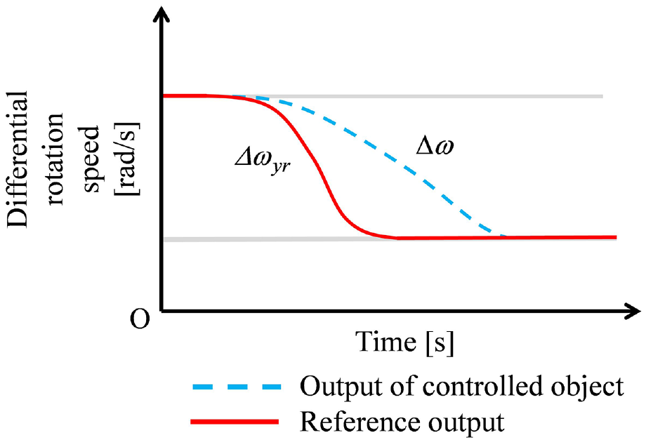
As components of automobiles, transmissions are required to have a good shift feeling and increasingly good fuel efficiency. To improve fuel efficiency, the number of gear stages of stepped automated transmissions with clutch-to-clutch shifting, such as automatic transmissions (ATs) and dual clutch transmissions (DCTs), has been increased, and in vehicles with torque converters, the area of the lock-up, which directly transfers engine power to the transmission without oil, has been expanded. As the shifting frequency in automated transmissions increases to become more multistage, a slight shift shock causes discomfort to the driver and leads to deterioration of the durability of the product. In conventional shift control, the shift shock is absorbed by the fluid of the torque converter without lock-up, but in recent years, slip control law of the torque converter using the lock-up clutch has been studied to achieve both improvements in fuel efficiency and reduction in shift shock.^1–5 To realize slip control of the torque converter by implementing a lock-up mechanism, in addition to the multiplication of the lock-up clutch, changing the piston chamber and damper, and adding a proportional valve, a new configuration of the control system is required, which increases cost. Moreover, some vehicles are not equipped with a torque converter. Therefore, it is desirable to reduce the transmission shock by clutch control of the transmission without relying on slip control of the torque converter by the lock-up clutch. Figure 1 shows a shift process during an upshift. If the clutch is contacted when the angular acceleration of the engine is high, a shift shock occurs, as shown in Figure 1 (broken line). To reduce transmission shock, the engine angular acceleration must be reduced during the synchronization between the engine and the clutch output shaft rotational speed (i.e. when the differential rotation speed between the engine and clutch output shaft becomes zero). However, to reduce the contact shock, if the shift time is simply lengthened, as shown in Figure 1 (dotted line), slow feeling shift occurs, which leads to discomfort to the driver and a decrease in clutch life. These problems arise when the engine speed or the differential speed between the engine speed and the clutch output shaft speed cannot achieve the target value. Hence, by realizing control system design that follows the target value, it is possible to realize a shift without the slow sense or shock. In addition to the target value shown in Figure 1, when the clutch capacity is sufficient, slip control⁶ is also performed in which the vehicle travels while generating the differential rotation speed to avoid a shift shock.

Figure 1.

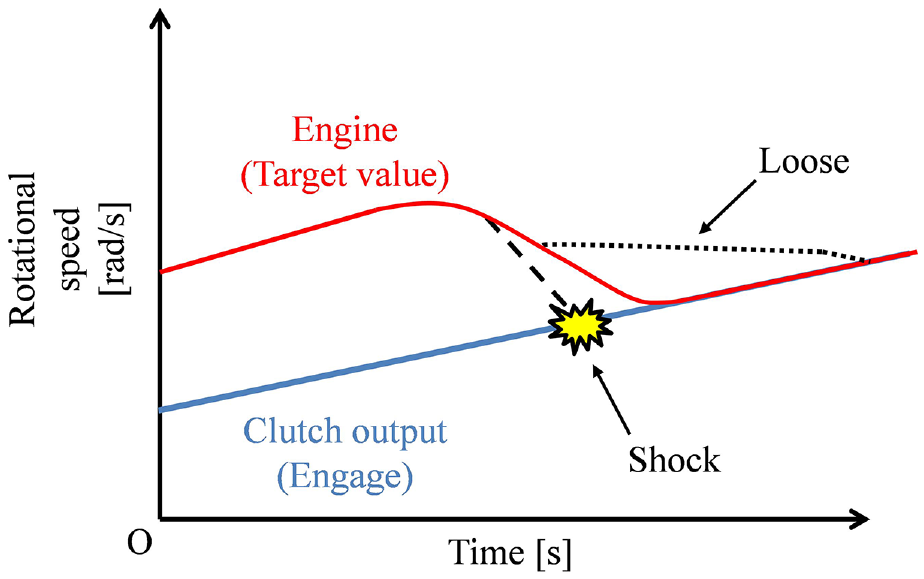
Rotational speed over time showing the cause of shift shock.

Control law during the inertia phase of an automated transmission has been studied in various ways by using model-based control.^7–13 For example, it is possible to study differential rotation speed control by using robust control such as H_∞ control. Although H_∞ control can ensure stability by considering the modeling error in advance, it is usually necessary to estimate the large modeling error when a multi-domain complex system like an AT, which includes hydraulic, electric, and mechanical domains, is targeted. Thus, the designed controller becomes conservative. Furthermore, the order of the controller must be lowered so that it can be mounted on the mass production controller. Know-how is required to achieve good performance. It should be noted that a reduction in number of development man-hours is required, but it takes man-hours to obtain an accurate mathematical model. Also, it may be difficult to obtain highly accurate models in real systems in the industry. In commercial systems, most control systems are feed-forward control and proportional–integral–derivative (PID) control, which are easy to understand. In particular, PID control is used in more than 90% of industrial control loops.¹⁴ However, PID control requires calibration to adjust the control parameters. In recent years, the rapid increase of electronic control has caused a problematic increase in the number of calibration man-hours.⁵ Considering this background, studies have been carried out on model-free control and reducing the number of calibration man-hours.^15–22

This paper proposes a differential rotation speed control law (in other words, a slip control law) that realizes reduced shock during the inertia phase by slip control of a transmission for a stepped automated transmission with clutch-to-clutch shifting. Automatic PID gain adjustment uses fictitious reference iterative tuning (FRIT) and recursive least square (RLS)-based controller adjustment techniques^23,24 that do not require a controlled object model. There have been no prior studies on applying FRIT to automotive systems, particularly automated transmissions and their experimental verification, because FRIT is a relatively new technique. Most FRIT applications involve simple experimental equipment and plants in which PID controllers are used in large quantities. The conventional slip control law for an automated transmission does not cooperatively control the engine and automated transmission. Such conventional control systems have not been designed to be suitable for applying FRIT to adjust the feedback linear controller parameters. Particularly, because the clutch torque is operated according to the conventional slip control law, a trade-off with drivability occurs, and complicated modeling of the clutch is required. In light of these factors, linear feedback control cannot be constructed, and it is difficult to automatically adjust all the parameters. Furthermore, experimental verification using actual industrial machines is also a hurdle and is likely the reason why there has been no automotive application. This paper proposes a linear feedback control law in which the engine torque is used as the manipulated variable by performing cooperative control of the engine and the automated transmission; this allows the slip control law to be implemented in a linear controller, which facilitates the application of FRIT. A reduction in the number of calibration man-hours and a good shift feeling are expected by automatically adjusting the controller parameters of the proposed control law.

The structure of this paper is described as follows. The “Introduction” describes the necessity of the stepped transmission, its problems, and the importance of the control method without using a model. The “System overview” section explains the controlled object by using a simple model of the automated transmission with clutch-to-clutch shifting. In “Slip speed control” section, a closed-loop system is constructed by using a PID controller and a disturbance observer for slip control. Furthermore, the FRIT–RLStechnique^23,24 for automatically adjusting the PID gain is briefly described. The “Experimental verification” section experimentally verifies the effect of the control law constructed in the “Slip speed control” section by using an actual vehicle. The results show that clutch control of the transmission according to the proposed method can realize slip control and shifting without extension or shock. The “Conclusion” section discusses the conclusions of this paper.

System overview

Controlled object

Figure 2 shows a simplified model of a controlled object. The controlled object includes an engine, a plurality of clutches, and gears. T_e, T_clt, T_o, ω_e, ω_clt, and ω_o are the engine torque, the clutch torque, the output shaft torque of the automated transmission, the engine rotation speed, the clutch output rotation speed, and the output shaft rotation speed of the automated transmission, respectively. Subscripts A and B represent clutches A and B, respectively. Next, the shift process during an upshift is shown in Figure 3. There is a torque phase in which the clutch is replaced during an upshift, and there is an inertia phase during which a change in the engine speed takes place.²⁵ In the inertia phase, it is important to reduce the slow feeling and shock that occur when the engine and clutch output shaft rotation speed are synchronized (i.e. when the differential rotation speed between the engine rotation speed and the clutch output shaft rotation speed becomes zero). As shown by the broken line in Figure 1, a shock occurs when the engine rotation angular acceleration at the differential rotation speed 0 is large. Note that the torque converter is not shown in Figure 2 because it is in the lock-up state during the shift.

Figure 2.

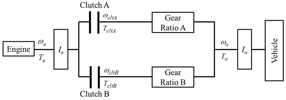
Simplified vehicle system with a stepped transmission.

Figure 3.

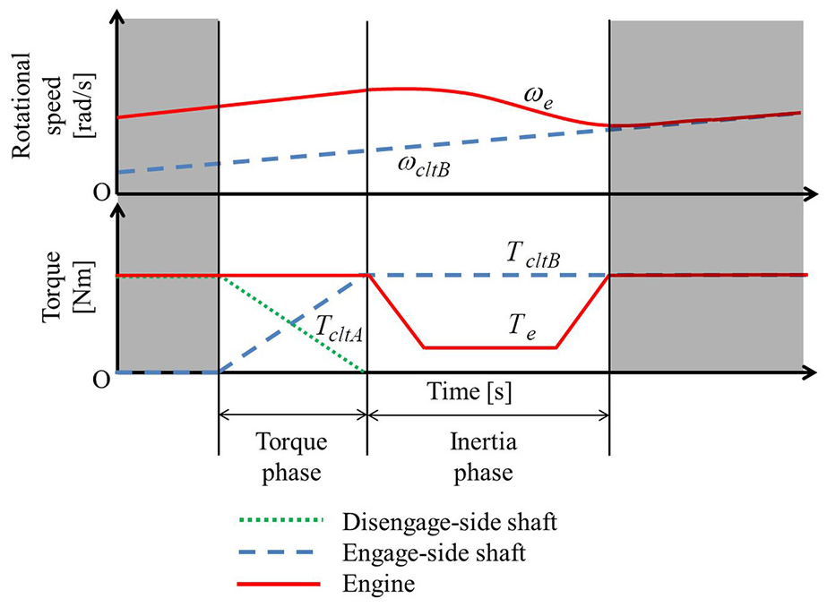
Shift process.

Motion model during the inertia phase

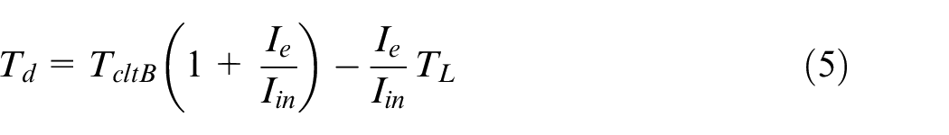
During the inertia phase, the clutches A and B are in a slip state. The equations of motion of the engine shaft and the clutch output shaft are expressed by equation (1). The shift is realized by generating engine and clutch torque. Note that the actual drivetrain model is more complicated, but we describe a very simplified model because the online automatic PID tuning method subsequently described in “Slip speed control” section does not require a controlled object model

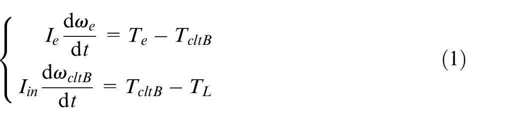
{\begin{matrix} I_{e} \frac{d ω_{e}}{d t} = T_{e} - T_{cltB} \\ I_{in} \frac{d ω_{cltB}}{d t} = T_{cltB} - T_{L} \end{matrix}

(1)

where I_in is the equivalent moment of inertia of the vehicle (the sum of the vehicle-side rotation inertia converted on the clutch), T_L is the driving resistance torque, and F_L is the driving resistance. T_L and F_L are expressed by equation (2)

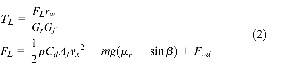
\begin{matrix} T_{L} = \frac{F_{L} r_{w}}{G_{r} G_{f}} \\ F_{L} = \frac{1}{2} ρ C_{d} A_{f} {v_{x}}^{2} + mg (μ_{r} + \sin β) + F_{wd} \end{matrix}

(2)

where G_r, G_f, r_w, ρ, C_d, A_f, m, g, μ_r, β, and F_wd are gear ratio, final stage gear ratio, tire dynamic radius, air density, resistance coefficient, projected area on the front surface, vehicle weight, gravitational acceleration, rolling resistance coefficient, road gradient, and disturbance, respectively. T_cltB is the clutch torque acting on the engaging-side shaft and is expressed by equation (3)

\begin{matrix} T_{cltB} = μ RN (A P_{cB} - F_{rtrn}) \\ P_{cB} = f (i_{vlvB}) \end{matrix}

(3)

where μ, R, N, A, P_cB, F_rtrn, and i_vlvB are clutch frictional coefficients, clutch effective radius, the number of clutch contacting surfaces, piston pressure receiving area, hydraulic pressure in the clutch piston chamber, clutch spring reaction force, and the current of the pressure proportional valve, respectively; note that f represents a function. The clutch torque is correlated with the pressure in the clutch piston chamber. The pressure in the piston chamber is generated by applying current to the pressure proportional valve, that is, clutch torque is generated by applying current to the pressure proportional valve. The relationship between the current and pressure is nonlinear, and the characteristic differs depending on each pressure proportional valve.

Relationship between the controllers and a controlled object

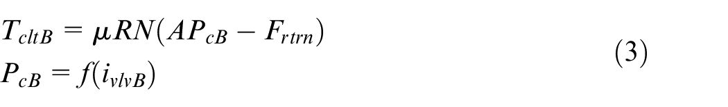
The vehicle system comprises a plurality of controllers. The respective controllers exchange various signals by controller area network (CAN) communication. The relationship between the transmission control module (TCM), engine control module (ECM), transmission, and engine can be described as follows. Figure 4 shows the main component of the shift control during the inertia phase. Q_fuel is the fuel injection quantity, ^ represents the estimated value, and the subscript cmd represents an instruction value. The content described in “Slip speed control” section is implemented in the TCM. The engine torque instruction value is sent by the TCM to the ECM by CAN communication. The engine torque is generated by informing the engine of the fuel injection quantity calculated by the engine torque controller in the ECM. Furthermore, the engine torque estimated by the torque estimator in the ECM is transmitted to the TCM. The engine speed obtained by the sensor and the electronic circuit in the ECM is transmitted to the TCM by CAN communication. The engine torque commanded by the TCM is sent to the ECM by CAN communication. This engine torque is obtained by the proposed slip speed controller in the TCM described later. The clutch output shaft speed is generated by informing the transmission of the clutch valve current calculated in the TCM. The clutch output shaft speed is obtained by the sensor and the electronic circuit in the TCM. The clutch valve current is calculated to meet the driver requested torque, which is calculated from the driver’s accelerator pedal position and engine speed.

Figure 4.

Vehicle system controllers and controlled objects.

Slip speed control

After introducing an outline of the shift control during the inertia phase, we explain the feedback control system using a PID controller that is constructed to realize the differential rotation speed control of the clutch and engine. In addition, we discuss a disturbance observer and self-tuning PID control that are introduced to cope with changes in the clutch characteristics and reduce the number of calibration man-hours.

Outline of shift control during inertia phase

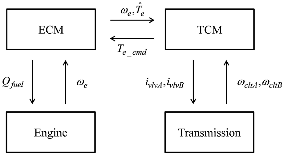
The outline of the basic control of the engine and clutch in the inertia phase is described here. Figure 5 shows the process of generating the clutch and engine torque; α is the driver’s accelerator pedal position, Δω is the amount of slip rotation between the engine rotation speed and clutch output engage-side shaft rotation speed. First, the driver requested torque is calculated from driver’s accelerator pedal position and engine speed. The driver requested torque is the target clutch torque on the engine shaft. A current to be applied to the valve is calculated from the driver requested torque by using the equation correlating the clutch torque and the pressure (Equation 3). The clutch torque is then generated by applying the calculated valve current. This enables the driver to generate the intended driving force. Because the clutch torque generates the driver demand torque, the engine torque is used as a manipulated variable to control the engine speed or the differential speed; that is, the engine speed control or the differential rotation speed control are performed using the engine torque as a control input to the engine.

Figure 5.

Overview of shift control during inertia phase.

In the previously proposed differential rotation control law,^10–12 the driver requested torque cannot be generated by the clutch torque because the valve current that manipulates the clutch torque is used in the manipulated variable for slip control. Thus, the output shaft torque of the transmission fluctuates, and a favorable transmission feeling cannot be obtained. To reduce the torque fluctuation, the engine torque is given as a feed-forward term.^11,12 However, the logic is not explained, and if the feed-forward term is not appropriate, the driver's intended acceleration will not be achieved. In comparison, in the method proposed in this paper, the driver-required torque is generated by the clutch torque, and the differential rotation speed control is performed by using the engine torque as the manipulated variable; the shift leading to the driver’s intended acceleration can be realized during the inertia phase.

Slip speed control law between engine and clutch

A feedback control law for realizing differential rotation speed control is derived. When equation (1) is rearranged, the equation of motion for the differential rotation speed is as follows

I_{e} \frac{d Δ ω}{d t} = T_{e} - T_{d}

(4)

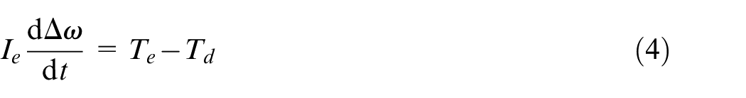
with

T_{d} = T_{cltB} (1 + \frac{I_{e}}{I_{in}}) - \frac{I_{e}}{I_{in}} T_{L}

(5)

Δ ω = ω_{e} - ω_{cltB}

(6)

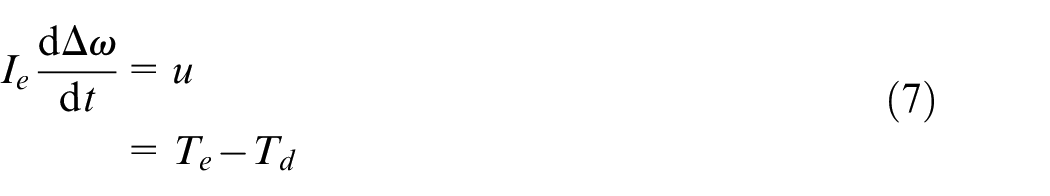
T_d can be regarded as a disturbance torque. Therefore, let the right side of equation (4) be the control input of the PID controller, according to equation (7)

\begin{matrix} I_{e} \frac{d Δ ω}{d t} = u \\ = T_{e} - T_{d} \end{matrix}

(7)

The PID controller C(s, θ) is given by equation (8)

C (s, θ) = θ^{T} ϕ (s)

(8)

Here

\begin{matrix} θ = {[θ_{p} θ_{i} θ_{d}]}^{T} \\ θ (s) = {[\begin{matrix} 1 & \frac{1}{s} & \frac{s}{τ^{p i d} s + 1} \end{matrix}]}^{T} \end{matrix}

(9)

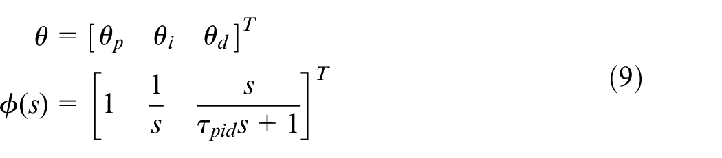
where θ, θ_p, θ_i, θ_d, and τ_pid are control parameter vectors, proportional gains, integral gains, differential gains, and time constants of an approximate differentiator, respectively, and the symbol s represents a Laplace operator. The information sent to the engine is the required value of engine torque and is expressed by equation (10)

T_{e_c m d} = u + T_{d}

(10)

Therefore, it is necessary to know the disturbance torque T_d. Here, the disturbance torque is estimated using the disturbance observer,^26–28 as shown in the following equation

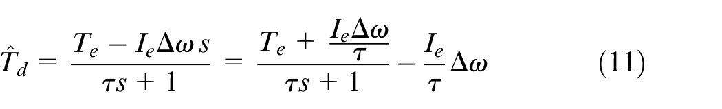
{\hat{T}}_{d} = \frac{T_{e} - I_{e} Δ ω s}{τ s + 1} = \frac{T_{e} + \frac{I_{e} Δ ω}{τ}}{τ s + 1} - \frac{I_{e}}{τ} Δ ω

(11)

where τ is the low-pass filter time constant. First, we describe the methods to determine the parameter by the general theory. The time constant should be small based on the estimated velocity. However, possibly, the correct estimation cannot be performed owing to the influence of observation noise. In other words, there is a trade-off to determine the time constant. Next, we explain the method to determine the parameter for the proposed slip controller. When the differentiation is performed with a small time constant, the estimated disturbance torque becomes oscillatory for the observation noise. Thus, the engine command torque also becomes oscillatory; this leads to driver discomfort. However, the estimation must follow changes in the disturbance torque including the driver requested torque and the load torque. In practice, the time constant should be chosen so that the estimated disturbance torque does not oscillate.

We can see that by using the disturbance observer in equation (11), calibration parameters significantly reduce and the disturbance torque can be estimated more simply. If the disturbance observer is not adopted, disturbance torque is obtained from equation (5), which includes engine inertia, vehicle-side rotational inertia, clutch torque, and driving resistance. Therefore, there is substantial calibration cost requirement for the system identification to obtain parameters in equation (5). Moreover, methods to estimate the clutch torque and the driving resistance must be established. Therefore, we believe that the disturbance observer is effective to simplify the estimation of the disturbance torque.

As described in equations (8) and (11), the three parameters required for the design of the slip control law are the PID gain θ, the low-pass filter time constant τ of the disturbance observer, and the engine inertia I_e. However, the PID gain is automatically adjusted (as described later), and the time constant used in the disturbance observer is easily determined. The engine inertia is readily obtained by checking the design information or system identification.

The control structure is shown in Figure 6. The PID gain is optimized by the automatic adjustment mechanism described in ``Automatic PID gain adjustment mechanism'' section.

Figure 6.

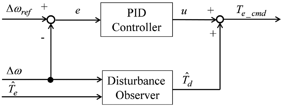
Block diagram of the slip controller.

Automatic PID gain adjustment mechanism

An automatic PID gain adjustment mechanism is introduced to cope with characteristic variations caused by aging or temperature changes as well as to reduce the number of calibration man-hours. FRIT has been proposed as a method for automatically tuning control parameters off-line without a controlled object model using only a set of input/output data. We believe that using this method can reduce the number of calibration man-hours. Furthermore, an online FRIT combining FRIT and RLS has been proposed.^23,24

Standard FRIT

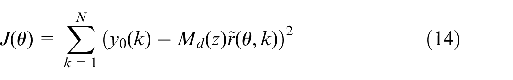
This section describes the standard FRIT. In Figure 7, a general feedback control system and a reference model are shown. M_d is a reference model representing a target response transfer function (target complementary sensitivity function) from the target value r to the control variable y, and z represents a shift operator. The reference model is determined by a designer, and its modeling does not require the mathematical model of the controlled object. We explain a design method of the reference model later. Standard FRIT determines the controller parameters to minimize the following objective functions

J_{0} (θ) = \sum_{k = 1}^{N} {(y (k, θ) - M_{d} (z) r (k))}^{2}

(12)

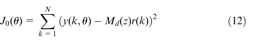
Hence, the controlled object brings the response of the control target closer to the reference model response.

Figure 7.

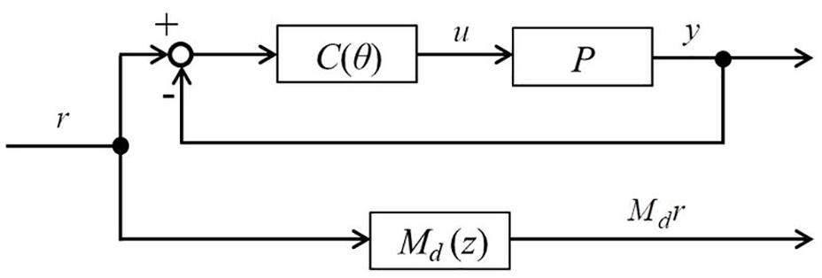
Closed system and reference model with tunable parameters.

Considering FRIT procedures, first, closed-loop experiments are performed using initial controller parameters that stabilize the system, and time-series data u₀ and y₀ of the input and output are acquired. Next, the acquired initial input/output time-series data and the controller are used to calculate the fictitious reference signal²⁹ shown in equation (13)

\tilde{r} (θ, k) = C^{- 1} (θ) u_{0} (k) + y_{0} (k)

(13)

Based on the fictitious reference signal, the controller parameters for which the following objective function is minimized are determined by an optimization method. The standard FRIT uses off-line calculations

J (θ) = \sum_{k = 1}^{N} {(y_{0} (k) - M_{d} (z) \tilde{r} (θ, k))}^{2}

(14)

We consider the case where the aforementioned content is replaced with slip control, as shown in Figure 8. Thus, we obtain equation (15)

J (θ) = \sum_{k = 1}^{N} {(Δ ω_{yr} (k) - Δ ω (k))}^{2}

(15)

In equation (15)

Δ ω_{yr} (k) = M_{d} (z) Δ ω_{ref} (k)

(16)

Figure 8.

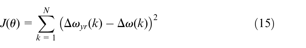
Slip control using FRIT.

Online FRIT

Because standard FRIT has a nonlinear objective function, the computational cost of performing online calculations is high. In online FRIT, the computational cost is reduced by transforming the optimization problem to be solved into a least squares problem and solving the optimization problem by the RLS method. To make the objective function a least squares problem, equation (12) is modified.

Considering the ideal case where the objective function is zero, equation (12) is obtained

y_{0} (k) - M_{d} (z) \tilde{r} (θ, k) = 0

(17)

Substituting this equation into equation (13) yields

C (θ) y_{0} (k) - M_{d} (z) u_{0} (k) - C (θ) M_{d} (z) y_{0} (k) = 0

(18)

Focusing on equation (18), an objective function such as equation (19) is minimized

\hat{J} (θ) = \sum_{k = 1}^{N} {\hat{e}}^{2} (k)

(19)

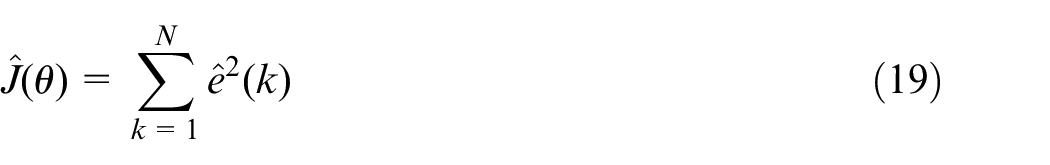
with

\hat{e} (k) = C (θ) (1 - M_{d} (z)) y_{0} (k) - M_{d} (z) u_{0} (k)

(20)

We replace the initial input/output data u₀ and y₀ with the input/output u and y (sequentially measured) and organize equation (20) as follows

C (θ) = θ^{T} ϕ (z)

(21)

ξ (k) = ϕ (z) (1 - M_{d} (z)) y (k)

(22)

d = M_{d} (z) u (k)

(23)

where $ϕ (z)$ is obtained by discretizing $ϕ (s)$ . Then, equation (20) is as follows

\hat{e} (k) = θ^{T} ξ (k) - d (k)

(24)

We can see that the error $\hat{e}$ can be expressed in a linear form with respect to θ. The RLS with the forgetting factor is implemented to minimize the linearized objective function for online calculation. The RLS algorithm with forgetting factor is found in equations (25)–(27)³⁰

\hat{θ} (k) = \hat{θ} (k - 1) + K (k) (d (k) - ξ^{T} (k) \hat{θ} (k - 1))

(25)

K (k) = \frac{P (k - 1) ξ (k)}{λ + ξ^{T} (k) P (k - 1) ξ (k)}

(26)

P (k) = \frac{1}{λ} {P (k - 1) - \frac{P (k - 1) ξ (k) ξ^{T} (k) P (k - 1)}{λ + ξ^{T} (k) P (k - 1) ξ (k)}}

(27)

where P is the covariance matrix, and λ is the forgetting factor. In the online FRIT, to prevent instability of the system due to a rapid parameter change of the controller, it has been proposed that an implemented controller parameter is updated by equation (28), which is also used in this paper

θ (k) = (1 - γ) θ (k - 1) + γ \hat{θ} (k - 1)

(28)

where γ is a small positive number.

Design of the reference model for slip control

We describe the design of the reference model for slip control. Note that the controlled object model is not required for designing the reference model, as described in “Standard FRIT” section. A designer determines an ideal response. For the slip control, we recommend a reference response without overshoot because the differential rotation speed between the engine and clutch output shaft should be zero to avoid transmission shock at the synchronization point. The n-order transfer function, shown in equation (29), is known as the reference model that does not induce overshoot because all poles exhibit a negative real part³¹

M_{d} (s) = \frac{p^{n}}{{(s + p)}^{n}}

(29)

where p is the parameter for determining the responsiveness. The design parameter n is chosen considering the computational cost; in a previous study,¹¹ third order was used. The parameter p is chosen considering the clutch durability and engine inertia, the maximum torque, and so on. Moreover, we consider the case that the controlled object has dead time. It’s impossible for the controlled object response to track a reference response whose dead time is shorter than that of the controlled object. Because this limitation of dead time is related to the inherent characteristics that cannot be improved by controllers, the reference model, including the dead time, is used as³²

M_{d} (s) = \frac{p^{n}}{{(s + p)}^{n}} e^{- sL}

(30)

where L is the estimated dead time of the controlled object. In FRIT–RLS, the error $\hat{e}$ must be a linear form with respect to the optimizing parameters to use the RLS algorithm in equation (24). However, when the optimizing parameters include dead time, the error $\hat{e}$ is not linear with respect to the optimizing parameters, including the dead time. Thus, we determine the dead time, included in equation (30), in advance instead of including the dead time in the optimizing parameters. A designer needs to estimate the dead time to design the reference model. Hence, the transfer function form and the parameters n and p are determined without using a controlled object model. The parameter L should be determined based on information from the controlled object.

Experimental verification

Outline of the experiment

An overview of the system is shown in Figure 9. The test vehicle is a medium-sized truck (total vehicle weight is 8 tons), and the diesel engine used is a 4HK1-TCS (Type: 4 cylinders OHC direct injection diesel, displacement: 5193 cc, compression ratio: 16.5, maximum power: 154 kW/2400 r/min, maximum torque: 706 N m/1400–1600 r/min). The transmission (T/M) is a stepped automated transmission with clutch change (torque converter is installed, wet multi-plate clutches are used). The ECM uses conventional controllers produced in large volumes, and the TCM uses dSPACE’s Rapid Prototyping System (MABX^® and RapidPro^®). The created program is implemented in MABXII^®, and the programing language is MATLAB/Simulink. The sampling period of the TCM and ECM is 8 ms. Signals of various controllers are communicated by CAN. The transmission of the engine torque from the TCM to ECM requires approximately 30 ms, and the engine speed is sent from the TCM to the ECM in 10 ms. Then, after the lock-up clutch of the torque converter is engaged, the upshift is performed. The time-series data sent from MABXII^® to the notebook PCs are measured for the various signals.

Figure 9.

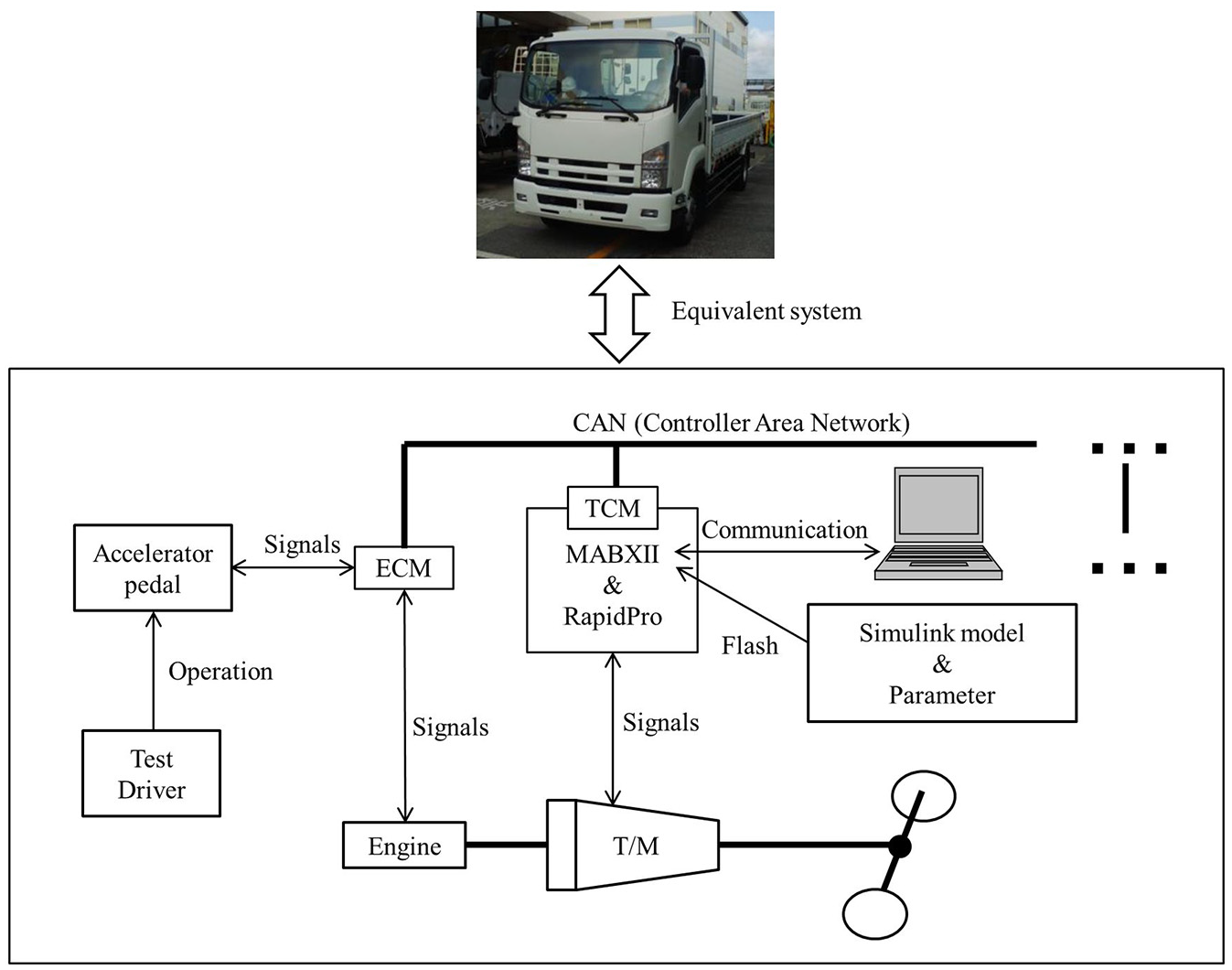
Overview of the experimental system.

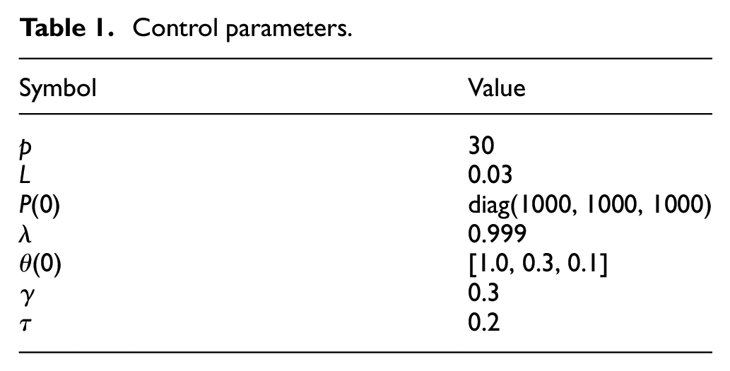
The parameters for the reference model, RLS algorithm, and disturbance observer are shown in Table 1. The reference model uses the transfer function in equation (30). We adopt the third order as performed in a previous study.¹¹ Regarding the dead time in equation (30), see Figure 5; the engine torque is generated by providing the ECM with the value calculated by the TCM, calculating the fuel injection quantity for generating the requested torque in the ECM, and applying the calculated fuel injection value to the engine, that is, the requested engine torque and the actual torque are not completely the same. The actual engine torque generation mechanism is very complicated, but in this paper, the relationship between the requested engine torque value and the actual value is approximated by the dead time L in equation (31). Thus, a dead time occurs from the time when the engine torque value is requested to the time when the actual engine torque is generated. This approximation is reasonable from the experimental results described in “Experimental results and discussion” section

T_{e} = T_{e_c m d} e^{- Ls}

(31)

Table 1.

Control parameters.

Symbol	Value
p	30
L	0.03
P(0)	diag(1000, 1000, 1000)
λ	0.999
θ(0)	[1.0, 0.3, 0.1]
γ	0.3
τ	0.2

Experimental results and discussion

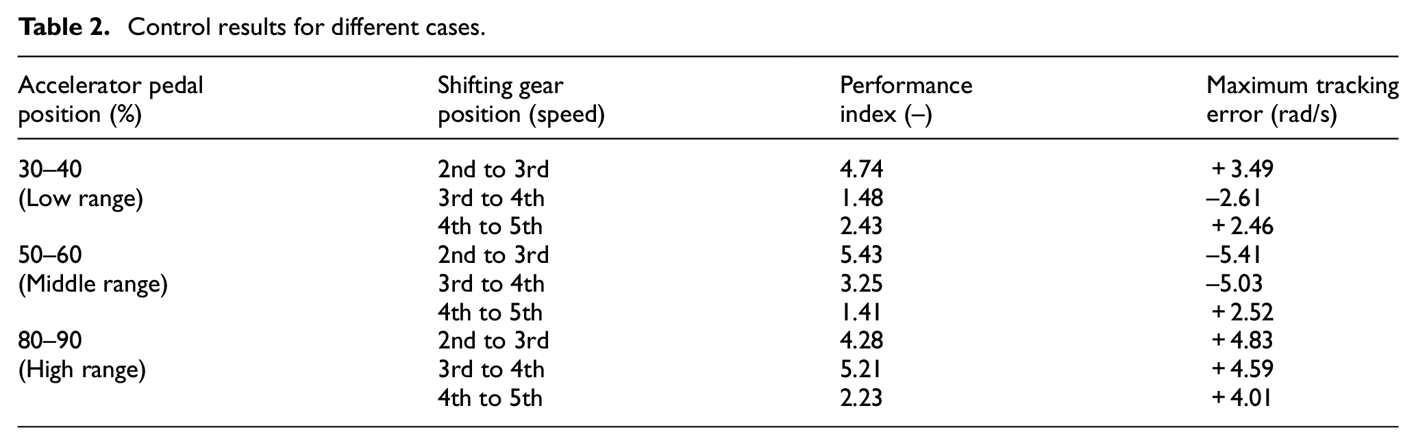
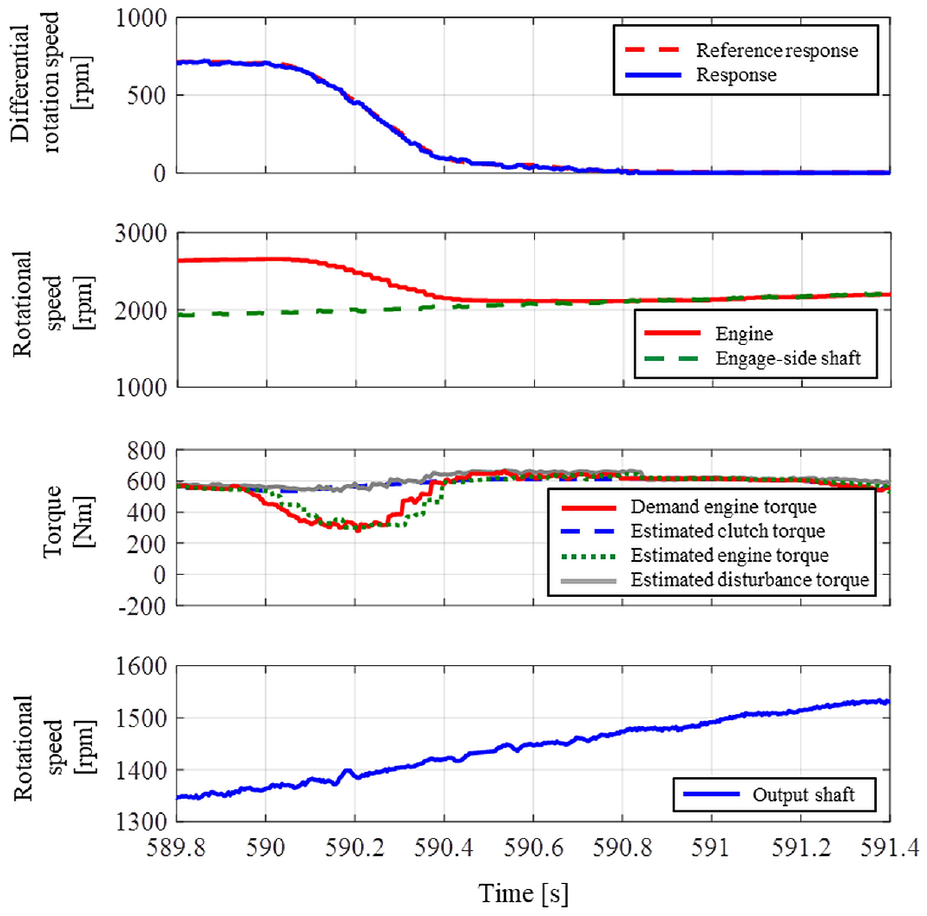
Figure 10 shows time-series data obtained when the shift-up from the second to the third speed and the shift-up from the third to the fourth speed are performed under the condition that the target differential rotation speed is set to 200 r/min and the PID gain is set to an appropriate initial value. Here, the second speed means the gear position in a commercial vehicle launch. The horizontal axis represents time, and the temporal developments of the differential rotation speed, indicated torque, proportional gain, integral gain, and differential gain are shown in each plot. From the figure, we can see that the PID gain is automatically tuned and follows the target value in one shift. In Figure 11, time-series data are plotted for the clutch being smoothly engaged during the inertia phase with the adjusted PID gain. The change in the differential rotation speed, rotational speed, indicated torque, and the transmission output shaft speed over time are shown in the plots. We see that the engine speed can be smoothly connected to the engage-side shaft, and the shift is completed without inducing a shock or a slow feeling. Moreover, based on the rotation speed of the transmission output shaft, it is confirmed that no extreme fluctuation is present, and the fluctuation level is almost the same before and after synchronization. Therefore, we consider the shift shock to be extremely small. Table 2 shows the performance index that normalizes equation (15) by the inertia phase time and maximum tracking error for the differential accelerator pedal position and shifting gear position. The conditions for accelerator pedal position are the low, middle, and high range, and for the gear shift speed, the conditions are from second to third, from third to fourth, and from fourth to fifth speed. Based on the results of the performance index, the proposed method realizes the same level of performance in every case with various accelerator pedal and shift positions. Also, the maximum tracking error in every case is 5.41 rad/s (51.7 r/min). Therefore, we consider that the proposed method realizes target slip control with approximately 50 r/min. Figure 12 shows the experimental result for a target differential rotation speed of 50 r/min. The horizontal axis represents time, and the temporal developments of the differential rotation speed, rotation speed, and torque are shown in each plot. The controlled object response can track the target response. Therefore, the results confirm that the constructed differential rotation speed control law with PID automatic adjustment is capable of obtaining a good upshift feeling without prior calibration.

Table 2.

Control results for different cases.

Accelerator pedalposition (%)	Shifting gearposition (speed)	Performanceindex (–)	Maximum trackingerror (rad/s)
30–40	2nd to 3rd	4.74	+3.49
(Low range)	3rd to 4th	1.48	–2.61
	4th to 5th	2.43	+2.46
50–60	2nd to 3rd	5.43	–5.41
(Middle range)	3rd to 4th	3.25	–5.03
	4th to 5th	1.41	+2.52
80–90	2nd to 3rd	4.28	+4.83
(High range)	3rd to 4th	5.21	+4.59
	4th to 5th	2.23	+4.01

Figure 10.

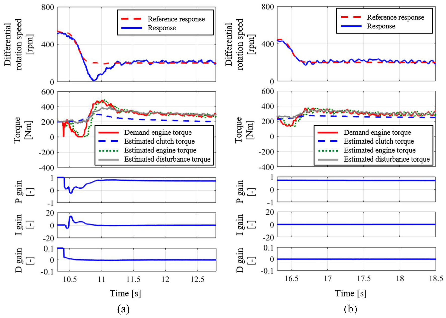
Upshift slip control: (a) Upshift (first time) and (b) upshift (second time).

Figure 11.

Ideal upshift control.

Figure 12.

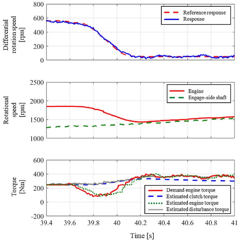
Shift-up control for a target differential rotation speed of 50 r/min.

We consider the reasons for the automatically adjusted differential and integral gains to approach almost zero. First, the integration approaches almost zero because of the effects of the disturbance observer and the dead time. Although the integral term of the PID controller is used to cancel the steady state deviation, the proposed method includes a disturbance observer; the removal of the steady state deviation is considered to be compensated by the disturbance observer rather than the integral term of the PID controller, that is, all torques other than the nominal inertial acceleration/deceleration torque $(I_{e} (d Δ ω / d t))$ are regarded as equivalent disturbance, and the constructed disturbance observer simultaneously compensates them all.²⁶ Moreover, the control system, including the controlled object and the disturbance observer designed herein, has an integral factor, type 1 system, during the steady state (see Appendix 1). Thus, the steady state deviation theoretically becomes zero. As described above, because the disturbance observer cancels the steady state deviation, the integration gain becomes very small. Regarding the influence of the dead time, if the integration term becomes large by integrating the error during the dead time, the control input becomes excessively large, and the control system becomes unstable in some cases. Because the reference model used in this experiment is a system with a relatively slow response, undershoot occurs with respect to the target response when the integral term excessively increases the control input. In addition, for systems in which phase lag occurs because of dead time, it may be undesirable to further delay the phase from a stability standpoint because the integral term is a phase lag component. We suggest that the integral term becomes almost zero due to the effect of the disturbance observer and the influence of the dead time. Considering why the differential gain approaches zero, it is important to remember that the differential term of the PID control is effective in improving the transient characteristic, that is, although the differential term is used to improve the response in the high frequency region, the target response in this experiment exhibits a relatively gradual characteristic with respect to the target value, whereby the gain in the high frequency region does not need to be increased. Therefore, the differential gain becomes almost zero.

Conclusion

A new slip control law is proposed for shifting during the inertia phase of a stepped automated transmission with clutch-to-clutch shifting. The proposed control law consists of a PID controller and a disturbance observer. The PID gain is automatically adjusted by installing an FRIT–RLS method. The proposed method was experimentally verified by an actual vehicle test. The results confirmed that the PID gain can be adjusted by one shift, and the amount of slip can achieve the target response. Also, the engine and clutch rotation speed on both sides are synchronized smoothly to realize the desired shift. Based on these results, it can be concluded that the proposed method is effective in reducing the number of calibration man-hours and improving the shift feeling in a stepped automated transmission.

Footnotes

Appendix 1

We describe the disturbance observer and the reason a system, including controlled object and disturbance observer, is a type 1 system during the steady state. Here, the type 1 system includes an integral factor.³³ The block diagram of the disturbance observer used in the slip control is shown in Figure 13. It’s assumed that T_e, T_{e_cmd}, and ${\hat{T}}_{e}$ are the same for a simple explanation. P is an actual controlled object, and F is a filter, such as a low-pass filter. P_m is a nominal model of P and can be expressed by equation (32) based on equation (4) or (7)

(32)

P_{m} (s) = \frac{1}{I_{e} s}

The relationship between the signals in Figure 13 is expressed as follows

(33)

Δ ω = P (T_{e} - T_{d})

(34)

T_{e} = u + {\hat{T}}_{d}

(35)

{\hat{T}}_{d} = F (T_{e} - P_{m}^{- 1} Δ ω)

Organizing equation (33) to (35) can be obtained in Laplace space

(36)

\begin{matrix} Δ ω (s) = \frac{P (s)}{1 - F (s) + P (s) F (s) P_{m}^{- 1} (s)} u (s) \\ - \frac{(1 - F (s)) P (s)}{1 - F (s) + P (s) F (s) P_{m}^{- 1} (s)} T_{d} (s) \end{matrix}

When the system shown in equation (36) becomes steady state, s = 0 and F(0) = 1. Thus, we can obtain equation (37)

(37)

Δ ω (0) = P_{m} (0) u (0)

Based on equation (37), the characteristic of the system, including disturbance observer and controlled object, is the same as P_m(s) during steady state. Therefore, this system guarantees a type 1 system that includes an integral factor.

Declaration of conflicting interests

The author(s) declared no potential conflicts of interest with respect to the research, authorship, and/or publication of this article.

Funding

The author(s) received no financial support for the research, authorship, and/or publication of this article.

ORCID iD

Shuichi Yahagi

References

Umemura

Sakamoto

. Optimal servo design for lock-up slip control for torque converter-nonlinear output regulation approach. IEEE Trans Contr Syst Tech 2015; 23: 1587–1593.

Adachi

Ochi

Segawa

, et al. Slip control for a lock-up clutch with a robust control method. In: SICE 2004 annual conference, Sapporo, Japan, 4–6 August 2004. Tokyo: SICE.

Lijun

Nianjiong

Daojun

. Simulation of clutch slipping control of automatic transmission. In: Second international conference on intelligent human-machine systems and cybernetics, Nanjing, China, 26–28 August 2010. New York: IEEE.

Hahn

Lee

. Nonlinear robust control of torque converter clutch slip system for passenger vehicles using advanced torque estimation algorithms. Vehicle Syst Dyn 2002; 37: 175–192.

Otsubo

. Robust design method for automatic calibration of automatic transmission shift control system. Soc Auto Eng Japan 2013; 44: 815–821 (in Japanese).

Meng

Tao

Hua

, et al. Optimal shifting control strategy in inertia phase of an automatic transmission for automotive applications. Mech Syst Sig Process 2015; 60–61: 742–752.

Mishra

Srinivasan

. Robust control and estimation of clutch-to-clutch shifts. Contr Eng Prac 2017; 65: 100–114.

Haj-Fraj

Pfeiffer

. A model based approach for the optimisation of gearshifting in automatic transmissions. Int J Veh Des 2002; 28: 171–188.

Hibino

Osawa

Yamada

, et al. H_∞ control design for torque-converter-clutch slip system. In: 35th IEEE conference on decision and control, Kobe, Japan, 13 December 1996, pp.1797–1802. New York: IEEE.

10.

Gao

Chen

, et al. Nonlinear feedforward–feedback control of clutch-to-clutch shift technique. Vehicle Syst Dyn 2011; 49: 1895–1911.

11.

Gao

Chen

Sanada

. Two-degree-of-freedom controller design for clutch slip control of automatic transmission. SAE paper 2008-01-0537, 2008.

12.

Sanada

Gao

Kado

, et al. Design of a robust controller for shift control of an automatic transmission. Proc IMechE, Part D: J Automobile Engineering 2012; 226: 1577–1584.

13.

Liu

Chen

, et al. Improved clutch slip control for automated transmissions. Proc IMechE, Part D: J Automobile Engineering 2017; 232: 3181–3199.

14.

Åström

Hägglund

. The future of PID control. Contr Eng Prac 2001; 9: 1163–1175.

15.

Campi

Lecchini

Savaresi

. Virtual reference feedback tuning: a direct method for the design of feedback controllers. Automatica 2002; 38: 1337–1346.

16.

Hjarmarsson

. Efficient tuning of linear multivariable controllers using iterative feedback tuning. Int J Adapt Contr Sig Process 1999; 13: 553–572.

17.

Mišković

Karimi

Bonvin

, et al. Correlation-based tuning of decoupling multivariable controllers. Automatica 2007; 43(9): 1481–1494.

18.

Kaneko

Wadagaki

Nguyen

, et al. Fictitious reference iterative tuning for a system with a time-delay and/or unstable zeros in the internal model control architecture. In: IEEE international conference on control applications (CCA), Denver, CO, 28–30 September 2011, pp.718–723. New York: IEEE.

19.

Kaneko

. Data-driven controller tuning: FRIT approach. IFAC Proc 2013; 46: 326–336.

20.

Fahmy

Badr

Rahman

. Adaptive PID controller using RLS for SISO stable and unstable systems. Adv Power Electron 2014; 507142.

21.

Ishizuka

Kajiwara

. Online adaptive PID control for MIMO systems using simultaneous perturbation stochastic approximation. J Adv Mech Des Syst 2015; 9: 1–16.

22.

Liao

Koiwai

Yamamoto

. Design of a hierarchical-clustering CMAC-PID controller. In: International joint conference on neural networks (IJCNN), Anchorage, AK, 14–19 May 2017. New York: IEEE.

23.

Wakasa

Tanaka

Nishimura

. Online controller tuning via FRIT and recursive least-squares. IFAC Proc 2012; 45: 76–80.

24.

Wakasa

Adachi

Tanaka

, et al. FRIT and RLS-based online controller tuning and its experimental validation. In: 9th Asian control conference (ASCC), Istanbul, 23–26 June 2013. New York: IEEE.

25.

Tsutsui

Hisano

Suzuki

, et al. Electro-hydraulic control system for AISIN AW new 6-speed automatic transmission. SAE paper 2004-01-1638, 2004.

26.

Ohnishi

. Robust motion control by disturbance observer. J Robot Mechatron 1996; 8: 218–225 (in Japanese).

27.

Ohnishi

Shibata

Murakami

. Motion control for advanced mechatronics. IEEE/ASME Trans. Mechatron2003; 1: 1389–1398.

28.

Ohnishi

. New development of servo technology in mechatronics. IEEJ J Ind Appl 1987; 107: 83–86 (in Japanese).

29.

Safonov

Tsao

. The unfalsified control concept and learning. IEEE Trans Automat Contr 1997; 42: 843–847.

30.

Haykin

. Adaptive filter theory. 3rd ed. Upper Saddle River, NJ: Prentice Hall, 1996.

31.

Åström

Murray

. Feedback systems: an introduction for scientists and engineers. 2nd ed. Princeton, NJ: Princeton University Press, 2009.

32.

Kaneko

Wadagaki

Yamamoto

, et al. FRIT based PID parameter tuning for linear time delay systems—Simultaneous attainment of models and controllers. IFAC Proc 2012; 45: 86–91.

33.

Kluever

. Dynamic systems: modeling, simulation, and control. Hoboken, NJ: Wiley, 2015.

Slip control during inertia phase of clutch-to-clutch shift using model-free self-tuning proportional-integral-derivative control

Abstract

Keywords

Introduction

System overview

Controlled object

Motion model during the inertia phase

Relationship between the controllers and a controlled object

Slip speed control

Outline of shift control during inertia phase

Slip speed control law between engine and clutch

Automatic PID gain adjustment mechanism

Standard FRIT

Online FRIT

Design of the reference model for slip control

Experimental verification

Outline of the experiment

Experimental results and discussion

Conclusion

Footnotes

Appendix 1

Declaration of conflicting interests

Funding

ORCID iD

References