
Abstract
To improve path-tracking performance of high-speed intelligent vehicles, this paper proposes a path-tracking control design method based on an adaptive tube-based robust model predictive control (A-TRMPC) controller. Built upon a tube-based robust model predictive control (Tube-RMPC) controller with linear quadratic regulator (LQR) feedback control, the A-TRMPC is designed by incorporating a variable look-ahead preview distance inspired by human-driver driving and considering variable prediction and control horizon. The A-TRMPC exhibits the distinguished features: (1) adapting different operating conditions by varying the prediction horizon, control horizon, and the look-ahead distance; (2) tightening constraints by introducing a robust positive invariant set to improve the robustness of the controller against prediction vehicle model errors and external uncertainty disturbances. Considering the influence of prediction horizon, control horizon and look-ahead distance on the control effect, these parameters are treated as design variables, which are optimized offline using a quantum particle swarm optimization (QPSO) search algorithm with path-tracking accuracy and vehicle stability as design criteria. Finally, the effectiveness of the proposed path-tracking control design method is evaluated with a benchmark comparison using CarSim–Matlab/Simulink-based co-simulation.
Keywords
Introduction
As an important part of intelligent road transportation, intelligent vehicles can not only provide us convenient and comfortable commuting, but also reduce traffic accidents and energy consumption. 1 Path-tracking control enables intelligent vehicles to accurately follow the desired path and is a key technique to ensure the driving safety of intelligent vehicles. 2
To date, many path-tracking control algorithms have been proposed and explored, for example, pure pursuit, 3 LQR, 4 sliding mode control (SMC),5,6 and model predictive control (MPC).7–10 The application of these control algorithms has led to rapid development in path-tracking control. MPC is considered as one of the most effective algorithms for path-tracking control of intelligent vehicles. 11 MPC can not only deal with nonlinear vehicle dynamics and consider multiple constraints of the system, but also predict future states, which can be dynamically adjusted in real-time environments to achieve accurate path-tracking. In path-tracking control designs, stringent requirements are imposed to ensure acceptable real-time performance; a highly accurate nonlinear vehicle model may increase the computational burden of the controller, resulting in difficulties in real-time implementation 12 ; while an over-simplified vehicle model may satisfy the computational efficiency requirement for real-time implementation, this model usually fails to capture the essential dynamic features of the vehicle, leading to degraded path-tracking control. Thus, nowadays, most studies apply linearized vehicle models with linear MPC controllers.13–15 Linear MPC frequently meets the real-time implementation requirement of path-tracking control. However, the prediction model errors caused by model linearization, parameter uncertainties, and external disturbances will reduce the accuracy of MPC prediction state, resulting in poor path-tracking control performance.
To improve the path-tracking control performance, various robust model predictive control (RMPC) controllers has been explored, which include tube-based RMPC (Tube-RMPC), min-max RMPC, and stochastic RMPC. 16 The min–max RMPC allows the system to satisfy the constraints even under the worst conditions; this approach is too conservative and may even make the MPC unsolvable.17,18 The stochastic RMPC permits small probability violations of constraints, making the controller more flexible, but small probability violations of constraints may also be dangerous, for example, an unconstrained path-tracking control might lead to collisions with road obstacle. 19
Tube-RMPC concept was initially proposed as early as 2004.20,21 Since then extensive efforts have been made on exploring this scheme.22–24 Tube-RMPC divides the system into an actual system and a nominal system; unlike the former, the latter ignores model errors and external uncertain disturbances.25–29 Tube-RMPC treats the prediction model as the nominal system and obtains the nominal control by solving the optimization problem. The feedback controller controls the state trajectories of the actual system and nominal system in a fixed range, which is called the invariant tube. The actual control constituted by the nominal and feedback control makes the actual system stability under the condition of model errors and external uncertain disturbances. 30 A more recent study demonstrates the successful application of a Tube-RMPC controller with LQR feedback control to the path-tracking control of autonomous articulated vehicles. 16
Similar to the traditional MPC, the aforementioned Tube-RMPC controller uses the fixed prediction and control horizon. A prediction horizon determines the size of the prediction range of the future system state. Using a fixed prediction horizon may be difficult to cope with complex operating conditions. Adaptive MPC with variable prediction horizon is thus proposed. 31 The prediction horizon is adjusted according to vehicle speed and the relationship between the prediction horizon, vehicle speed and path curvature. 32 These studies have shown that MPC requires larger prediction horizon to increase the prediction range of future system state to ensure path-tracking accuracy for vehicles traveling on paths with large curvature at high speed. However, increasing prediction horizon results in increased computation burden for MPC control implementation.
To address the issue of the increased computation burden, an effective solution has been identified. Inspired by human-driver driving, a look-ahead preview distance is incorporated into the MPC path-tracking error model.33,34 To track a reference path, the driver generally looks at a target point on the path with a preview distance in front of the vehicle. A smaller look-ahead distance will make the tracking not smooth enough, while a larger look-ahead distance will increase the path-tracking error. 35 However, in the past MPC path-tracking control studies, the look-ahead distance is usually set as the product of a constant look-ahead time and vehicle speed, which makes the look-ahead distance change only with vehicle speed and ignores path curvature. In addition, the effects of look-ahead distance and prediction horizon on MPC path-tracking are interrelated. Optimizing look-ahead distance and prediction horizon separately may not achieve an optimal overall performance of the path-tracking control.
The identified issues arose from the above literature review motive this study on developing a path-tracking control framework based on an adaptive tube-RMPC (A-TRMPC) controller. The research efforts and the main contributions of this study are summarized as follows:
Built upon the Tube-RMPC controller with LQR feedback control, 16 the A-TRMPC is designed by incorporating a variable look-ahead preview distance inspired by human-driver driving and considering variable prediction and control horizon. The A-TRMPC features two benefits: (i) adaptive to varying operating conditions and (ii) tightening constraints to ensure robust path-tracking control.
The design of the A-TRMPC controller is formulated as a bi-layer optimization problem. Considering the effects of look-ahead distance, prediction horizon, and control horizon on vehicle path-tacking, these parameters are treated as design variables, and a QPSO algorithm is used to optimize these parameters offline at the same time. It is expected that optimized variables result in improved tracking performance of the A-RMPC controller.
To evaluate the proposed path-tracking control design method, the resulting A-TRMPC controller is compared against a conventional MPC and the Tube-RMPC controller using CarSim–Matlab/Simulink-based co-simulation.
The rest of the paper is organized as follows. Section 2 introduces the dynamics models of intelligent vehicles. In section 3, the A-TRMPC controller is designed using the proposed design method. Section 4 presents simulation result based on CarSim–Matlab/Simulink-based co-simulation. Finally, the conclusions are drawn in section 5.
Vehicle system modeling
This section introduces two vehicle models, that is, a linear single-track yaw-plane model generated using Matlab/Simulink and a nonlinear 3-dimensional (3-D) model developed with CarSim software package. 36 The linear model is utilized as the prediction vehicle model in the design the A-TRMPC controller, while the CarSim model is used for the co-simulation evaluation of the intelligent vehicle.
Single-track yaw-plane vehicle model
The selection and generation of the single-track yaw-plane model stems from the following considerations: (1) the intelligent vehicle operates on highway with the lateral dynamics emphasized; (2) to run the A-TRMPC algorithm in real-time, the trade-off between the prediction vehicle model’s fidelity and its computational efficiency is adequately analyzed. The linear single-track yaw-plane model considers two motions, that is, lateral and yaw, which is simple (with high computational efficiency), yet effective to capture the essential lateral dynamics of the vehicle. 37 The linear single-track yaw-plane vehicle model with two degrees-of-freedom (2-DOF) is shown in Figure 1.
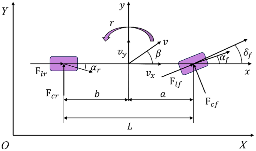
Single-track yaw-plane vehicle model.
According to Newton’s second law, the governing equations of motion are cast as:
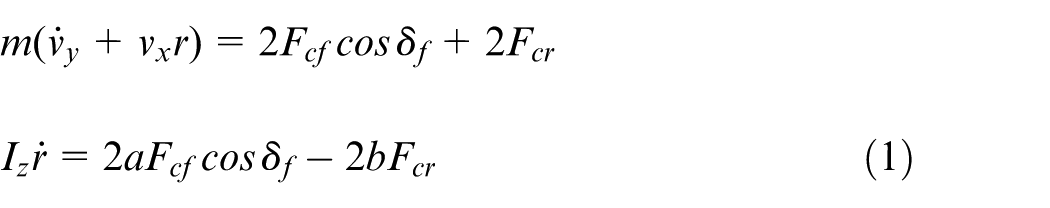
where m is vehicle mass, v x , v y , and r are longitudinal velocity, lateral velocity, and yaw-rate, respectively, δ f is front-wheel steering angle, I z yaw moment inertia, a and b denote distances from vehicle front and rear axles to its center of mass, respectively, F cf and F cr represent lateral force on front and rear tire, respectively.
To reduce the computational burden, this study adopts the linear relationship between tire lateral force and its slip angle. Thus, front and rear tire’s lateral forces are determined by:
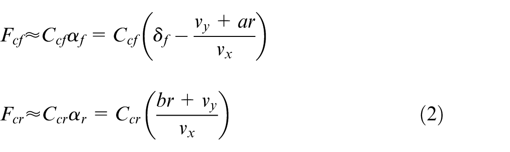
where C
cf
and C
cr
denote cornering stiffness of front and rear tires, respectively,
Considering the dynamic effect of human-driver’s direction control, the look-ahead preview distance is incorporated into the path-tracking error model, and the driver look-ahead path-tracking error model is shown in Figure 2. Since the vehicle is traveling along the desired path with a small heading angle, thus, tan(eφ) ≈ eφ, and the driver look-ahead path-tracking error model can be expressed as:
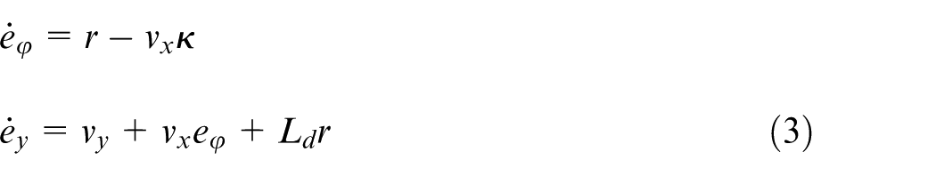
where
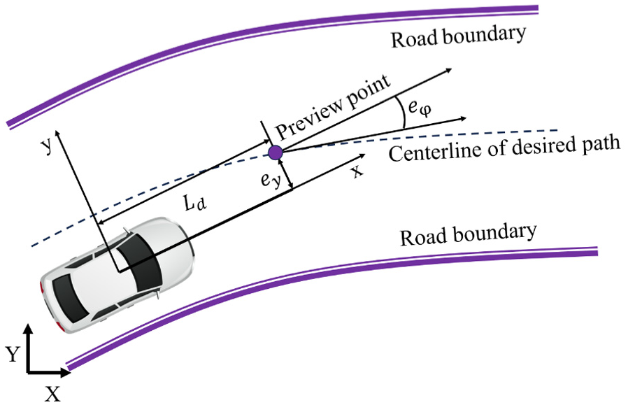
Driver look-ahead path-tracking error model.
Combining equations (1) to (3) leads to the linear state-space equation expressed by:

where
The cornering stiffness C
f
and C
r
of front and rear tire are affected by tire pressure, vertical load, and angle of lateral deflection.
38
In vehicle driving operations, especially steering, the vertical tire load varies within a range due to load transfer, and the cornering stiffness C
f
and C
r
are uncertain time-varying parameters, C
f
(k), C
r
(k). Thus, it may be assumed that
where
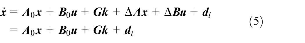
To apply the linear MPC to the path-tracking control, equation (5) needs to be discretized as:

where
Equation (6) is the discrete state-space equation of the vehicle model, which represents the actual system of the vehicle, while the nominal system of the vehicle can be expressed as:

where
CarSim vehicle model
The 3-D CarSim model comprises a rigid vehicle body, two suspensions, and four wheels. The motions considered involve the longitudinal, lateral, vertical, roll, pitch, and yaw motion of the body, as well as the vertical and spinning motions of each wheel. The nonlinear features of vehicle components, for example, suspensions and pneumatic tires, are mimicked in the model. Thus, this is a nonlinear 3-D vehicle model with 14-DOF.
In CarSim software, a symbolic multibody program, termed VehicleSim (VS) Lisp, is utilized to derive equations of motion for vehicle systems. 36 VS Lisp takes an input as the description of the 3-D vehicle model structure mostly in geometric terms, for example, the body DOF, point locations and the directions of force vectors. With the input information, VS Lisp generates equations of motion in terms of ordinary differential equations and produces a source code (e.g. C or Fortran) to solve them.
CarSim software consists of three key components: VS browser, CarSim database, and VS solver. The VS browser is a graphical user interface. The CarSim databases are used to choose vehicle structure templates, for example, dependent or independent suspension, and to define the system parameters, the tire-road interactions, the test maneuvers, etc. The VS solver is utilized to solve the derived governing equations of motion and to execute the defined simulations. The VS browser can also be applied to other applications, for example, incorporating the A-TRMPC controller to be designed in Matlab/Simulink to the 3-D CarSim vehicle model via an interface for co-simulation.
A-TRMPC controller design
In this section, firstly, the proposed design framework for the A-TRMPC controller is described. Secondly, the design of the conventional MPC controller is outlined. Then, the Tube-RMPC design is presented. Finally, the A-TRMPC design is introduced.
Design framework
The A-TRMPC controller design is formulated as a bi-layer optimization problem solved offline. The proposed design framework is shown in Figure 3. In the top layer, a Quantum Particle Swam Optimization (QPSO) search algorithm is selected to coordinate the design criteria considering the specified constraints; in the bottom layer, the A-TRMPC controller designed in Matlab/Simulink is integrated with the nonlinear 3-D vehicle model generated in CarSim software to fabricate a virtual autonomous vehicle. In the design optimization, the prediction horizon (
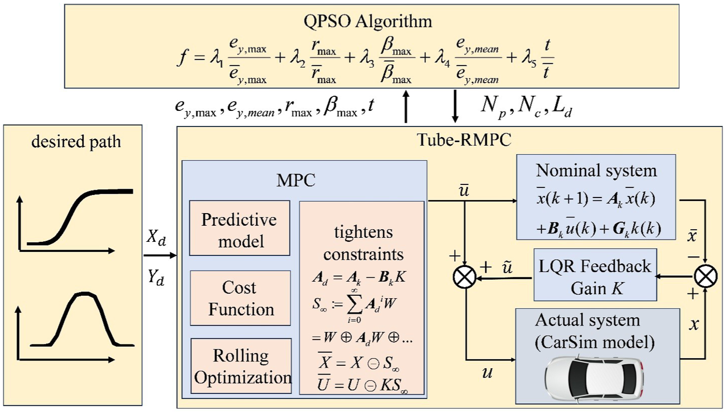
Proposed A-TRMPC controller design framework.
The QPSO algorithm is an improved version based on a conventional particle swarm optimization (PSO).
40
The QPSO can perform global searches in the search space and maintain a certain degree of diversity during the search process to avoid falling into local optimal solutions. As shown in Figure 3, the QPSO algorithm is pre-set with multiple sets of design variables, that is,
Over the testing maneuver, the MPC controller drivees the vehicle tracking the reference course as the reference path; the controller applies future control actions to the nominal system based on the current vehicle state to predict the future state of the vehicle so that the vehicle follows the desired path. The MPC solver calculates the nominal control sequence,
The LQR is a well-known optimal control technique, which is widely used to design state feedback controllers.41,42 To reduce the state error between the actual system and the nominal system, the LQR feedback control is applied to the actual system together with the nominal control. The LQR control gain K is used to derive future state errors to construct a robust positive invariant set. Finally, the constraints of the nominal system are tightened to satisfy the constraints of the actual system. As shown in Figure 3, it is assumed that the desired path is determined by the path-planning module, and this study mainly focuses on path-tracking control. Thus, the path-planning module will not be further discussed.
MPC controller
In this study, all path-tracking controllers are designed based on the conventional MPC technique. Thus, the fundamental components of the MPC technique are outlined.
Cost function
In the MPC path-tracking control design, the cost function is formulated to optimize the controller’s decision at each time step and to make the vehicle follow the desired path as much as possible. The cost function is expressed as:
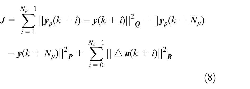
where
Constraints
Manipulating constraints is the main advantage of MPC path-tracking control. To ensure that the steering angle does not exceed the physical limits of the steering actuator, the maximum steering angle should be limited. In addition, limiting the steering angle rate ensures smooth control operation and prevents over-tuning. The constraints on the steering angle and the steering angle rate can be expressed as:


where δ f ,max and Δδ f ,max are the maximum value of the steering angle and the maximum value of the steering angle variation for one sampling step, respectively. Safe road transportation requires the controlled vehicle to operate in a feasible area without a collision. The lateral position error may be constrained so that the vehicle does not exceed the road boundary, and the heading error could be constrained to achieve accurate heading control and improve the performance of path tracking. The constraints on lateral position error and heading error are expressed by:


where e y ,max and eφ,max are the maximum values of lateral position error and heading error, respectively.
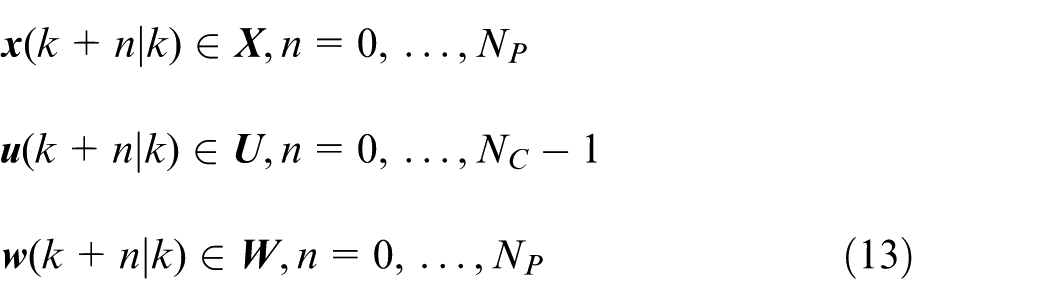
In summary, the constraints on the bounded uncertain disturbances in equation (6), the state variables, and the control variables of the actual system can be expressed as:
Tube-RMPC controller
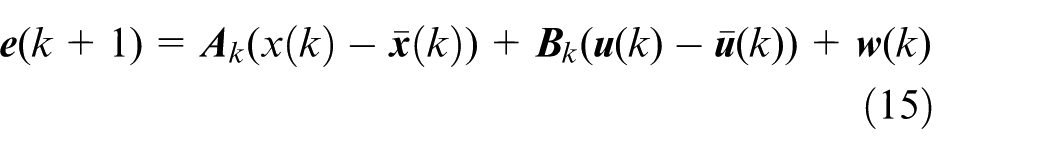
The nominal control for the nominal system is calculated by the MPC controller and is used to make the nominal system track the desired path. Due to the uncertain disturbances, the state error between the actual system and the nominal system can be expressed as:

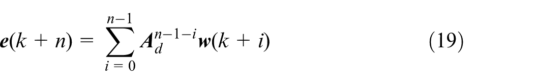
The state error at the next sampling step is:
To reduce the influence of uncertain disturbances, a feedback gain

Combining equations (14) to (16) leads to:
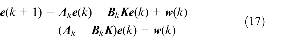
Let
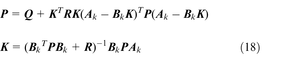
In the MPC controller, the nominal system state is equal to the actual system state at the current moment, that is,
There exists a robust positive invariant set
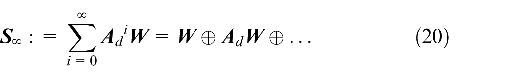
Equation (20) determines the invariant set
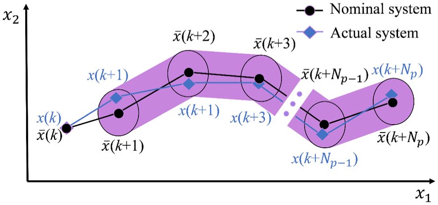
Schematic representation of state trajectory in prediction horizon.
To ensure that the actual system satisfies the constraints, the state, and control of the nominal system need to satisfy the following constraints:
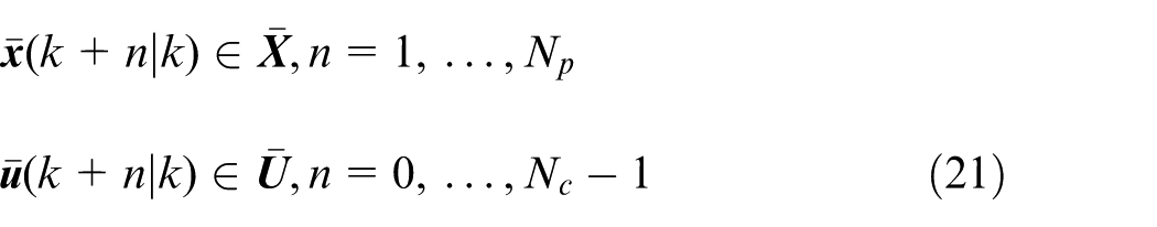
where
A-TRMPC controller
Built upon the Tube-RMPC controller designed in section 3.3, the A-TRMPC is designed by incorporating a variable look-ahead preview distance inspired by human-driver driving (see Figure 2) and considering variable prediction and control horizon. As shown in Figure 3, the A-TRMPC controller design is formulated as an optimization problem, in which the look-ahead distance
In this study, the QPSO 46 is used to optimize the look-ahead distance, prediction horizon, and the control horizon of the A-TRMPC controller. The QPSO is a metaheuristic search algorithm inspired by the quantum behavior of particles. It aims at improving the performance of Particle Swarm Optimization (PSO) by incorporating quantum mechanics principles. The QPSO is to explore the search space more effectively and avoid premature convergence. The position update expression of the quantum particle swarm is as follows:
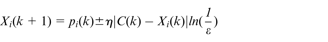
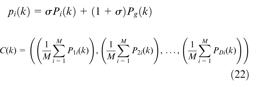
where D is the dimension of the search space (i.e. the number of design variables), M the population number of the particles,
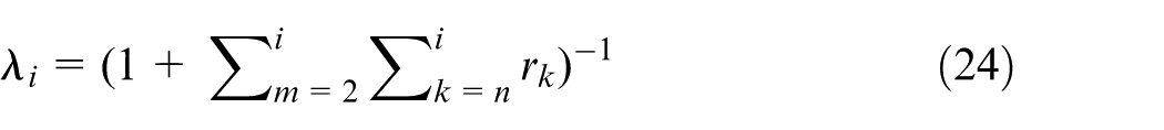
The QPSO is used to optimize the design variables (
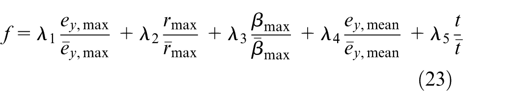
where λ
i
, i = 1,2,…,5, is the weighting factor, e
y
,max, rmax, βmax, e
y
,mean, and t denote the maximum lateral error, maximum yaw-rate, maximum slip angle, mean lateral error, and t the average computation time, respectively,
The fitness value of the objective function formulated in equation (23) is iteratively evaluated using the CarSim–Matlab/Simulink-based co-simulation shown in Figure 3. In each iteration, the data of e
y
,max, rmax, and βmax are acquired by taking the maximum values from their dynamic responses using the “max” function provided in Matlab/Simulink, while the measure of e
y
,mean is obtained by calculating the ratio of the integration of the corresponding response divided by the respective simulation time. By means of the above mathematical manipulation, the dimensionless value of each term of
where
Simulation results and discussion
To evaluate the proposed path-tracking control design method, this section presents the following research efforts: (1) examining the effect of the controller parameters, that is,
To validate the A-TRMPC, it is compared with the MPC and Tube-RMPC. For a rational and effective comparison, both the MPC and Tube-RMPC are also featured with the function of “look-ahead distance,” like the A-TRMPC. Thus, the MPC and Tube-RMPC are the co-called “tailored” controllers. For simplicity, hereafter, the tailored MPC and Tube-RMPC are termed the MPC and Tube-RMPC, respectively.
Effect of controller parameters on path-tracking control
To facilitate the examination of the effect of the controller parameters on the path-tracking performance of the vehicle, the MPC is selected. To conduct co-simulation, the vehicle and controller parameters take their nominal values listed in Tables 1 and 2, respectively.
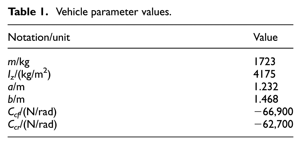
Vehicle parameter values.
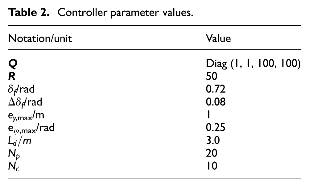
Controller parameter values.
For co-simulation, a testing path is designed to simulate the entry into a curve. The testing course is composed of two sections, the first section is a 25 m long straight line, and the second section is a curve with a curvature of 0.02 (1/m). The road adhesion coefficient is 0.85. In the co-simulation, the MPC intends to control the vehicle to follow the desired path at a speed of 60 km/h.
As listed in Table 2, the initial values for L d , N p , and N c are 3 m, 20, and 10, respectively. A sensitivity analysis for each of the three controller parameters is conducted. In each case, only one parameter is permitted to vary and the other two are fixed. Figures 5 to 7 visualize the impact on the path-tracking performance of the autonomous vehicle due to the look-ahead distance (L d ), prediction horizon (N p ), and the control horizon (N c ), respectively.
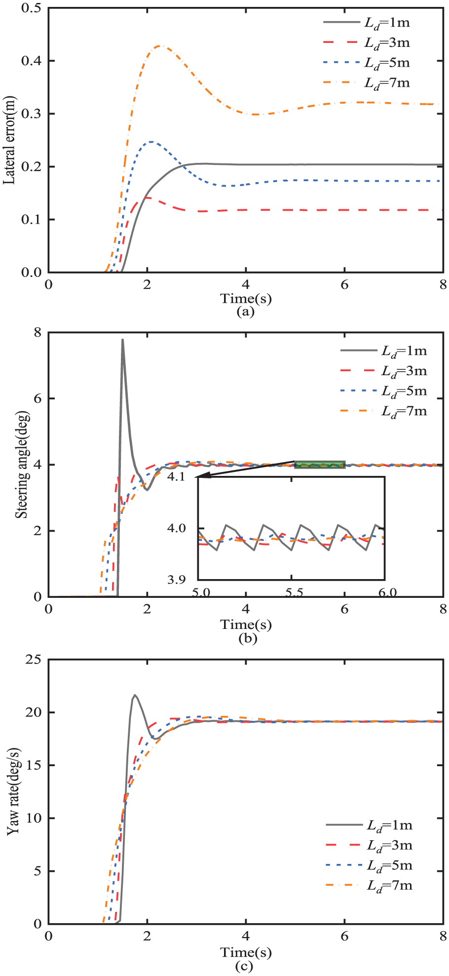
Effect of look-ahead distance L d on path-tracking performance: (a) lateral error; (b) steering angle; (c) yaw-rate.
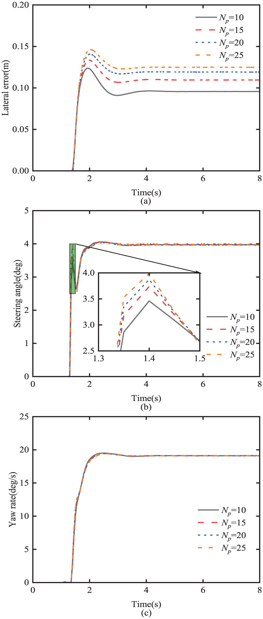
Effect of prediction horizon N p on path-tracking performance: (a) lateral error; (b) steering angle; (c) yaw-rate.
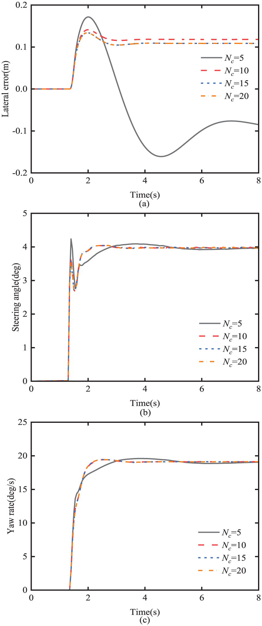
Effect of control horizon N c on path-tracking performance: (a) lateral error; (b) steering angle; (c) yaw-rate.
As shown in Figure 5(b), adding the look-ahead distance to the path-tracking error model causes the vehicle to steer early; the extent for steering in advance increases with the look-ahead distance L
d
. However, as seen in Figure 5(a), except for the case of
In the MPC controller designs, the larger the prediction horizon N p , the longer the future state of the system can be predicted, but it will reduce the control accuracy of the controller. As shown in Figure 6(a), the tracking error increases as N p increases. Unlike L d , the N p does not cause the vehicle to steer earlier. Figure 6(b) shows that the controllers all start controlling the vehicle steering at 1.3 s regardless of the different values of N p , and the steering angle increases rapidly within 0.05 s. The larger N p is, the larger the steering angle increment becomes, and the controller responds more quickly.
The control horizon N c determines the action range of the MPC future control quantities. As shown in Figure 7(b), a smaller N c makes the controller output not smooth enough and leads to insufficient control accuracy. Figure 7(a) illustrates the tracking error for a variety of N c , which decreases as N c increases. However, after N c is increased to 15, further increasing N c has no effect on the tracking accuracy of the controller. This is because the MPC controller applies only the first element of the control series to the controlled object during the control process.
In summary, it is found that the look-ahead distance, prediction horizon, and control horizon have important influences on the tracking accuracy and vehicle lateral stability control of the MPC path-tracking controller. Therefore, in this paper, the QPSO optimization algorithm is used to optimize the variables to attain their optimal values and improve the control effect of the controller.
Uncertain state disturbances for Tube-RMPC controller
To implement the Tube-RMPC controller introduced in subsection 3.3, the state disturbances, which result in the state trajectory tube, for example, the schematic representation shown in Figure 4, should be determined. In highway operations, a road vehicle frequently executes high-speed evasive maneuvers. To simulate a typical high-speed obstacle maneuver, we select the time-history of the vehicle front-wheel steering angle shown in Figure 8. Under the simulated maneuver with the road adhesion coefficient of 0.85 and nominal model parameter values, the maximum lateral acceleration of the vehicle may reach 0.45 g, where g is the gravitational acceleration.
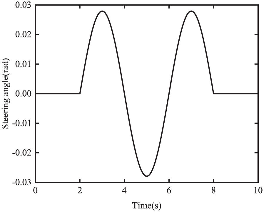
Front-wheel steering input for the testing maneuver for determining uncertain state disturbances.
As expressed in equation (4), the state variable vector of the vehicle model is denoted as
The uncertainty disturbances are attributed to the following sources: (1) modeling error between the nonlinear 3-D CarSim model with 14-DOF and the linear single-track yaw-plane model with 2-DOF; (2) external disturbances; and (3) model parameter uncertainties. To simulate the external disturbance, in the co-simulation testing, the road adhesion coefficient is set to randomly vary from 0.4 to 1.0, while the nominal road adhesion coefficient takes the value of 0.85. For mimicking model parameter uncertainty, the nominal vehicle mass for the linear model takes the value listed in Table 1, while the vehicle mass for the CarSim model varies stochastically from the nominal value by
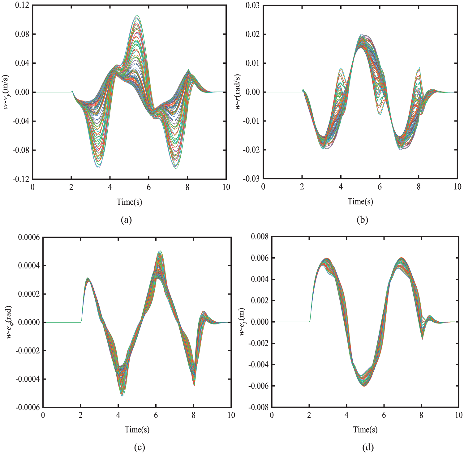
Simulation results of the one-step state error between the actual system and the nominal system: (a) lateral velocity error; (b) yaw-rate error; (c) heading angle error; (d) lateral error.
With the given uncertainty perturbations, the Tube-RMPC path-tracking control for the vehicle can be implemented.
A-TRMPC controller validation
To evaluate the proposed A-TRMPC path-tracking control design framework, two testing maneuvers are specified for CarSim–Matlab/Simulink-based co-simulations. The first scenario is a high-speed single lane-change (SLC) maneuver, where the road adhesion coefficient decreases from 0.85 to 0.3 at the longitudinal distance of 65 m along the testing course, and the vehicle speed is set to 100 km/h. This maneuver is intended to test the controller’s ability to cope with the sudden road adhesion coefficient change (i.e. an external disturbance) while the vehicle is performing a high-speed SLC for obstacle avoidance. The second scenario is a double lane-change (DLC) maneuver, where the roadway adhesion coefficient is 0.85, the vehicle speed is set to 100 km/h, and the vehicle mass is increased to 1.2 times of its nominal mass. This maneuver is intended to examine the controller’s ability to handle the variation of payload (i.e. a model parameter uncertainty) while the vehicle is executing a high-speed DLC for overtaking a preceding obstacle vehicle.
Three controllers are set up for the benchmark comparison. They are the MPC, Tube-RMPC, and the proposed A-TRMPC. In the benchmark comparison, for the MPC and Tube-RMPC, the controller parameters, that is,
Controller parameter values for the A-TRMPC.
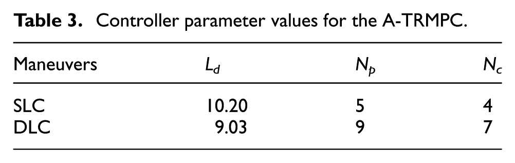
To illustrate the optimization efficiency of the QPSO algorithm, it is compared with a conventional PSO algorithm. 48 To this end, following the proposed framework shown in Figure 3, the two algorithms are independently applied to the design of the A-TRMPC controller. In setting up the two algorithms, the population number of the particles for both algorithms is set to 30 and the maximum number of iterations is 100. The two search algorithms are successfully implemented under the SLC and DLC maneuvers, and both individually find the same optimal values of the three design variables listed in Table 3.
Figure 10 shows the optimization processes of both the QPSO and PSO algorithms under the testing maneuvers, that is, SLC and DLC. As shown in the figure, under the SLC, the QPSO finds the fitness value of 0.5084 in the 12th iteration, while the PSO obtains the fitness value of 0.5297 in the 15th iteration; in the DLC, the QPSO finds the fitness value 0.7991 in the 15th iteration, while the PSO obtains the fitness value of 0.80231 in the 15th iteration. Compared to the PSO, the QPSO is faster and finds the solutions.
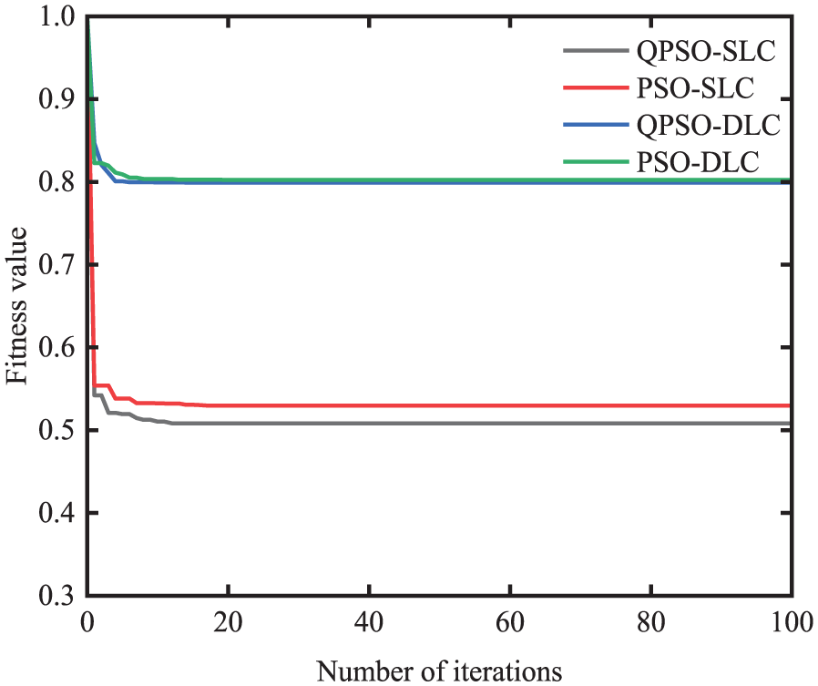
Performance comparison of QPSO and PSO algorithms.
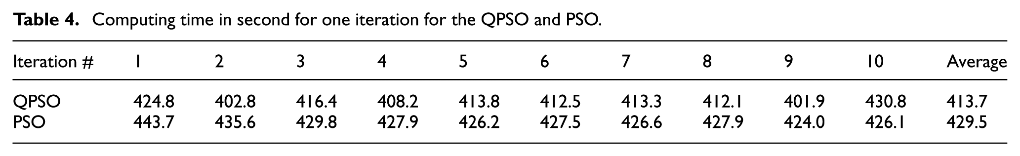
In this study, all calculations are carried out on a computer with a processor of Intel (R) Core (TM) i7-9750H CPU @ 2.59 GHz. Table 4 lists the computing time for each of 10 iterations for both the QPSO and PSO. For the former, the average computing time of one iteration is 413.7 s (6.89 min), while for the latter, the counterpart is 429.5 s (7.16 min), increasing by 3.8%. Once again, it confirms that the QPSO is more computationally efficient than the PSO.
Computing time in second for one iteration for the QPSO and PSO.
For simplicity, the following co-simulations are divided into two case studies: (1) SLC with road adhesion coefficient uncertainty and (2) DLC with vehicle mass uncertainty.
Case 1: SLC with road adhesion coefficient uncertainty
Figure 11(a) and (b) show the tracking tracks and heading errors of the three controllers under the SLC maneuver, respectively. After a longitudinal distance of 100 m, the three controllers show different magnitudes of overshoot. The A-TRMPC experiences the least overshoot and can be aligned with the left lane faster. This implies that among the three controllers, the A-TRMPC exhibits the best performance. Figure 11(c) and (d) display the lateral error and steering angle. The maximum lateral error for both the MPC and Tube-RMPC occurs around 4.3 s because the vehicle has a large overshoot in lateral displacement and cannot follow the desired path immediately after the lane change. The maximum lateral errors, Root Mean Square Error (RMSE) of lateral displacement deviation, the maximum yaw-rate, and the maximum side-slip angle are listed in Table 5. The maximum lateral error and the RMSE for the Tube-RMPC are smaller than their counterparts for the MPC, which indicates that the tracking accuracy of the Tube-RMPC is higher than that of the MPC. The maximum lateral error and RMSE for the A-TRMPC are 0.253 and 0.081 m, which are 61.95% and 61.06% lower than their counterparts for the MPC, respectively. Figure 11(e) and (f) show the yaw-rate and side-slip angle, respectively. The maximum values of the yaw-rate and side-slip angle of the A-TRMPC are reduced and approach 0 at 5.4 s. At this point, the vehicle has completed lane changing and begins to follow the left straight line.
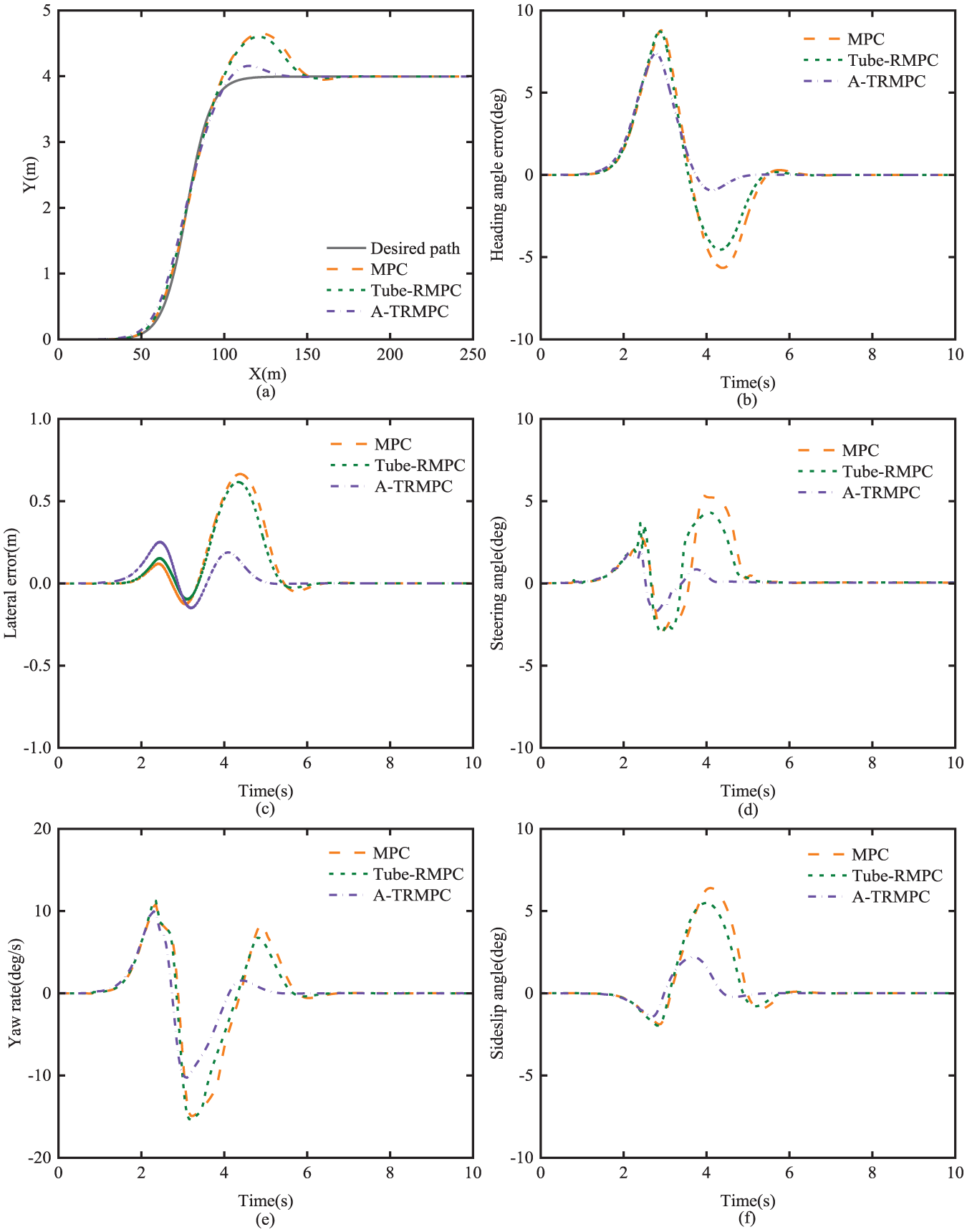
Path-tracking results under the SLC with road adhesion coefficient uncertainty: (a) tracking tracks; (b) heading error; (c) lateral error; (d) steering angle; (e) yaw-rate; (f) side-slip angle.
Path-tracking results under the SLC maneuver.
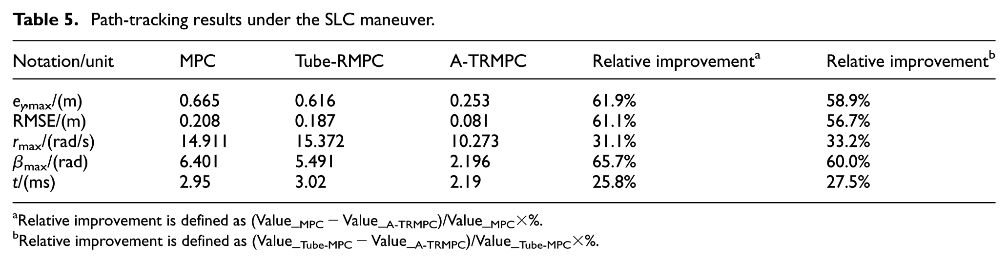
Relative improvement is defined as (Value_MPC − Value_A-TRMPC)/Value_MPC×%.
Relative improvement is defined as (Value_Tube-MPC − Value_A-TRMPC)/Value_Tube-MPC×%.
For the three controllers under the simulated SLC maneuver, Figure 12(a) and (b) show the computational time for each sampling time step and average computational time, respectively. The average computational times for the MPC and Tube-RMPC are 2.95 and 3.02 ms, respectively. With the same nominal values for N p and N c , compared with the MPC, the Tube-RMPC only takes 2.4% longer computational time. Thus, the Tube-RMPC outperforms the MPC in path-tracking with almost the same computational cost. The computational time for the A-TRMPC is 2.19 ms, which is 27.48% lower than its counterpart for the Tube-RMPC. Obviously, among the three controllers, the A-TRMPC behaves the best in terms of path-tracking and computational efficiency.
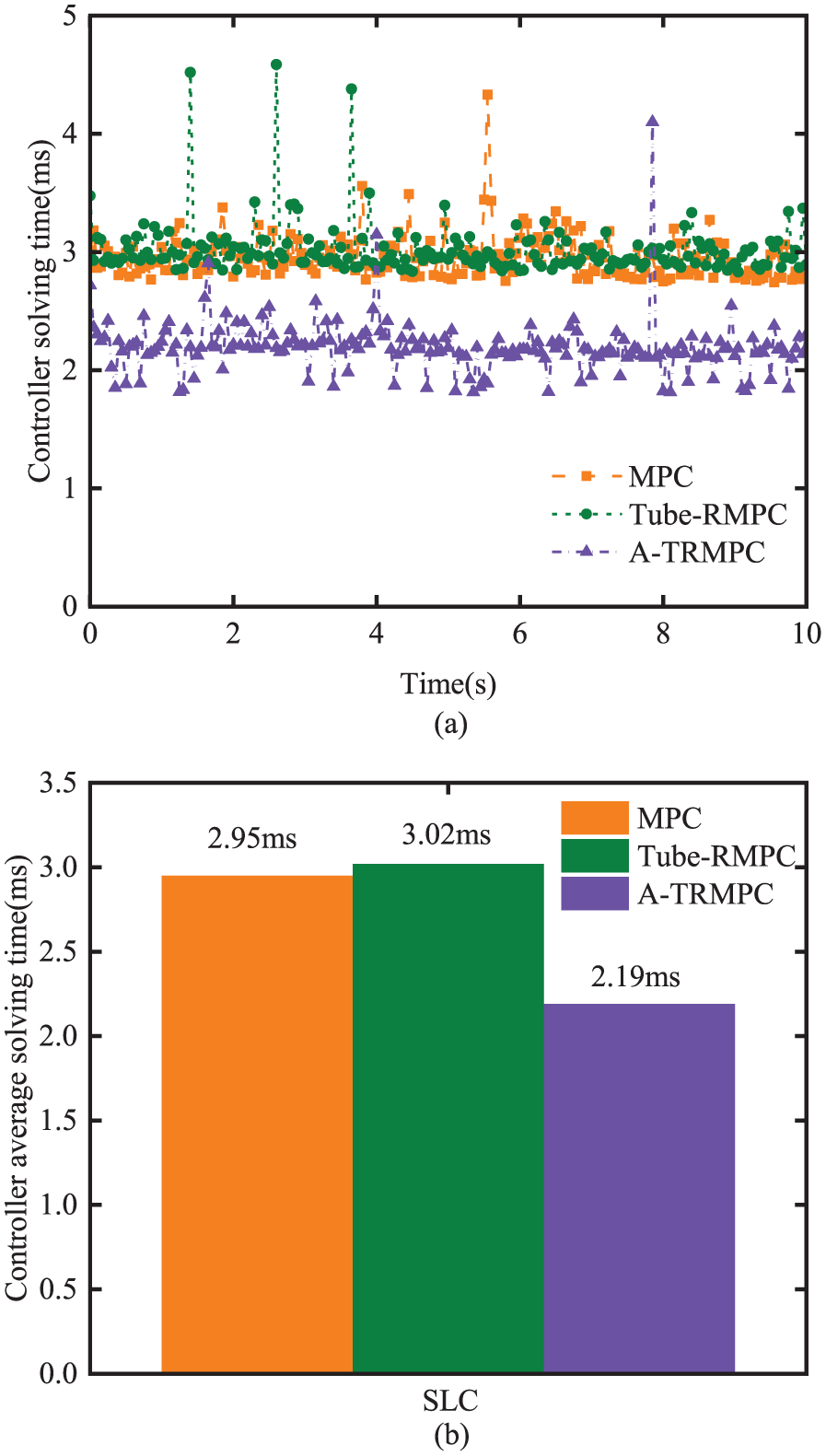
Computation time of the controllers under SLC maneuver: (a) computational time for each sampling time step; (b) average computational time.
Case 2: DLC with vehicle mass uncertainty
Figure 13(a), (d), (e), and (f) show the tracking trajectories, time-history of steering angle, time-history of yaw-rate, and the time-history of side-slip angle of the vehicle under the control of the three controllers over the DLC maneuver, respectively. A close observation discloses that among the three controllers, the A-TRMPC behaves the best, and the MPC performs the worst in terms of path-tracking, yaw-rate, and side-slip angle. Note that in terms of the performance measures of yaw-rate and side-slip angle, the smaller the peak values, the better the performance. Interestingly, the result seen in Figure 13(d) implies that among the three controllers, the A-TRMPC attains the best path-tracking control performance with the least steering effort, that is, the minimum steering angle peaks. Figure 13(b) and (c) illustrate the time-histories of the heading angle error and lateral error of the vehicle under the control of the three controllers under the DLC maneuver, respectively. The curves seen in these figures reveal the fact that among the three controllers, the A-TRMPC attains the least peak values, and the MPC causes the largest peak values in terms of heading angle error and lateral error. This evident further justifies the fact that among the three controllers, the A-TRMPC behaves the best and the MPC performs the worst in path-tracing control.
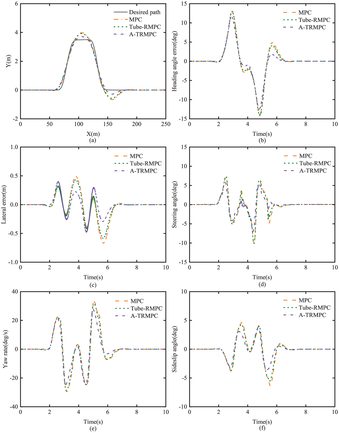
Path-tracking results under the DLC with vehicle mass uncertainty: (a) tracking tracks; (b) heading error; (c) lateral error; (d) steering angle; (e) yaw-rate; (f) side-slip angle.
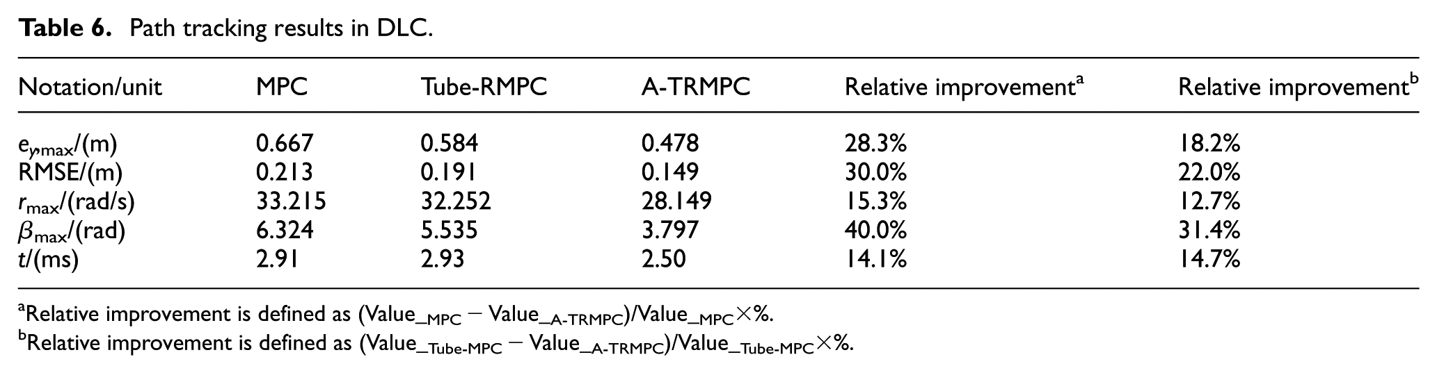
Table 6 summarizes the path-tracking performance measures of the vehicle under the control of the three controllers over the DLC maneuver. The maximum lateral errors of the MPC and Tube-RMPC are 0.667 and 0.584 m, respectively, and the RMSE of both the controllers are 0.213 and 0.191 m, accordingly. The maximum lateral error and RMSE of the A-TRMPC are 0.478 and 0.149 m, correspondingly, which are reduced by 28.3% and 30.0% compared with the MPC, respectively. Among the three controllers, the A-TRMPC achieves the least of the maximum yaw-rate and side-slip angle with the respective values of28.149 rad/s and 3.797 rad, reduced by 15.3% and 40.0% with respect to the counterparts of the MPC. This implies that A-TRMPC can best control the lateral stability of the vehicle among the three controllers.
Path tracking results in DLC.
Relative improvement is defined as (Value_MPC − Value_A-TRMPC)/Value_MPC×%.
Relative improvement is defined as (Value_Tube-MPC − Value_A-TRMPC)/Value_Tube-MPC×%.
Figure 14(a) shows the computational time at each sampling time for the three controllers. Figure 12(b) illustrates the average computational time of the three controllers. The average computational times for the MPC and Tube-MPC are 2.91 and 2.93 ms, respectively. The average computational time for the A-TRMPC is 2.50 ms, which is reduced by 14.7% compared to that of the Tube-RMPC.
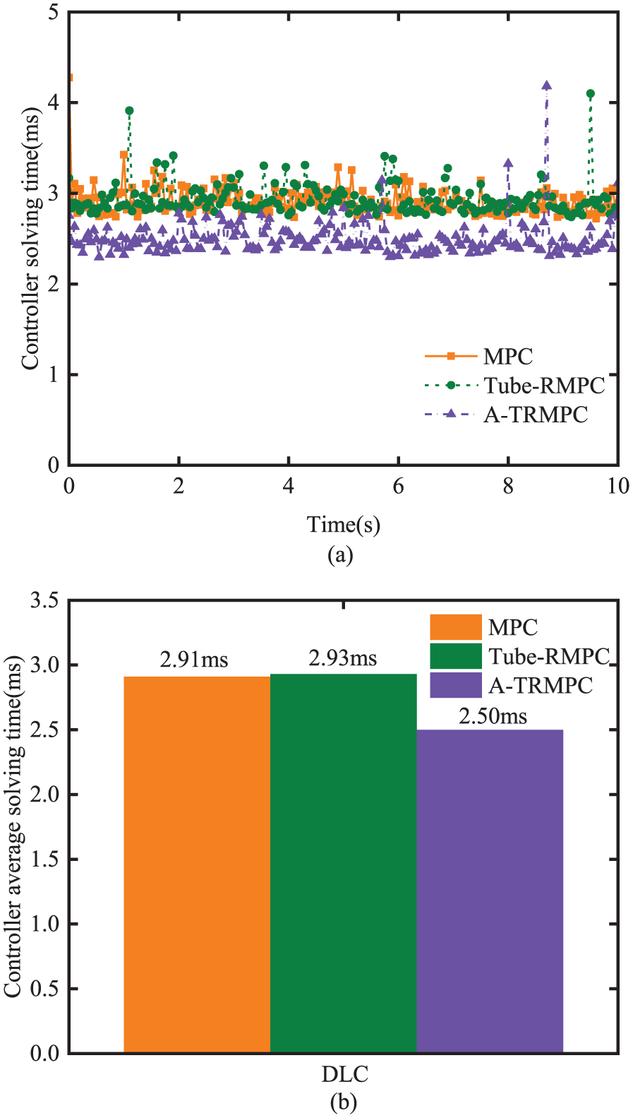
Computation time of the controllers under DLC maneuver: (a) computational time for each sampling time step; (b) average computational time.
Like the simulated SLC maneuver with road adhesion coefficient uncertainty, over the simulated DLC maneuver with vehicle mass uncertainty, the vehicle exhibits different path-tracking performance under the control of the three controllers. Among the three controllers, the A-TRMPC outperforms in terms of path-tracking performance and computational efficiency; compared with the MPC, the Tube-RMPC attains better path-tracking performance at almost the same computational cost.
The better path-tracking performance of the Tube-RMPC compared against that of the MPC is attributed to the following root cause. The Tube-RMPC is featured with the LQR feedback control based on the state error of the real system and the nominal system. Thus, the Tube-RMPC can deal with the modeling error, model parameter uncertainty, and the external disturbance, and make the vehicle have higher tracking accuracy. Among the three controllers, the A-TRMPC performs the best in path-tracking and computational efficiency, which stems from two essential features. Firstly, the A-TRMPC is built upon the Tube-RMPC, thus the former is also featured with the LQR feedback control based on the state error of the real system and the nominal system. Secondly, the A-TRMPC is featured with three adaptive controller parameters, that is, look-ahead distance, prediction horizon, and control horizon. As shown in Table 3, under different maneuvers, these three controller parameters should take different values to attain the desired path-tracking performance and computation efficiency specified in equation (23). These three parameters play different roles for the controller, and they interact on each other. Thus, optimizing them separately may not achieve optimal designs. The values for these parameters of the A-TRMPC are obtained using the QPSO search algorithm, which enables the parameters to be adaptive to different maneuvers. In both the testing maneuvers, the optimized prediction horizon and control horizon are smaller than the nominal ones, which contributes to the reduction of the controller computational time.
Conclusions
This paper proposes and develops an adaptive Tube-RMPC (A-TRMPC) controller design framework to improve the path-tracking performance of high-speed intelligent vehicles. To deal with model errors and external uncertain disturbances, a Tube-RMPC controller is devised using MPC and LQR techniques. The look-ahead distance is incorporated into the tracking error model. For the A-TRMPC, the three controller parameters, that is, the look-ahead distance, prediction horizon, and the control horizon, are treated as design variables, and they are optimized using a QPSO algorithm to improve the real-time performance of the controller.
To validate the proposed design method, the A-TRMPC is compared against the “tailored” MPC and Tube-RMPC using CarSim–Matlab/Simulink-based co-simulations, which are conducted to simulate a SLC and DLC maneuver at a vehicle speed of 100 km/h with roadway adhesion coefficient uncertainty and with vehicle mass uncertainty, respectively. Simulation results indicate that the proposed A-TRMPC improves the path-tracking accuracy and lateral stability of the vehicle with reduced controller computational burden.
In the near future, more external disturbances will be considered and applied to real vehicles to validate the proposed control strategy. In addition, the A-TRMPC will be compared with the state-of-the-art control algorithms, that is, min-max RMPC and stochastic RMPC.
Footnotes
Declaration of conflicting interests
The authors declared no potential conflicts of interest with respect to the research, authorship, and/or publication of this article.
Funding
The authors disclosed receipt of the following financial support for the research, authorship, and/or publication of this article: This research was financially supported by the Natural Science and Engineering Research Council of Canada (grant number RGPIN-2019-05437).