
Abstract
The thermal errors of a motorized spindle are seen as a source of significant errors in computer numerical control (CNC) machine tools, and motion errors, geometrical errors, among others, that are consequences of the thermal errors in the spindle. A predictive model of the thermal errors of a motorized spindle is proposed using a loading method based on heat flux. At first, a finite element model for the steady-state and transient thermal-structure coupling analysis of a motorized spindle is established, in which the loading method based on heat flux is adopted to assign the total amount of heat to the ball, an inner race, and an outer race of angular-contact ball bearing proportionally. The response values of sample points are obtained by simulation, and then a response surface model for the prediction of the steady-state elongation of the spindle thermal deformation under the influences of four factors including rotational speed of a bearing, coolant temperature, ambient temperature, and preload is constructed. The simulation and experimental results indicate that predictive error of the steady-state elongation of the spindle thermal deformation is only 3.81 μm, and the thermal equilibrium time in the transient thermal-structure coupling analysis is almost same to the experimental result. The response surface model can predict steady-state errors arising from the changes in working conditions and corresponding changes of the spindle.
Introduction
The errors incurred by thermal deformation can impair the machining accuracy of high-speed and high-precision machine tools to a significant extent. For precise machine tools, thermal errors account for 40%–70% of the total errors. 1 The thermal error of a motorized spindle, as the core component of a machine tool, is one of the major factors affecting the overall thermal error of the machine tool. Therefore, studying the prediction and compensation for thermal deformation of the motorized spindle is important when trying to improve the machining accuracy of machine tools.
The modeling and prediction methods of thermal errors mainly include empirical and theoretical modeling of thermal errors. According to whether considering the thermoelastic effect or not, the empirical models of thermal errors can be further divided into the quasi-static model and the dynamic model. 2 The theoretical modeling methods of thermal errors include the finite element method, a thermal network method, and a lumped mass method. At present, the finite element method is an effective approach for studying thermal errors. By applying accurate thermal boundary conditions and corresponding analytical settings to an appropriately simplified finite element model, the finite element simulation software can perform iterative computation based on the variational principle, weighted residual methods, and the thermodynamic temperature equilibrium equation. In this way, the temperature field and the thermal deformation field of the model can be obtained. Li et al. employed ANSYS software to study influences of the air-gap state between the stator and rotor of a motorized spindle on the steady-state thermal deformation of the motorized spindle. 3 Xu and Fan combined the finite element method and digital twinning to improve the simulation accuracy for thermal errors of a motorized spindle by mapping and modifying the thermal boundary conditions including the thermal contact resistance. 4 Deng et al. established a coupling analysis model for the spindle–vertical column system of a machine tool using the finite element software and obtained key thermal properties of the model, including the thermal equilibrium time. 5 Fang and Xiang incorporated finite element analysis with deep learning and convolutional neural networks to model and predict the thermal errors of a motorized spindle under complex conditions. 6 Naumann et al. proposed a tailored implicit–explicit multi-rate, high-order time-stepping method for real-time and accurate simulation of transient thermal deformation of the finite element model of machine tools. 7 Liu et al. used ANSYS to establish a finite element model of a spindle and studied the temperature, thermal deformation, and rotational accuracy at different rotational speeds. 8 Li et al. optimized the convective heat transfer coefficient based on the inverse heat conduction theory and numerically simulated the temperature field and thermal errors of the motorized spindle in ANSYS. 9 By combining the finite element model and experimental data, Zhang et al. optimized the convective heat transfer coefficient based on the temperature measurement data on the surface of the spindle and constructed a high-accuracy predictive model of temperature rise for the motorized spindle. 10 Fan integrated the finite element method and experimental method to establish an on-line monitoring program, which is used for real-time prediction of the thermal deformation of the motorized spindle of a machine tool. 11 Based on the finite element analysis method and information theory for the thermal errors of machine tools, Li and Ying optimized the locations of temperature-measurement points of machine tools. 12 Liu et al. used the hybrid response surface method to optimize the multi-objective parameters of the boundary conditions such as thermal load, convective heat transfer coefficient and thermal contact resistance, thereby improving the accuracy of simulation of the transient thermal characteristics analysis model of a ball screw feed drive system. 13 Jae-Seob Kwak used the response surface method to evaluate the influences of grinding parameters including wheel speed, table speed, depth of cut, and grain size on the geometric error, established a second-order response surface model of the geometric error and determined the optimal grinding conditions when the geometric error was minimized. 14 Uhlmann and Hu presents a 3D FEM model to predict the thermal behavior of a high speed motor spindle. This model allows a transient simulation which considers complex boundary conditions like heat sources as well as contact and convective heat transfer between spindle parts. 15 Chen et al. calculated the laminar forced convection heat transfer coefficient of the machine tool spindle under different working conditions, which provides a basis for heat transfer correction. 16
The aforementioned studies evaluated thermal properties of a motorized spindle from different perspectives including correction of the convective heat transfer coefficient, optimization of the time step for transient analysis, and layout of temperature-measurement points based on the ANSYS finite element simulation software. Despite this, the loading mode based on the heat generation rate is generally used when applying thermal boundary conditions to the bearings, which are one of the heat sources of a motorized spindle. That is, a bearing is used to simplify the internal heat transfer behavior and various components are assumed to be heated uniformly. However, Burton and Staph proposed in their research on the angular-contact ball bearings that one-quarter of the total heat generated in a ball bearing under a high centripetal force is transferred to the outer race, another quarter to the inner race, and the rest to the balls. 17 This finding means that the heat generated by the balls is much higher than that of the inner and outer races in practice. What’s more, in the Ansys Workbench, when the heat generation rate load is loaded on the bearing model, the bearing as a whole is selected as an individual feature and then the corresponding value of heat generation rate thermal load is loaded. This method ignores the temperature gradient of the bearing, so it can not accurately describe the actual heating situation of each component in the bearing, leading to large error in the simulation results. But when the heat flux load is loaded to the bearing model, the inner ring, outer ring and the surface of each ball are selected one by one as the surface characteristics, and then the corresponding heat flux thermal load is precisely loaded on these surface characteristics according to the actual heat distribution law, the friction heat generation of each surface of the parts of the bearing can be described more precisely. Furthermore, the thermal load applied based on the rate of heat generation is generally used to simulate heat generation via chemical reactions and electrical heat generation, 18 which are different from the heating mode of stators and rotors. Heat generation in a bearing mainly results from frictional heating between contact surfaces. Therefore, applying thermal loads based on the rate of heat generation in simulations is probably less realistic.
For the finite element model of a motorized spindle in a three-axis computer numerical control (CNC) machine tool, the total amount of heat is accurately distributed to the balls, inner race, and outer race of angular-contact ball bearing sets when applying the heating boundary conditions to the bearing sets to the front and rear of the motorized spindle. This assumed relatively shallow heat penetration of angular-contact ball bearings as per theoretical research on dry torque. Then, the steady-state and transient temperature fields and the thermal deformation are simulated and studied by applying loads based on heat flux. The results are then compared with those using the traditional loading mode based on the rate of heat generation. Moreover, a response surface model for predicting the thermal elongation of the spindle is established. Through the response surface analysis, the parameters of the bearing speed, coolant temperature, ambient temperature, and preload are optimized to control the thermal elongation of the spindle. Finally, the temperatures at key points for the thermal errors of the motorized spindle and the thermal elongation at the end of the motorized spindle are measured by conducting experiments on thermal properties of the motorized spindle. This result verifies the effectiveness of the loading mode based on heat flux and the research improves the accuracy of finite element prediction for the thermal errors of the motorized spindle. The objective of this paper is to accurately predict and model the thermal deformation of motorized spindle, due to the complexity of the motorized spindle system and the measurement error of detection equipment, the prediction accuracy of this model has been improved, the thermal contact resistance between parts is ignored and the geometric model of the motorized spindle is simplified in this paper. and there is still room for further improvement compared with the real thermal deformation of the motorized spindle.
Generation mechanism of thermal errors and calculation of heat generation and heat transfer
Generation mechanism of the thermal errors of a motorized spindle
The thermal errors of a motorized spindle are the result of superimposition of thermal deformation of various components therein. The temperature field changes with time; however, different levels of thermal stress occur to various components of the motorized spindle in the varying temperature field because of discrepancies among the various components in the coefficient of thermal expansion, thermal conductivity, and other material parameters. As a result, various components are thermally deformed to different extents. As shown in Figure 1(a), the changes in the temperature field and the thermal deformation are both hysteretic and influences of various factors are characterized by the thermal errors at the end of the motorized spindle, and the actual picture of the experimental motorized spindle is shown in Figure 1(b).
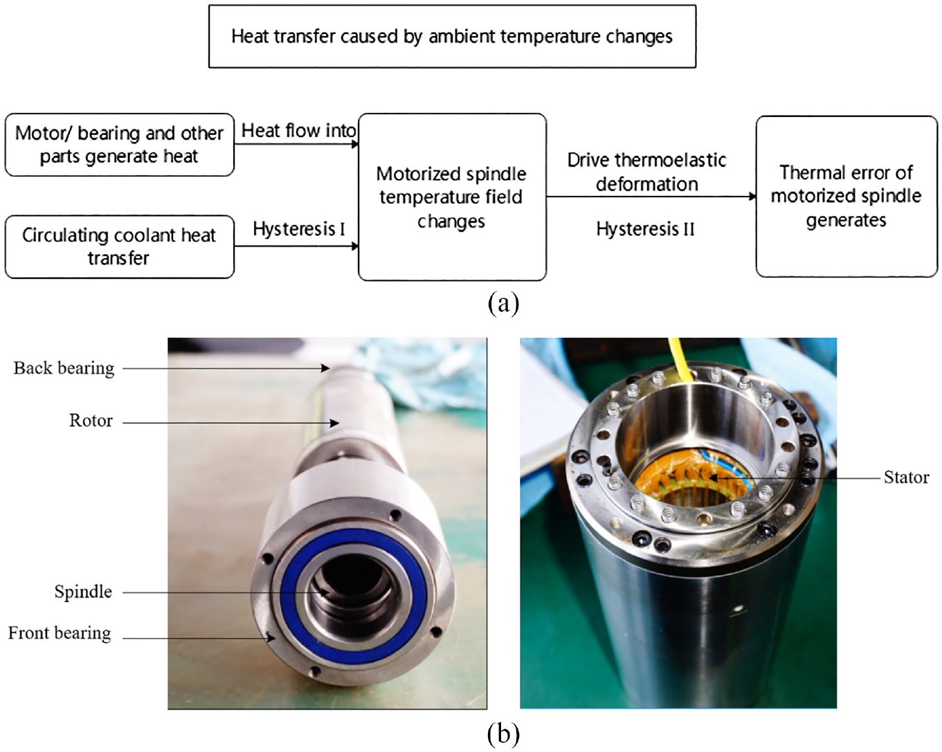
(a) Mechanism of the thermal errors of a motorized spindle and (b) the actual picture of the experimental motorized spindle.
Calculation of heat generation in a motorized spindle
Calculation of heat generation in angular-contact ball bearings
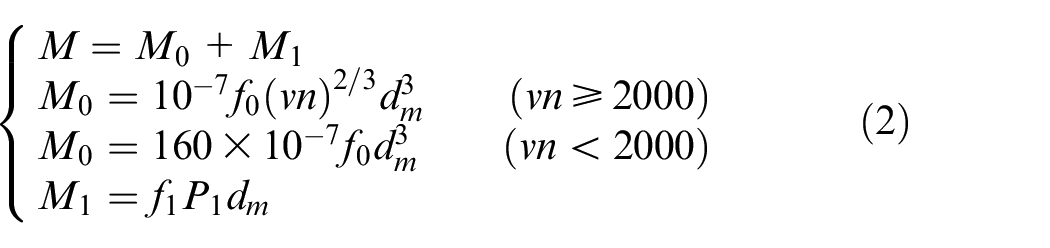
Heat is generated because of friction between balls and inner and outer races when a bearing is rotated at a high speed. The heat generation is mainly related to the rotational speed and friction torque can be calculated using the following equation:

where
By referring to the method in previous research, 19 the friction torque of the bearing is divided into two parts: the friction torque induced by applied loads and the friction torque caused by the viscosity of lubricants. That is, the equation for the friction torque of the bearing under conditions of moderate load, normal lubrication, and moderate angular velocity is expressed as
where
Taking the angular-contact ball bearing in front of the motorized spindle as an example, the heat flux on the surface of various components therein is deduced using the following equation:
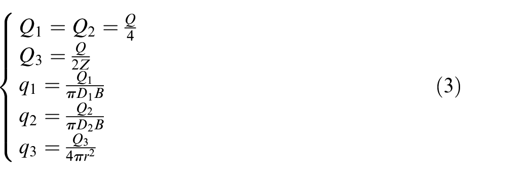
where
Calculation of heat generation at the stators and rotors
The loss and heat generation of a motor mainly comprise the mechanical loss, magnetic loss, and electrical loss, each of which has a corresponding theoretical formulation; however, calculation of the power loss using the theoretical formula requires the user to determine many parameters. Therefore, the power conversion method that is simple and feasible in the engineering practice is used here to estimate the power loss 20 :
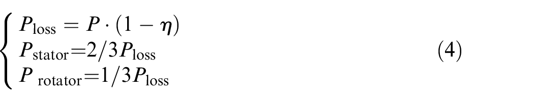
where P and ɳ denote the rated power of the motor (W) and efficiency of the motor, respectively;
Supposing that the power loss is completely converted to heat, then heat generation rates of the stators and rotors can be calculated using the following equation:
where
Analysis and calculation of heat transfer in the motorized spindle
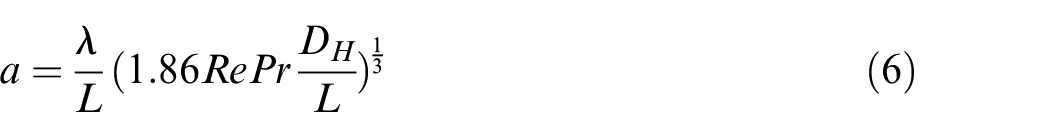
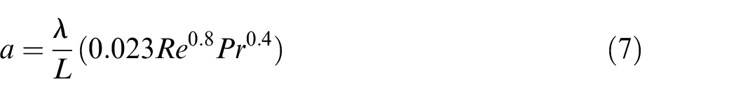
During heat convection between various components of the motorized spindle and the fluids, the stators and bearings have large convective heat transfer coefficients with the coolant oil and their heat is constantly absorbed by circulating coolant oil in the spiral cooling jacket at the fluid–solid interface. The different flow conditions of coolant oil in the cooling channels lead to different convective heat transfer coefficients, making it necessary to determine the flow condition of cooling water at first based on the Reynold’s number. The convective heat transfer coefficient between the stator and the cooling oil, as well as that between the bearing and the cooling oil can be confirmed by equations (6)–(8) 21 :
When Re <2000, the laminar region is
When 2000 < Re < 10,000, the transition zone between the laminar flow and turbulent flow is
When Re > 10,000, the turbulent region is
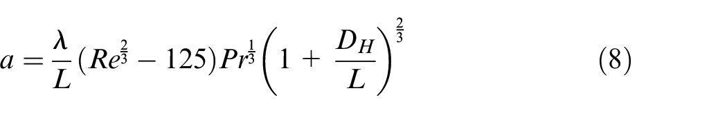
where Re is the Reynold’s number; Pr, DH, and λ represent the Prandtl number, equivalent diameter (m), and thermal conductivity (W/(m2·K)) of the coolant, respectively; L is the geometric feature length of the heat transfer surface (m).
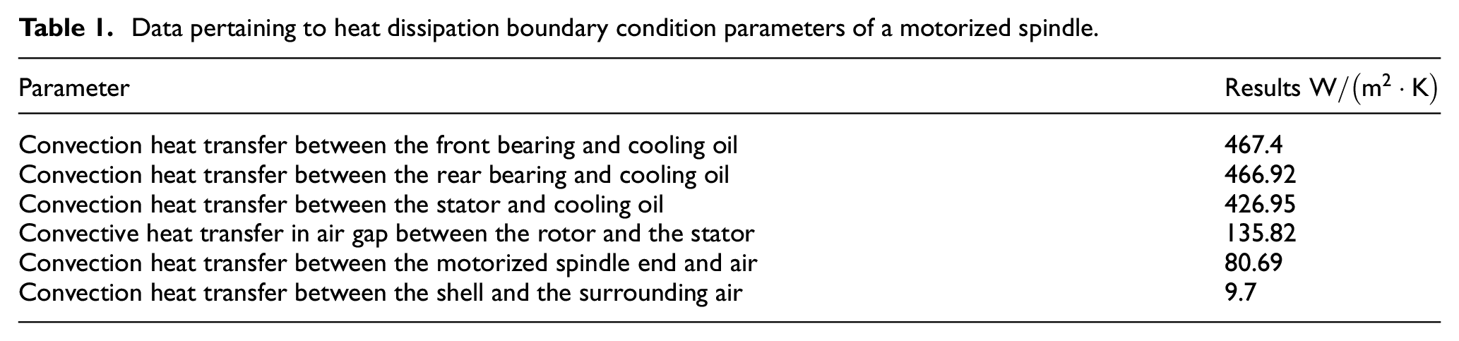
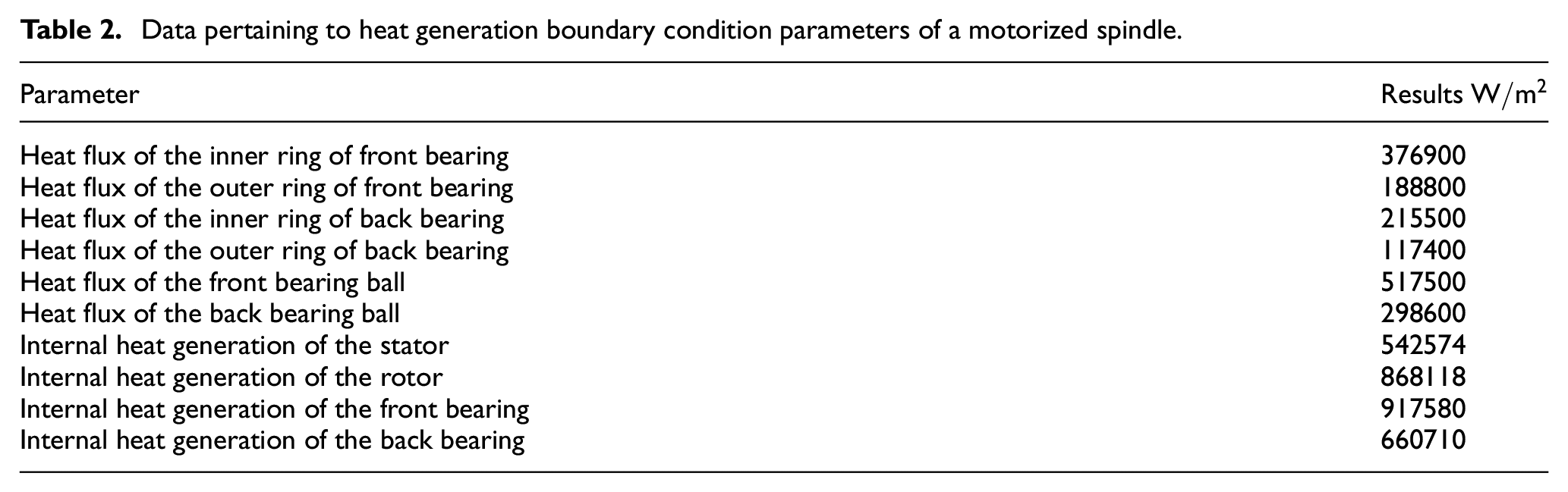
The convective heat transfer coefficients of other components in the motorized spindle can be calculated by using the theoretical or empirical formulas proposed elsewhere.22,23 The convective heat transfer coefficients are summarized in Table 1. The heat generation boundary condition parameters are summarized in Table 2.
Data pertaining to heat dissipation boundary condition parameters of a motorized spindle.
Data pertaining to heat generation boundary condition parameters of a motorized spindle.
In addition, according to relevant research conclusions, 24 Compared with other types of boundary conditions, thermal radiation and contact thermal resistance have little influence on the thermal deformation of motorized spindle, so these two types of boundary conditions are ignored in this paper when modeling.
Finite element simulation and response surface analysis of the thermal errors of the motorized spindle
Finite element model of the motorized spindle
The 7008C/7006C-2RZ-P4 angular-contact ball bearings are set at the two ends of the motorized spindle in the present research. After being appropriately simplified, the geometric model is imported in ANSYS Workbench and material properties of each component are defined. In addition, contact pairs are established between adjacent components in the motorized spindle. Therein, the friction coefficient between (inner and outer) races and balls is set to 0.2, and other components without relative motion are bonded. Because stators and rotors have regular geometric shapes, their meshes are mainly generated with hex-dominant elements and automatic meshing is performed for other components. The element size is 3 mm (edge length) while areas with large temperature gradients are refined using an element size of 2 mm. The generated mesh is illustrated in Figure 2.
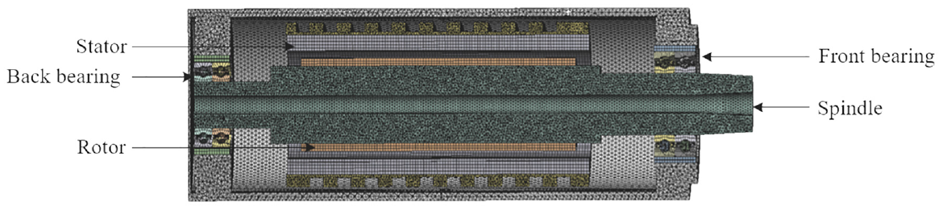
The finite element meshing model of a motorized spindle.
Establishment of a steady-state thermal model
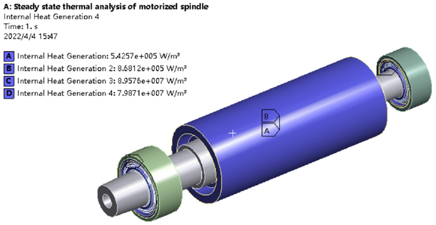
Steady-state thermal analysis is conducted on the motorized spindle in ANSYS Workbench under the following initial conditions: rotational speed of the motorized spindle of 10,000 rpm, an ambient temperature of 22°C in the experiment, and the coolant temperature of 24°C. The convective heat transfer coefficients of various components of the motorized spindle summarized in Table 1 are initially applied to the corresponding locations. Then, thermal boundary conditions are applied to two identical finite element models under two conditions: one is the loading mode based on heat flux to the angular-contact ball bearings in front and rear of the motorized spindle; and the other is that based on the rate of heat generation. In these two modes, the thermal load is applied to the stators and rotors both based on the rate of heat generation (Figures 3 and 4). Each letter represents the surface of a part or the body of a part, and the number on the left represents the amount of load being loaded on the part.
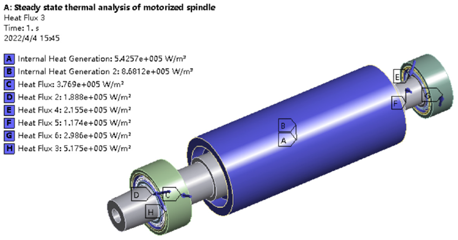
The loading mode based on heat flux.
The loading mode based on the rate of heat generation.
The steady-state temperature field and the deformation field obtained by solving the finite element models under the two loading modes are displayed in Figures 5 to 8.
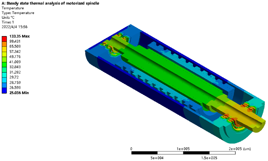
Steady-state temperature field under heat flux load.
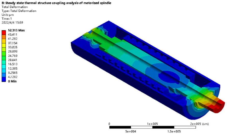
Thermal deformation under the heat flux load.
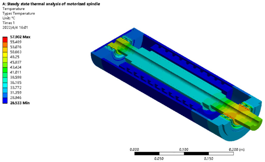
Temperature field under rate of heat generation load.
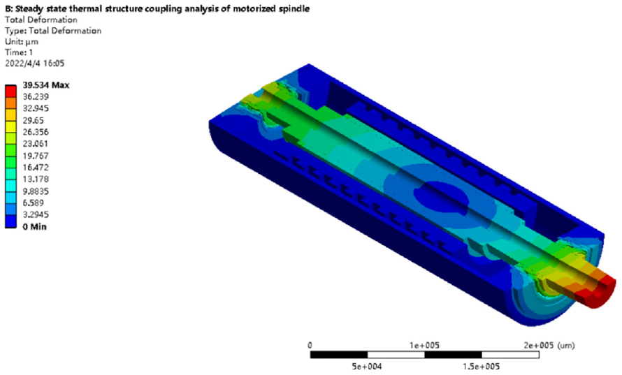
Thermal deformation under rate of heat generation load.
Figures 5 and 7 show that the highest temperature is found at the balls of the angular-contact ball bearing in front of the motorized spindle if the thermal load is applied based on heat flux; while it occurs at the inner race of the front angular-contact ball bearing when the thermal load is applied based on the rate of heat generation; this is because, in the former loading mode, heat is distributed such that the heat is the sum of that of the inner and outer races of the ball bearing and therefore heat is mainly concentrated within the balls, and this is more close to the actual heat generation of the internal parts of the bearing. In addition, thermal contact resistance is also present between balls and inner and outer races, which contributes to the relatively high local temperature of the balls and the significant temperature gradient across the inner and outer races. When the thermal load is applied based on the rate of heat generation, the overall temperature gradient across the ball bearing is low because the actual heating conditions of various components of the ball bearing are simplified and heat is regarded as being uniformly distributed in the angular-contact ball bearing. But in fact, the internal parts of the bearing are not uniformly heated, Therefore, it is inevitable that there will be a relatively large error when using this loading method as the boundary condition for simulation.
Transient thermal analysis of the motorized spindle
ANSYS is used to establish a transient thermal analysis system of the motorized spindle and the mesh model and material parameters used in the steady-state thermal analysis module are transferred to the transient thermal analysis module. In the transient thermal analysis, the simulation time, time step, and number of time steps are separately set to 14,400 s, 100 s, and 144 to simulate the whole process from the cold state to thermal equilibrium of the motorized spindle. Here, only the cloud picture for simulation at some moments in the loading mode based on heat flux is displayed. Figure 9 shows the cloud picture for the temperature field in the 30th time step after operating the motorized spindle for 3000 s, which is approximately the simulation time to reach the thermal steady state of the spindle.
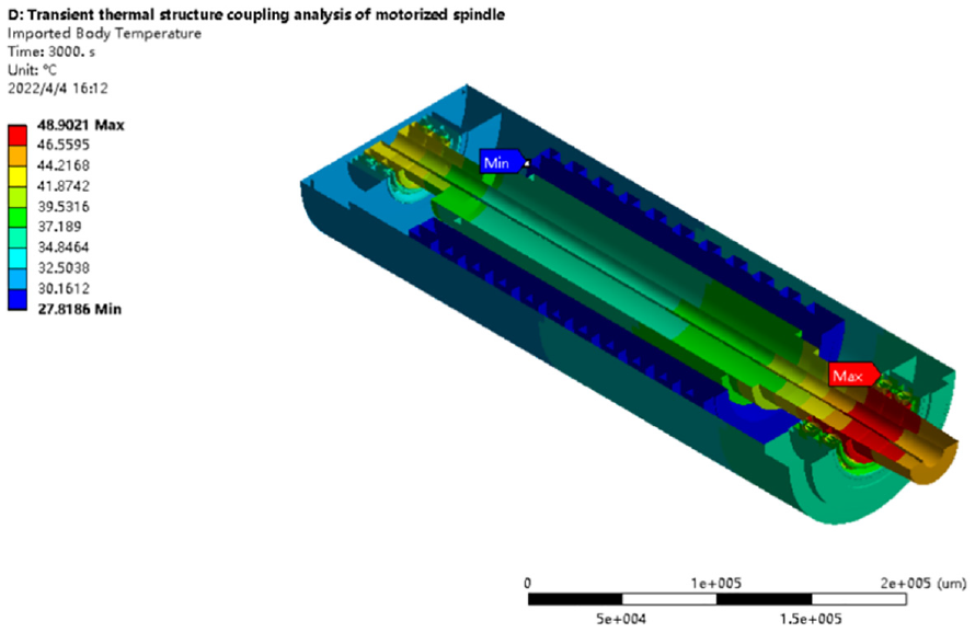
Temperature field after running for 3000 s.
The temperature fields at 144 time points are all imported into the structural analysis module of ANSYS and appropriate constraints are applied. The cloud pictures for thermal deformation corresponding to the temperature fields are solved. Figure 10 illustrates the cloud pictures for the overall thermal deformation and thermal deformation in the X, Y, and Z-directions after operating the motorized spindle for 3000 s. These cloud pictures show that thermal deformation of the motorized spindle mainly occurs in the axial direction, and the maximum axial thermal deformation is 50.86 μm; the thermal deformation in the X and Y-directions is relatively small, with the maximum values being 13.67 and 13.23 μm, respectively.
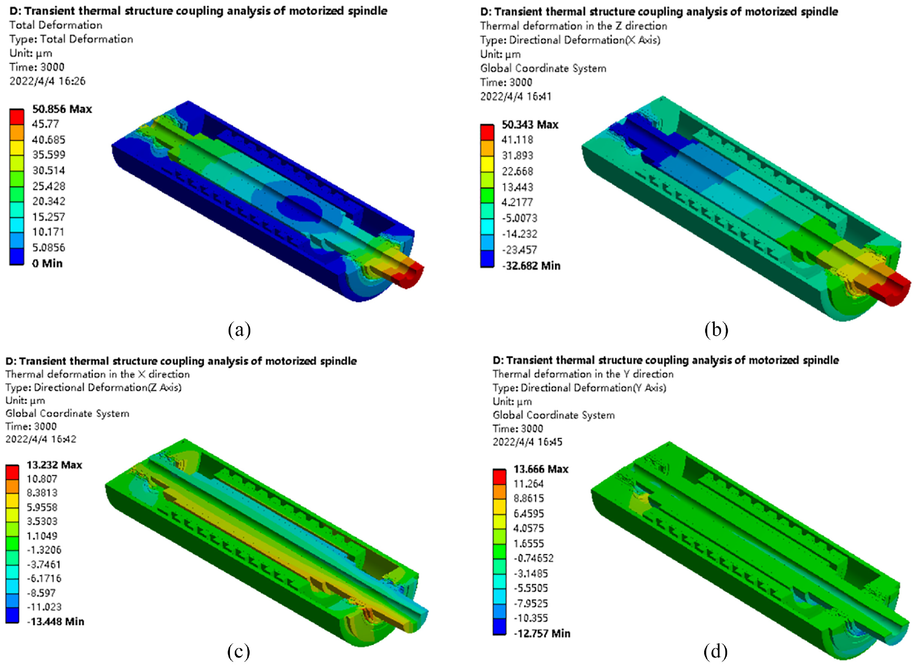
Thermal deformation after running for 3000 s: (a) total thermal deformation, (b) thermal deformation in the Z-direction, (c) thermal deformation in the X-direction, and (d) thermal deformation in the Y-direction.
Furthermore, the spindle and the front angular-contact ball bearing in the motorized spindle are taken as objects for analysis. After resetting, thermal deformation of each component can be observed (Figures 11 and 12). The thermal deformation of the spindle is shown to be concentrated at the end thereof, while that of the angular-contact ball bearing set is mainly concentrated in the inner race, with the maximum thermal deformation of 33.84 μm.
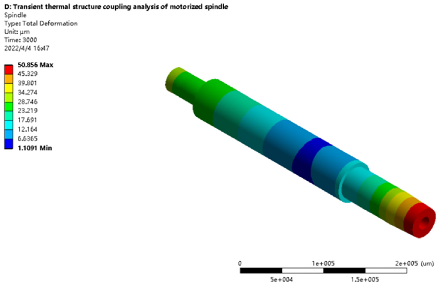
Thermal deformation of the spindle.
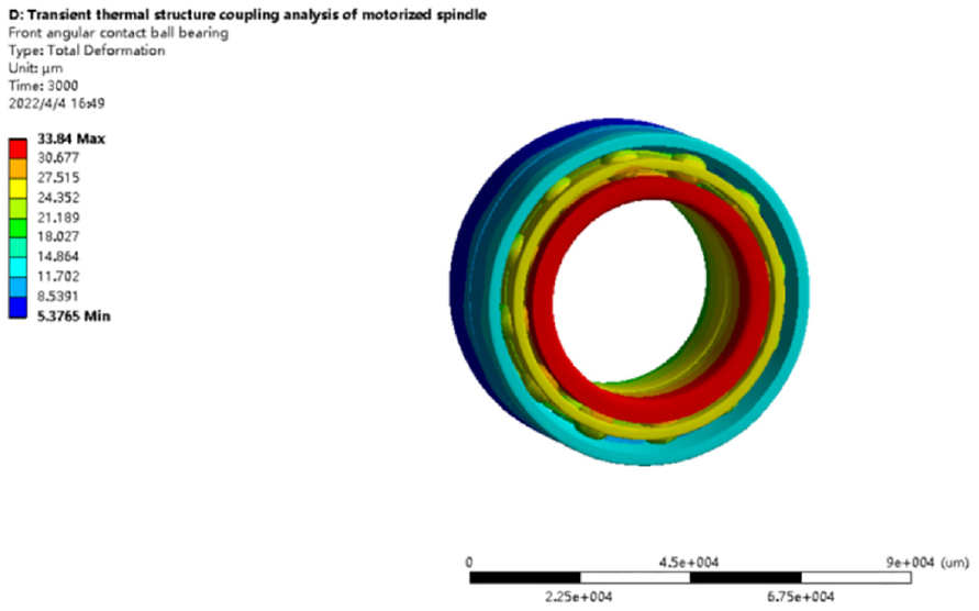
Thermal deformation of the front bearing.
The thermal deformation data of main components in the motorized spindle in the whole process from beginning to the steady state are extracted and processed. In this way, the changes in the thermal deformation with time are obtained (Figure 13)
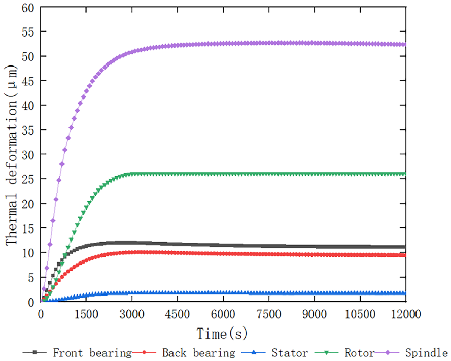
Thermal deformation of parts of the motorized spindle.
As shown in Figures 12 and 13, the longest time is needed for the spindle to reach an equilibrium of thermal deformation, which is mainly due to its large volume and significant thermal capacity.
Response surface analysis based on the steady-state thermal model
When the finite element model is used to predict the thermal deformation of the motorized spindle, it is necessary to recalculate the boundary conditions for simulation every time under changing working conditions. Consequently, to predict the thermal deformation quickly and comprehensively, the response surface model based on the finite element model is established in the present work. Meanwhile, the response surface model is used to optimize the parameters of various factors affecting the spindle thermal deformation, which provides a basis for the control of thermal deformation. The response surface method uses an explicit response surface to approximately solve the complex implicit relationship between the objective function and the n-dimensional vector by constructing a polynomial of the objective response function y and the n-dimensional vector
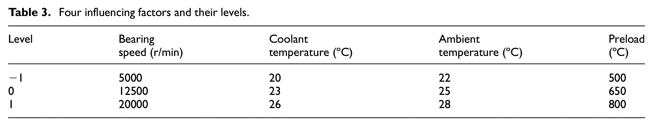
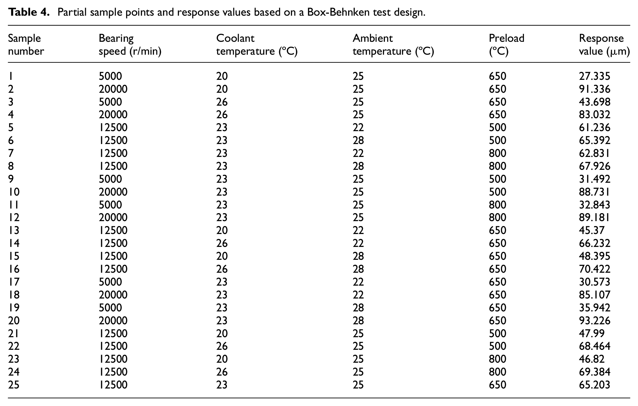
Considering the number of sample points, the feasibility of the experiment and the fitting accuracy of the response surface, Box-Behnken experimental design is used to select reasonable samples in this paper, and the major influencing factors and their levels are listed in Table 3. The response values of the sample points are obtained by the simulation experiment based on the steady-state thermal model, as listed in Table 4.
Four influencing factors and their levels.
Partial sample points and response values based on a Box-Behnken test design.
Design Expert response surface analysis software is used to establish the response surface model of the steady-state thermal elongation of the spindle under the interactions of various factors (Figure 14). Point A represents the prediction using the response surface model of 43 μm when the bearing speed is 12,000 rpm and the coolant temperature is 20°C. Point B denotes the prediction using the response surface model of 65 μm when the bearing speed is 12,000 rpm at a coolant temperature of 26°C.
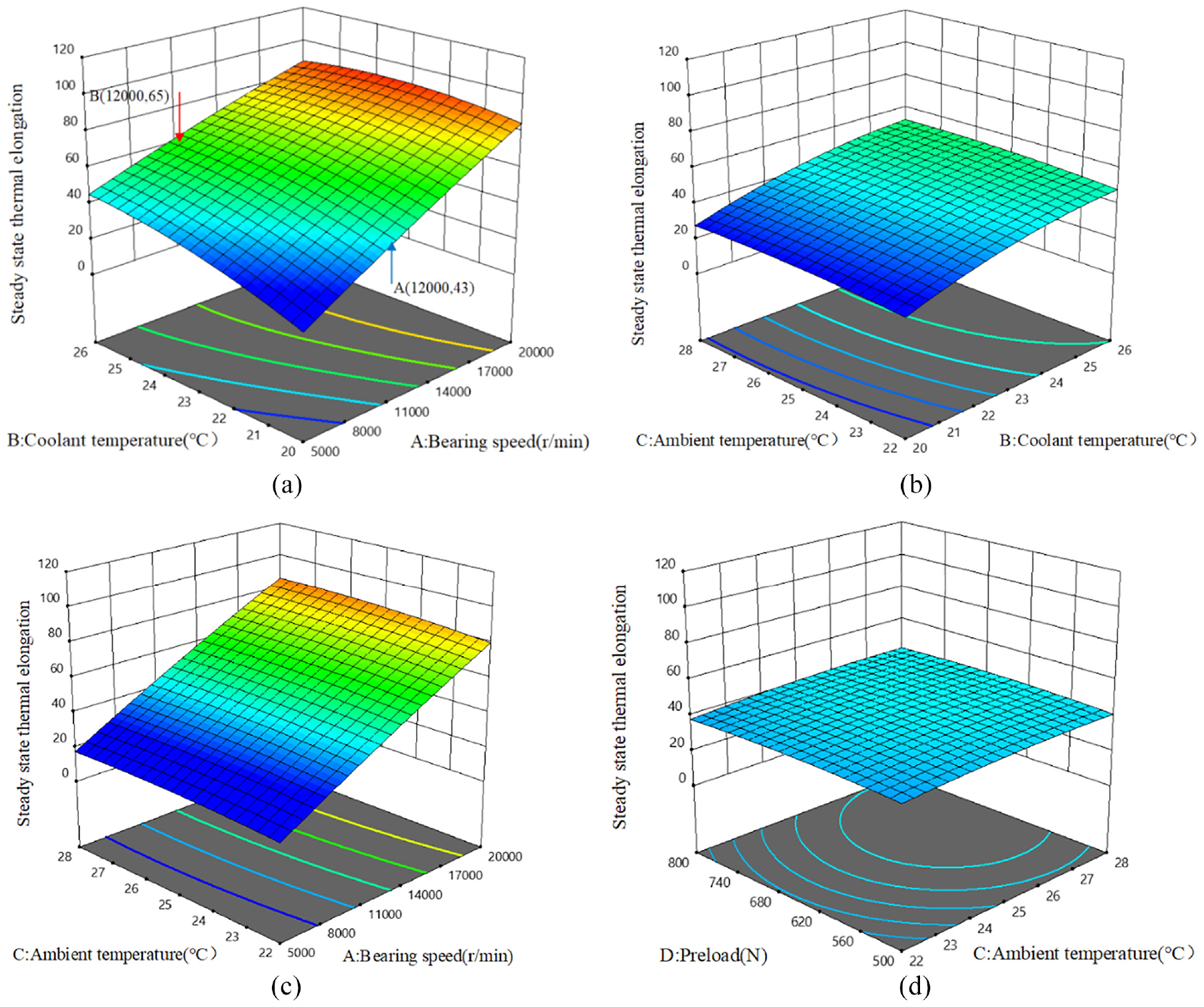
Response surface model of the interaction between factors and steady-state thermal elongation of the spindle: (a) the response surface of factor AB, (b) the response surface of factor BC, (c) the response surface of factor AC, and (d) the response surface of factor CD.
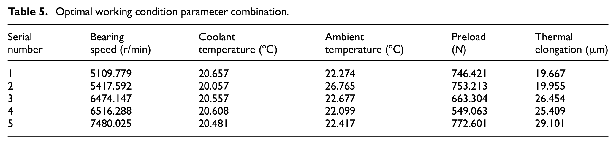
After the response surface model is established, specific influence rules of the parameter changes of each factor on the spindle thermal deformation can be revealed. In addition, the thermal elongation can be controlled through the optimal combination of each factor level. As shown in Table 5, when the steady-state thermal elongation of the spindle is controlled within 30 μm, the optimal combination of each factor level is obtained, which provides data in support of the regulation of the temperature and thermal elongation of the spindle.
Optimal working condition parameter combination.
Experimental verification
To verify the accuracy of the finite element model and the response surface model based on the heat flux application method compared with the traditional method, an experimental platform for measurement of the thermal characteristics of the motorized spindle is established. In the experimental measurement of the thermal properties of the motorized spindle, the hardware of the temperature measurement system is mainly composed of a temperature round measuring instrument, DS18B20 temperature sensors, a RS485 communication interface, and a UT-890K transformation module. As for software, the secondary development based on the fast-control configuration software is adopted. For the specific arrangement of temperature sensors, measurement points are arranged as shown in Figure 15 according to research results in previous research.25,26 Furthermore, to better measure the temperature of the motorized spindle, thermal conductive silicone is adopted to fill the air gap between the sensors and the contact surface to enhance the thermal conduction. According to the cloud pictures for the transient thermal deformation in Figure 10, the thermal error at the motorized spindle is mainly concentrated in the axial direction. Therefore, the axial thermal error at the end of the spindle is measured (Figure 16).
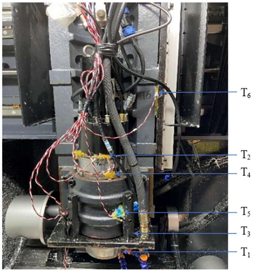
Experimental set-up of the temperature sensors.
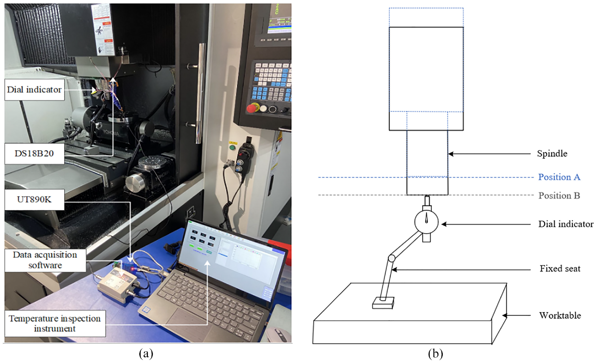
(a) Thermal error experimental measurement site and (b) schematic diagram of experimental measurement of thermal deformation.
The experimental object is the motorized spindle of TC-E650 CNC machine tool. The motorized spindle is set vertically in the machine tool and can be used for milling. When the experiment starts, the mechanical coordinates of the machine tool when the dial indicator is zeroed are taken as the reference coordinates and then the G-code of the motorized spindle is controlled to let the motorized spindle to move upwards by 5 mm along the positive direction of the Z-axis. At this time the front face of the motorized spindle is arrived at the position A, and kept at a safe distance from the probe of the dial indicator. Then the motorized spindle is allowed to rotate for 10 min at the position A. After the rotation is stopped, the motorized spindle is moved downwards by 5 mm along the negative direction of the Z-axis to the origin of the reference coordinates and arrived at position B. After allowing the motorized spindle to remain still for 10 s, the reading on the dial indicator is recorded, which is taken as the thermal displacement of the machine tool after operating for 10 min. Thereafter, the program is used to control the motorized spindle as it is shifted upwards by 5 mm along the positive direction of the Z-axis again to repeat the above process until the measurements of thermal deformation remain stable. That is to say, when the motorized spindle rotates at the position A for a period of time
To compare the specific differences in the prediction results of the thermal deformation of the motorized spindle between the two load application methods, the motorized spindle is tested at a constant speed of 10,000 rpm. The temperature measured in the experiment is shown in Figure 17. The comparison between experimental and simulation results indicates the following conclusions:
The temperature of each motorized spindle component will fluctuate, the temperature fluctuations at measurement points are caused by two factors: one is that the temperature of coolant liquids outflowing from the cooling machine changes periodically around the pre-set temperature of the cooling machine; the other is that the coolant liquids constantly absorb heat while flowing through the spiral cooling pipes, which results in a rising temperature and gradually weakened convective heat transfer capacity. Under joint action of these two factors, the coolant liquids do not have a constant convective heat transfer coefficient and therefore their cooling effect on the stators also varies, thus influencing the overall temperature distribution of the motorized spindle. However, the convective heat transfer coefficient of coolant oil is assumed to be constant for the convenience in finite element analysis.
On the whole, the temperature at measurement points rises significantly within 2000 s, then increases slowly, and tends to stabilize at about 3000 s, the simulated results are similar to the experimental results.
Specifically, the highest temperature of the front bearing is about 37°C, and the lowest temperature of the stator is about 28°C, and the temperature of other parts in order from high to low is the main spindle, rotor and back bearing.
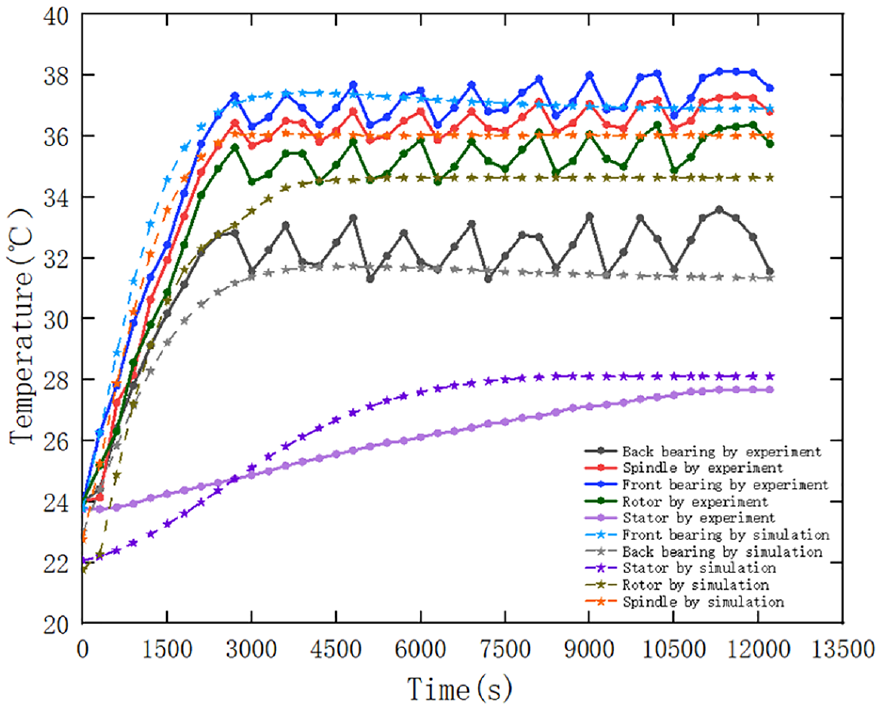
The comparison between experimental and simulation temperatures.
The comparison between the thermal deformation obtained from the experiment and the simulation results of the two load application methods is shown in Figure 18. The simulation curve of the prediction model applying loads based on heat flux indicates that the thermal deformation of the spindle reaches a steady state after 4500 s, both the value and trend are in good agreement with the experimental curves: the simulated value of the spindle final elongation is 52.31 μm, the experimental value is 48.5 μm. While the simulation curve of the prediction model applying loads based on the rate of heat generation shows that the thermal deformation of the spindle reaches a steady state at 3000 s, some 1500 s before that measured in this experiment. The simulated value of the spindle final elongation is 39.53 μm, having a larger difference as compared with experimental results. Therefore, compared with the traditional model, the finite element model applying loads based on heat flux has better predictive ability.
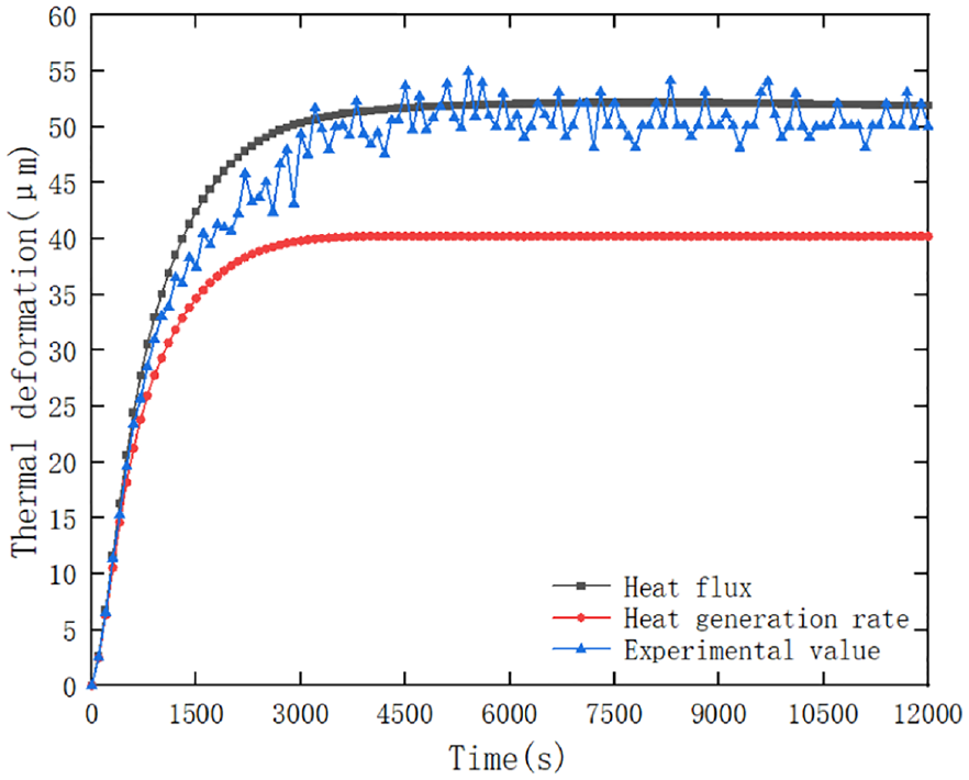
Thermal deformation of a motorized spindle.
In addition, it can be seen from Figures 17 and 18 that, both temperature and thermal deformation, the results of simulation analysis always increase gradually, while the results of experimental measurement also increase gradually on the whole, but there are fluctuations in a local scope. The main reason for this error is that, on the one hand, vibration caused by high-speed spindle rotation has a certain impact on measuring equipment. On the other hand, in order to reduce the computer analysis time, the motorized spindle model is simplified, and some conditions are simplified in the calculation process of boundary conditions, which leads to the simulation analysis results cannot be completely consistent with the experimental results.
Finally, to verify the response surface prediction model of the thermal deformation of a motorized spindle, the variable working condition experiment is conducted at a running speed of 12,000 rpm. The temperature of coolant in the cooling machine is first set to 26°C. During the experiment, when the temperature is quasi-constant and reaches the thermal steady state, the temperature of the cooler is reset to 20°C to continue the experiment (the motorized spindle is run for 3600 s). The measured temperature and axial thermal deformation of the motorized spindle are shown in Figure 19. Two points A and B in Figure 19(b) represent the axial thermal deformation of the motorized spindle with two coolant temperatures at the same speed. The thermal deformation reaches the thermal equilibrium state for the first time at point A at about 4200 s, and the thermal deformation at that time is 61.8 μm. When the coolant temperature decreases, the thermal deformation of the spindle does not decrease immediately, rather, it begins to decrease some 600 s after the coolant temperature is changed, and the thermal equilibrium state is reached again at point B at about 8700 s (when the thermal deformation is 43.9 μm). The experimental results are basically the same as the prediction results of response surface model in Figure 14(a), indicating that the response surface model can predict the thermal deformation of the spindle. Since the response surface model is established based on the simulation data of the finite element model. The experimental results can also verify the robustness of the finite element model.
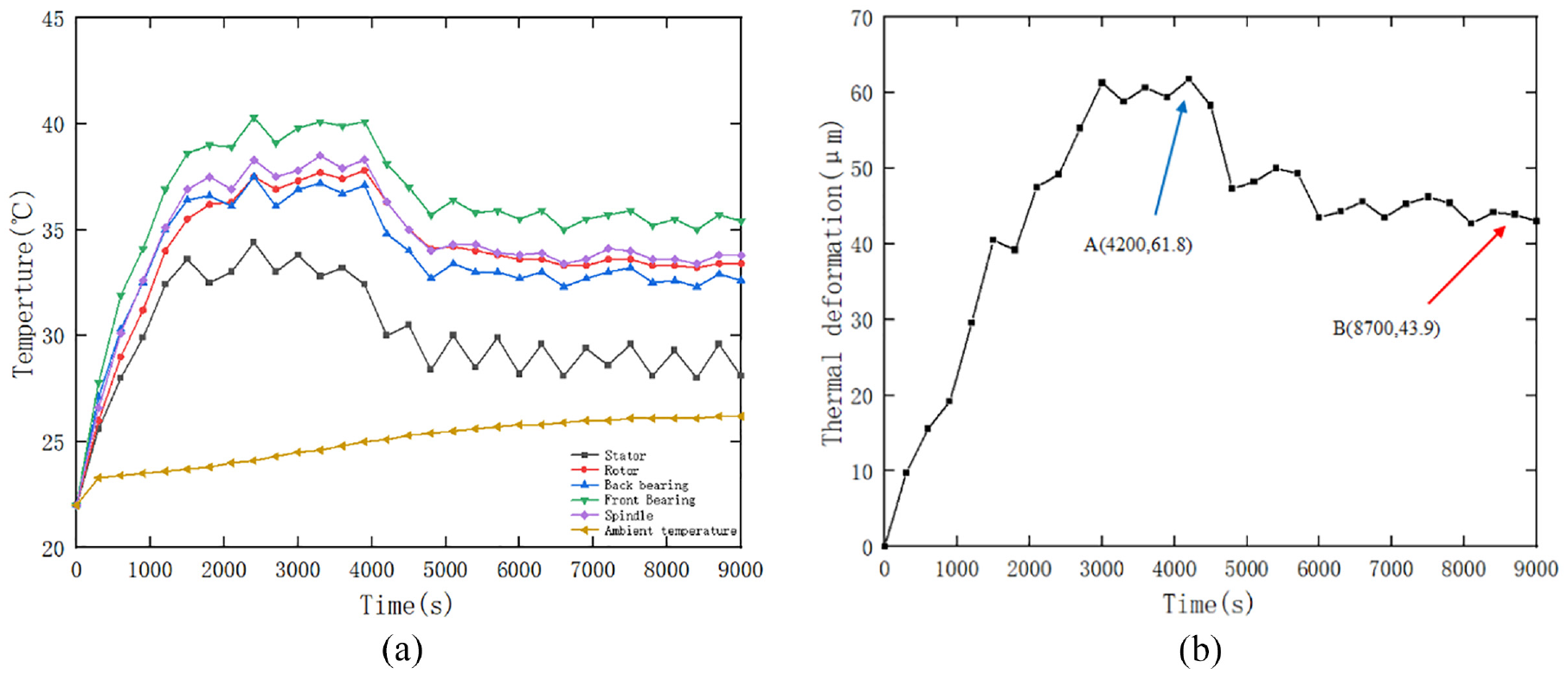
The measured temperatures and axial thermal deformations of a motorized spindle: (a) temperature measurements and (b) thermal deformation of a motorized spindle.
Conclusion
A modeling method of motorized spindle thermal errors by applying loads based on heat flux is proposed to improve the prediction accuracy of steady-state and transient thermal errors, and the effectiveness of the finite element model described in the method has been verified experimentally. The main conclusions are as follows:
The steady-state simulation accuracy under the loading mode based on heat flux is higher than that under the loading mode based on the rate of heat generation. The time to thermal equilibrium under the loading mode based on heat flux in the transient analysis is more realistic. Therefore, the thermal boundary conditions applied based on heat flux are more accurate than that applied based on the rate of heat generation.
The response surface model can efficiently predict the steady-state thermal deformation of the motorized spindle under variable working conditions, enhancing the prediction ability of the finite element model. It also reflects the thermal deformation rule of a motorized spindle under multiple interacting factors, and the temperature and thermal deformation of the motorized spindle can be regulated through the optimal combination of each influencing factor.
Both temperature and thermal deformation, the results of simulation analysis always increase gradually, while the results of experimental measurement also increase gradually on the whole, but there are fluctuations in a local scope.
The finite element predictions of the thermal errors of the motorized spindle under the loading mode based on heat flux differ from the traditional predictive model based on the rate of heat generation. The former, on the one hand, considers the heat distribution in the angular-contact ball bearing sets to the front and rear of the motorized spindle; on the other hand, it considers the applicability of the load type in the thermal module in ANSYS Workbench to the actual load, therefore, the finite element predictive model for the thermal errors under the loading mode based on heat flux can improve the prediction accuracy achieved.
Footnotes
Appendix
Author’s contribution
Wang Haoshuo: methodology, software, writing (original draft preparation), experiment, and data processing; Chen Guangsheng: conceptualization, methodology, writing (review & editing), supervision; Sun Yushan: format checking, modification of figures and text.
Declaration of conflicting interests
The author(s) declared no potential conflicts of interest with respect to the research, authorship, and/or publication of this article.
Funding
The author(s) received no financial support for the research, authorship, and/or publication of this article.
Ethical approval
Not applicable.
Consent to participate
Not applicable.
Consent to publish
All co-authors consent to the publication of this work.
Availability of data
Data will be available upon reasonable request.