Sage Journals: Discover world-class research

Abstract

Machine Learning (ML) has proved to be successful at identifying and representing underlying relationships in large data sets which would be difficult to process manually. However, the large amounts of data required for unsupervised learning mean that these traditional approaches encounter problems where data is sparse. In addition, these models are often used with insufficient regard for the details of the underlying optimization process. This poses a problem in engineering where the ability to explain model predictions (explainability) is often a prerequisite. There is a particular issue where ML methods may reach a conclusion which does not agree with existing physical understanding. Further, for problems where some of the underlying physics is already known, the traditional ML approach is effectively using large data sets to “re-learn” existing physical understanding. A potential solution to these issues is the incorporation of physical domain knowledge into the model or its training process to produce Informed Machine Learning. This paper provides an overview of the current state of informed machine learning for application in engineering. Firstly, the definition of explainable machine learning is explored. A selection of methods that incorporate physical priories into the machine learning pipeline is then described, leading to a review of current applications of informed machine learning in engineering. As a result of this analysis, a taxonomy is developed which provides a potential path for method development.

Keywords

Informed machine learning transparency interpretability explainability review

Introduction

Machine learning (ML) has received significant research attention over recent years and with the introduction of neural networks (NNs) these algorithms have become commonplace in a variety of applications. This is largely due to their success at producing accurate and actionable insights from large data sets, difficult or impossible to do by human processing. However, traditional ML models often lack a clear explanation of the process and reasoning behind their decisions. As a result, the term “black-box” is often used to describe such algorithms, highlighting the lack of underlying understanding for why a particular decision has been made. This issue is particularly important for use of these algorithms in engineering and the physical sciences – where decisions frequently need to be explained and justified. Hence “explainability” is frequently necessary to ensure a physically acceptable value of the outcome, in which a high degree of confidence can be placed. Hence, as Brunton and Kutz suggest, “Data science is not replacing mathematical physics and engineering, but is instead augmenting it for the 21st century, resulting in more of a renaissance than a revolution.”¹ The key to achieving this physical consistency in ML model outcomes is a sustained exploration into the continuum between black-box machine learning algorithms and traditional mechanistic engineering models. Such research aims to create a new class of ML “gray-box” algorithms which combine the comparative computational efficiency of ML and its applicability to large or difficult problems with the generalizability of traditional mechanistic models. For the purpose of this review the term informed ML will be used to describe such models, though other terms such as “gray-box” ML or “physics-guided” ML are in frequent use.

It is important to note that the following survey is not an exhaustive review of the mathematical techniques and applications of informed machine learning for application in engineering. Rather, it aims to cover a broad selection of informed machine learning methods for a range of engineering outcomes. The paper is written from a mechanical engineering perspective and will include examples from fluid dynamics and solid mechanics. However, the reader will appreciate that the problems faced in different branches of engineering are often very similar, for example the solution of partial differential equations. Hence we hope that the review will be useful beyond the confines of traditional mechanical engineering. The rapid uptake of Neural Networks means that they are currently the most prominent application of ML in Engineering. This is a fast evolving and extremely diverse field and therefore published research can seem somewhat disjointed. This review aims to describe the main methodologies and propose a selection of opportunities for future development in a form which is accessible for practising engineers. Hence, the paper is structured as follows. Section 2 will further develop the definition of informed ML by defining transparency, interpretability and explainability. Section 3 will focus on the methods applied to develop informed-ML models. Section 4 highlights the current applications of these methods in order to assess their success at enforcing transparency, interpretability and explainability. Often the techniques can be used in conjunction with each other to create custom informed neural network architectures. For this reason these hybrid approaches are also described in addition to the main methods themselves.

Background

Terminology

Due to the relative infancy of informed ML, there is a lack of consistency among comparable literature when defining an explanation in the context of gray-box algorithms. Historically, this has raised a philosophical question of accountability.^2,3 In the context of engineering and the natural sciences there is arguably less ambiguity, as outcomes must be scientifically consistent with existing physical domain knowledge. However, questions still arise surrounding the extent to which a given informed-ML model can be explained. For the purpose of this review, methods will be assessed on their ability to incorporate specific techniques into the ML pipeline that create transparency and interpretability, giving rise to greater explainability and ultimately scientifically consistent, generalizable outcomes.

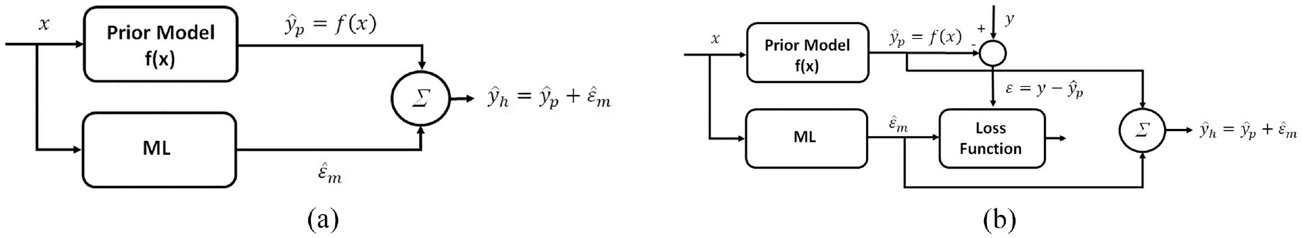
Generally, in engineering, incorporating domain knowledge into the ML model is achieved by enhancing input data, model architecture or the optimization process to reflect physical constraints such as algebraic and differential equations, probabilistic relations or simulation results.⁴ Roscher et al.⁵ view the process as shown in Figure 1, which provides a visual representation of the processes that lead to physical explainability. Firstly, the central box encompasses the process chain of a black-box ML algorithm in which the model is used as a method of producing an output from input data without any regard for understanding the optimization process. This may or may not produce a physically reasonable set of results. However, a more scientific outcome may be achieved by aiming to understand either the output results or the model itself. The figure introduces the two concepts which combine to give explainability: namely transparency of the model and interpretability of the results. As explained above, a traditional black box ML model is represented by the horizontal pathway through the middle of the diagram. Input data is used to train the model, which can then provide output for different sets of data. The model is not generalizable and it is impossible to understand the link between input and output data. Hence the term “black box.” In contrast, transparency is generally concerned with understanding the method of parameter extraction – the model itself. An example of this might involve hard coding a NN to incorporate the underlying physical relationship as a constraint on the output of every neuron. Hence, Daw et al.⁶ ensure that the output of a neuron is always physically consistent. In the particular case this requires a monotonic increase in water density with increasing depth. This means that there is a greater understanding of the optimization process as a direct result of incorporating physical insight. Thus, transparency is concerned with understanding the model itself, whereas interpretability is concerned with extracting meaning from the model in a manner comprehensible to a human. This is generally achieved through analysis of the model outcome. Hence, a model is interpretable if the output “makes sense” when viewed in the light of existing scientific knowledge. A combination of these principles of transparency and interpretability leads to the explainability of an informed ML model, whereby the incorporation of domain knowledge allows for an understanding of both the decision process and the output of the model.⁵ Hence, a model that is explainable requires both the model itself to be transparent and the results of running it on different datasets to be interpretable. Ultimately, using this approach should allow the development of models with increased physical consistency, applicable to domains beyond the training dataset.

Figure 1.

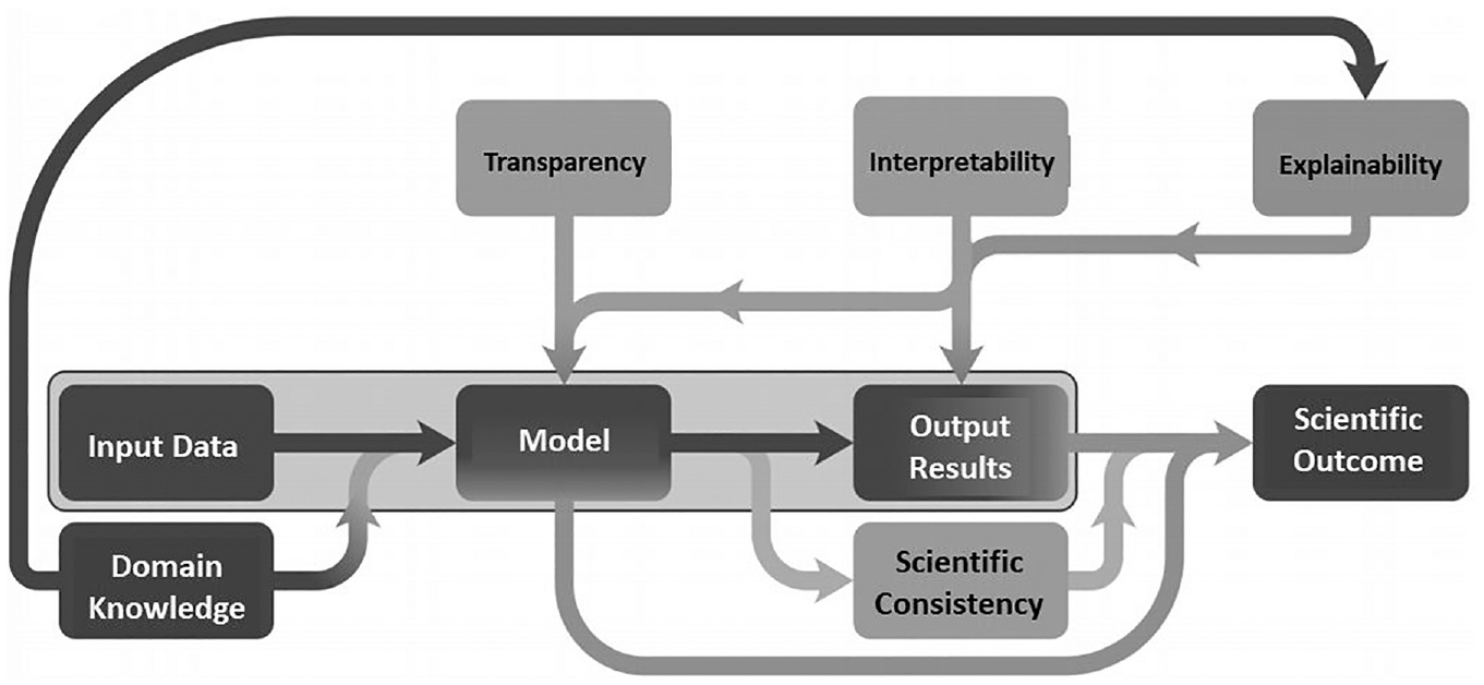
Schematic of gray-box ML pipelines for application in engineering.⁶

Historical Context

The idea of the Artificial Neural Network (ANN) was first introduced by McCulloch and Pitts.⁷ Here it was proposed that due to the “all-or-nothing” nature of biological nervous activity, a similar mathematical model could be produced based on propositional logic. This observation is used to build mathematical learning models that aim to mimic the human neural decision process by summing appropriately weighted neuron outputs. It is important to point out that the resulting network behavior is often described as a “neural network paradigm”⁸ and does not directly replicate that of a biological brain, since some of the limitations of traditional numerical mathematical techniques are transferred over.

Fundamental Principles of Neural Networks

Modeling the artificial neuron

Figure 2 depicts a pictorial representation of the neuron used in the development of ANNs. Essentially, each neuron receives a set of inputs $x_{i}$ , each of which are weighted according to weights $w_{i}$ . These are summed and combined with (if necessary) a neuron bias b. This can be represented by the equation $z = w^{T} x + b$ , where the weight terms w and inputs x are both vectors of equal dimension. The resulting value of z then forms the argument of a pre-set activation function, $Ø$ , which calculates the output of the neuron, y.⁹ Hence

y = ϕ (z) = ϕ (w^{T} x + b)

(1)

Figure 2.

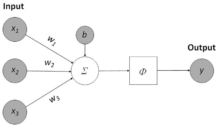
Block representation of an individual neural network neuron, after Emmert-Streib et al.⁹

Through a training process, the optimum value for each of the neuron weights is obtained in order to fit a given data set. This is achieved through repeated forward and backward passes of the network. Using Figure 2 as a reference, the forward pass moves left to right by taking the inputs to the neuron and summing them using equation (1). Conversely, a backward pass moves right to left on the figure. This involves comparing the resulting output to that of an expected output and implementing a gradient based optimization procedure (2.3.3) in which the input weights are altered in order to ensure the output is closer to that of the desired result. In a network involving a sequence of nodes this is often referred to as forward and backward propagation. Such a process corresponds to the artificial “learning” executed by a neural network whereby the model adapts these weights in response to the current output error.

Activation function

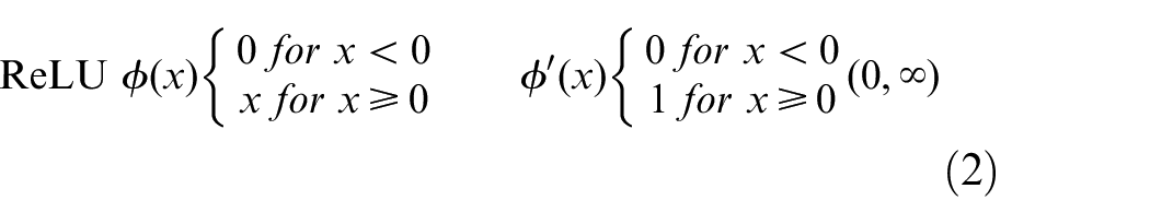
As explained above, once the linear weighted summation of the neuron inputs has been calculated to give the argument of equation (1), a non-linear activation function, $\emptyset$ , is applied to this summation value. One of the most popular functions for use in engineering applications, and indeed throughout the machine learning community, is the Rectified Linear Unit (ReLU). This is largely due to its simplicity which results in faster NN learning, as the output is equal to the input for inputs greater than zero and zero otherwise (equation (2)). This imposes the concept of a neuron threshold below which the neuron will have no influence on the following network interactions, much like its biological equivalent. Another advantage of ReLU is that for inputs greater than zero the gradient is non-zero during back propagation.¹⁰

ReLU ϕ (x) {\begin{matrix} 0 f o r x < 0 \\ x f o r x \geq 0 \end{matrix} ϕ' (x) {\begin{matrix} 0 f o r x < 0 \\ 1 f o r x \geq 0 \end{matrix} (0, \infty)

(2)

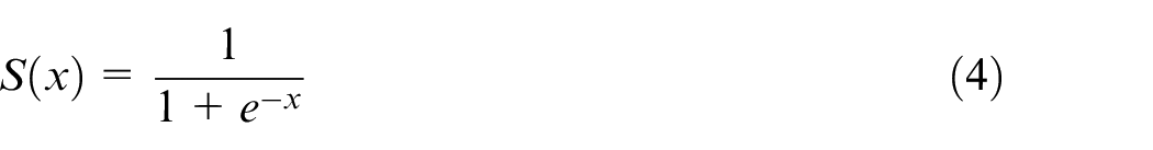
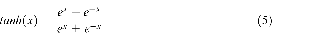
However, advancing research on physics-informed neural networks is helping identify areas in which the ReLU activation function is no longer optimum or applicable. Lagrangian Neural Networks (LNNs) have been designed to incorporate energy conservation equations. This is an example of an informed ML model as the network is constrained by known physical laws. This network makes use of the Hessian of the LNN – its second order derivative matrix. The second order derivative of the ReLU activation function is zero everywhere. Therefore, in this case it is not suitable and it must be replaced with a function of increased complexity that offers smooth differentiable output values. Cranmer et al.¹¹ used the Softplus function, given by equation (3) and shown in Figure 3(a). Other popular functions include sigmoid activation (equation (4), Figure 3(b)), which is advantageous as it outputs values between 0 and 1, as well as the Hyperbolic Tangent (tanh) which offers outputs ranging from −1 to 1 (equation (5), Figure 3(c)). Both of these allow for simple threshold implementation that can result in greater training performance.

Figure 3.

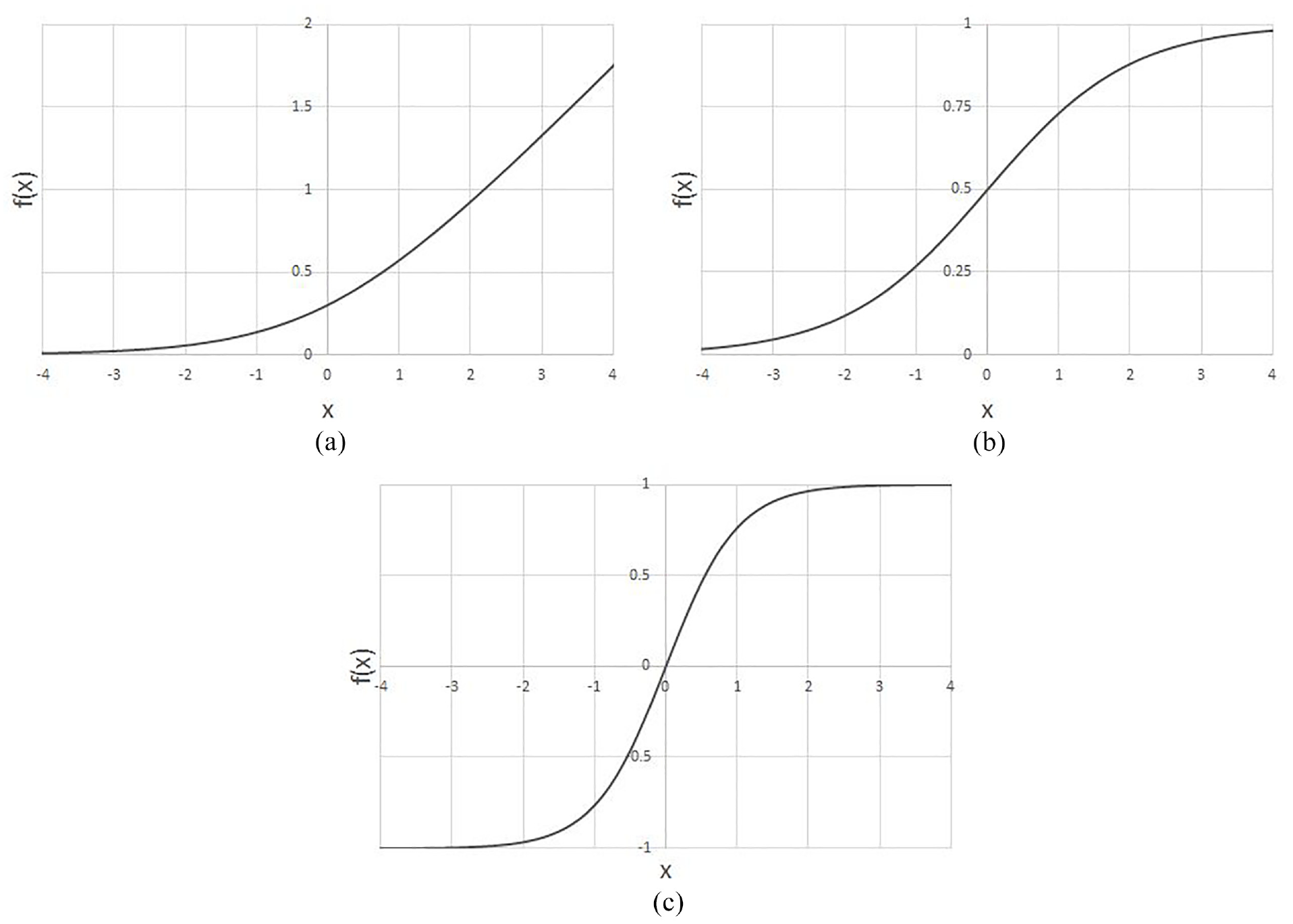
Different activation functions: (a) Softplus, (b) Sigmoid, and (c) Hyperbolic tangent.

Softplus

f (x) = \log (e^{x} + 1)

(3)

Sigmoid

S (x) = \frac{1}{1 + e^{- x}}

(4)

Hyperbolic Tangent

\tanh (x) = \frac{e^{x} - e^{- x}}{e^{x} + e^{- x}}

(5)

The final output of these activation functions forms the last layer of the neural network. In traditional NNs, where there may be as little as one output neuron, these values represent the probability of a given outcome for a particular set of input parameters. Examples of this type of output occur in solving for parameters in a partial differential equation¹² or identifying structural damage from an input image.¹³

Loss function

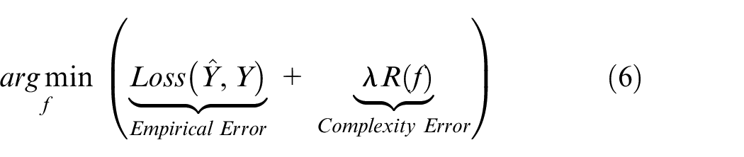
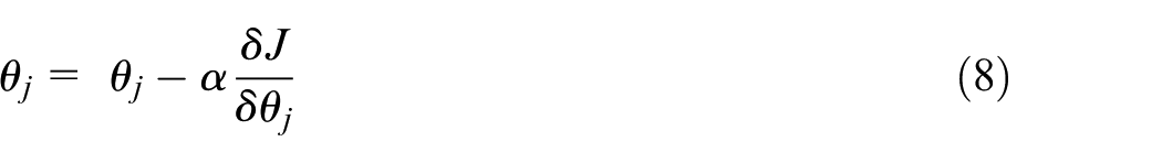
The loss function allows the NN to adapt at each iteration in order to “learn” the desired behavior. As mentioned earlier, this is commonly achieved in the training phase through backpropagation in which the network computes the current error between the desired algorithm output and uses this to update the weights at each neuron, moving backwards through the network. The most generalized form of this equation used in black box models can be seen in equation (6)¹⁴:

\underset{f}{\arg min} (\underset{Empirical Error}{\underset{︸}{Loss (\hat{Y}, Y)}} + \underset{Complexity Error}{\underset{︸}{λ R (f)}})

(6)

Here, $R (f)$ is a measure of the model complexity. This is often determined by the total number of features or terms – such as neurons and connections present – as well as factors such as the linearity of the functions that make up the model. Hence, the minimization attempts to strike a balance between minimizing the error between the model output and the training data and keeping the model relatively simple. It is desirable to minimize NN complexity for computational reasons and it will frequently have a clear minimum value for a given application and a prescribed output accuracy. In equation (6), $λ$ is a model hyper-parameter that controls the significance of the model complexity. The Loss function describing the model error with respect to the training data $Loss (\hat{Y}, Y)$ is often denoted as $J (θ)$ . The most common method of weight optimization, due to its simplicity in computational operation, is termed gradient descent in which the model parameters move toward a function minimum, guided by the steepest gradient of the loss function. As stated above, the goal is to minimize the error from the desired output using the current value which can be mathematically denoted by $(\hat{Y} - Y)$ . Therefore, taking m data points the total mean square error can be denoted as¹⁵:

J (θ) = \frac{1}{2 m} \sum_{i = 1}^{m} (\hat{Y} {(x)}_{i} - Y_{i})^{2}

(7)

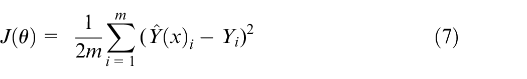
Finally, by taking the derivative of the loss function in equation (7) with respect to a given weight ( $θ_{j})$ , the weights are updated throughout to obtain a new set of “improved” weights as below:

θ_{j} = θ_{j} - α \frac{δ J}{δ θ_{j}}

(8)

In this equation $α$ is a constant learning rate chosen by the user. As is the case with the activation function, there are a variety of methods available for implementation of the loss function into machine learning models.

Neural network architecture

Figure 4 shows a fully connected feed-forward Deep Neural Network (DNN). Generally, the notion “deep” refers to NNs possessing more than one hidden intermediate layer. Each node in the figure denotes a programed neuron as previously introduced. These are the most widely implemented neural networks, both in black box modeling and informed machine learning, due to their theoretical simplicity and comparative ease of implementation. Their superior performance when dealing with non-linear, complex relationships also lends themselves to engineering domains.¹⁶ However, like many aspects of machine learning there are a variety of more task specific neural network architectures. Due to the relative infancy of informed machine learning in engineering, a coherent representation of the nature of this field does not exist. However, there are promising examples of Recurrent Neural Networks (RNNs) for thermodynamic temperature modeling of water,¹⁷ Convolutional Neural Networks (CNNs) in manufacturing,¹⁸ and Long Short-Term Memory NNs (LSTM) in chemical processing.¹⁹ A brief description of the architecture in question will be given as required throughout the remainder of the paper.

Figure 4.

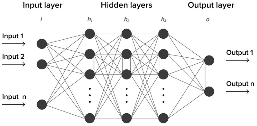
Schematic representation of a feedforward deep neural network, after House of Bots.²⁰

Physics informed ML methods

One of the most significant limitations of traditional black-box machine learning algorithms is their inability to generalize to situations outside the limits of the training data set.²¹ In addition, black-box methods clearly lack the ability to constrain the output to physically consistent values. In order for these algorithms to identify more generalized behavior, several new techniques have been developed to create outputs of greater physical consistency, resulting in greater extrapolability. Current research effort on these techniques is vast and extremely varied. Therefore, this section aims to introduce a selection of the most promising methods for informed-ML modeling and cannot be exhaustive.

Physics informed loss function

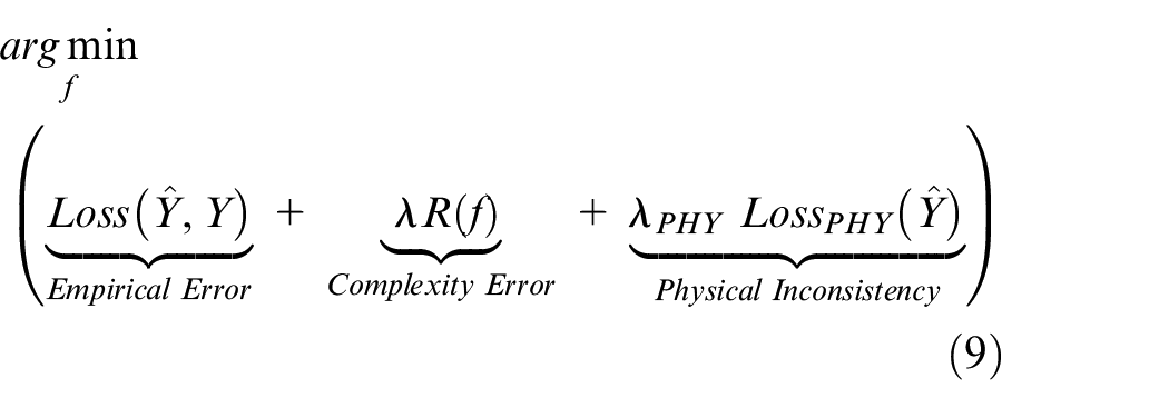
One of the most common methods of imposing physical consistency on the outcome of a machine learning model uses a physics informed loss function to penalize the model for predictions that violate physical laws. This adds a third term to the general equation (6), summarized in equation (9) below.

\begin{matrix} \underset{f}{\arg min} \\ (\underset{Empirical Error}{\underset{︸}{Loss (\hat{Y}, Y)}} + \underset{Complexity Error}{\underset{︸}{λ R (f)}} + \underset{Physical Inconsistency}{\underset{︸}{λ_{PHY} Los s_{PHY} (\hat{Y})}}) \end{matrix}

(9)

where $λ_{PHY}$ and $Los s_{PHY} (\hat{Y})$ represent the weighting of the physics-based loss function and the function itself. An illustrative but widely referenced example of this models lake temperature profiles using a hybrid Physics-Guided Neural Network (PGNN) depth.¹⁴ The model is influenced by an external mechanistic “General Lake Model” (GLM) in conjunction with a loss function that accounts for the monotonic increase in water density with decreasing depth.¹⁴ At a given time step this can be represented by the relation $ρ [d_{1}, t] - ρ [d_{2}, t] \leq 0, if d_{1} < d_{2}$ . If the density difference was calculated to be positive, its error was included using a non-zero instance of the ReLU function ( $ReLU (Δ ρ [d_{i}, t])$ ), these terms were then summed to find the mean of all physical violations across all depths and taken to be the physical inconsistency term in equation (9). In this instance, the model was tested against the baseline GLM as well as the hybrid model feeding a black-box NN algorithm. It was found that with the addition of the physical inconsistency loss term both the model root mean square error (RMSE) and the physical inconsistency were minimized. In contrast, the control hybrid model feeding a black box algorithm optimized RMSE but encountered physical inconsistencies as high as 73%. A continuation of this work used the same physical density constraint described but replaced the aforementioned hybrid model with a Physics Guided Recurrent Neural Network (PGRNN) that incorporated Long Short Term Memory (LSTM) cells. These cells allow for new processes to be included, such as forget gates that can act on stored information in order to control the gradient descent. In this example, the LSTM cells were used to constrain the learning process to physically consistent individual cell outputs by accounting for the underlying energy conservation equations in the form of changing heat flux.¹⁷ This work supported the significance of a physical constraint on the output of the model by also testing the effect of varying training data set size on the model performance. It was found that the PGRNN with physical constraint consistently produced lower errors (RMSE) than the standard RNN equivalent. It was also found that there was a significant reduction in physical inconsistency due to the inclusion of the physical loss term.

One of the most promising advantages of physics informed loss is the potential to introduce a simple method of unsupervised learning. Unlike the general loss function applied in black box models which requires large, labeled data sets to “compare” to the predicted outputs, physics informed loss terms are calculated based on pre-programed fixed relationships. This means that no further input is required following initialization. In contrast, traditionally black-box algorithms frequently require corrective human input. This is particularly important for engineering application where there may be a lack of real world data or where mechanistic simulations used to produce physically consistent data sets are too computationally expensive. The examples for lake temperature profiling above both make use of all three terms in equation (9), however if one could implement an informed-ML model without including the empirical error term, unsupervised learning could be realized. Once trained in this way, the network could be used to predict other sets of inputs and hence obviate the need to use a potentially complex mechanistic model for every case required. This concept has been explored for use in computer vision problems used to track objects in freefall.²² In this case, the parabolic height relation was used along with a fixed gravitational acceleration to penalize the model outputs during learning. This showed that although the unsupervised network resulted in a 90.1% correlation, compared to 94.5% correlation achieved for an equivalent supervised control algorithm, there is potential for a NN to extract physically consistent predictions by incorporating only the equations of physics that must be obeyed.

An interesting recent application in solid mechanics has been provided by Haghihat et al.²³ They have developed an approach which incorporates the equilibrium and compatibility equations of solid mechanics into the loss function. Their approach makes use of graph-based implementation of feed-forward network (see, e.g. Tensorflow²⁴) to provide accurate differentiation of stress and displacement variables. It was demonstrated that incorporation of the underlying physical equations in this way significantly reduced the training requirements. A similar approach was adopted by Abueidda, Lu and Koric,²⁵ who solved three-dimensional solid mechanics problems by incorporating the governing partial differential equations in the loss function.

Many applications of science and engineering involve multifaceted and correlated physical constraints. This is an aspect that the previous examples have failed to consider, but it is addressed in a study on the minimization of competing loss functions for general problems that can be represented by eigenvalue equations,²⁶ as commonly occurs in many fields of engineering. A key consideration, shown in Figure 5, is that in situations governed by these relationships there is an increased likelihood of optimizing to a local minimum due to competing conditions each requiring minimization. This example proposes a method for “adaptively tuning” the contribution of competing loss functions during training in order to produce generalizable solutions for two specific cases of the type mentioned above. However, the paper does not present an extensive theoretical approach that could be applied to other domains and applications in the future.

Figure 5.

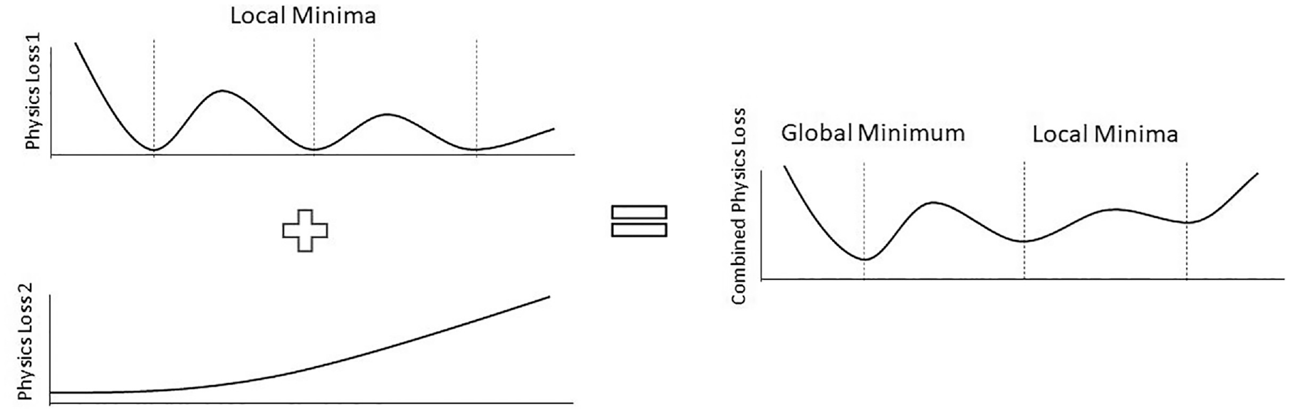
Visual representation of two competing loss terms which together have a global minimum.²³

Physics informed initialization

Physics based mechanistic models can be used to “inform” the starting parameters of a neural network before training. This is perhaps the simplest of methods for creating NNs with increased physical consistency. However, it is unlikely that this approach will be successful in isolation, as it does not guarantee physically consistent behavior but simply sets the starting conditions to a position that increases the likelihood of optimization to a global minimum. This means that physics informed initialization has the potential to combat the intrinsic susceptibility of ANNs to optimize to local minima, saddle points and flat regions. If these are reached they can often be indistinguishable from the target minima.²⁷ This approach would therefore be advantageous for the majority of ANNs applied in engineering. However, this method has also proved successful in applications where the available mechanistic models can produce coarse representations of the underlying physics with relative ease but require computationally expensive solutions at a fine temporal and spatial scale to capture the exact nature of the problem. This situation is particularly prominent in fluid dynamics simulations where the governing partial differential equations such as Navier Stokes can produce results for simple irrotational laminar flow but require methods such as direct numerical simulations (DNS) for more complex conditions. A key example is turbulence modeling, where there is a lack of available analytical solutions.²⁸ These flow solutions modeled in the physical domain lack the generalizability desired from informed-ML models due to the reliance on the specific flow geometry for calibration of the parameters. Alternatively, modeling the mean flow properties based upon the Reynolds Averaged Navier Stokes (RANS) equations, a set of partial differential equations decomposed to include both steady state and dynamic flow terms, allows for the prediction of a variety of different flow geometries.²⁹ A further example is provided by Mills et al. in the field of atomic physics.³⁰ They investigated the prediction of the ground state energy of an electron and noted that the electrostatic potential defined on a finite grid may be rotated in integer multiples of 90°. The convolutional neural network used does not capture this symmetry automatically, so they chose to train the network on an augmented data set, which included the original together with rotated copies. In contrast, in the field of quantum chemistry, Wang et al.³¹ have employed deep neural networks for predicting the time variation of a control electric field, E(t), which enables a particular desired electronic transition. Here, they note that the transition probability is not very sensitive to the phase of E(t). Hence, the neural network may experience difficulty in learning the role of the phase. To overcome this, they used a cross-correlation approach to shift the predicted control field by a series of different phase values. In essence this represents a physics informed interpretation and modification of the predictions of the network. These examples highlight the potential of physics informed initialization or physics informed interpretation for helping bridge the gap between mechanistic models and black-box algorithms.

Physics informed architecture

Many informed-ML techniques are primarily concerned with creating algorithms of increased interpretability. However, physics informed architecture has the potential to implicitly encode model transparency for application in the physical domain. This has the potential to equip engineers and scientists with the ability to identify new causal relationships which is likely to be a key advantage of future applications of informed-ML. As expected, potential options for implementing this approach are diverse and can often be extremely task specific. However, there are a number of options relevant to engineering applications which recur in the literature. These are discussed below.

Intermediate physical variables

The incorporation of intermediate physical variables has been explored through the further application of lake temperature modeling introduced in Section 3.1. Similarly to Jia et al.,¹⁷ an RNN – LSTM neural network architecture was chosen. However, here it was used to allow for the density $Z_{d - 1}$ at the previous depth to influence the following predicted density $Z_{d}$ by “preserving” the previous value within the model architecture.⁶ This is represented in Figure 6 by the workflow highlighted in red which implements ReLU activation to ensure that the change in density $δ_{d}$ remains positive. This application uses the same monotonic density-depth relation as in Karpatne et al.,¹⁴ however in this case it is directly hard coded into the architecture so that it can influence the forward pass prediction phase. This is different from the previous example which only utilized this relation to add to the total error of the entire model output. This method is particularly useful in cases where it is desired to apply uncertainty estimation procedures such as the Monte Carlo (MC) method which systematically “switches-off” random neurons throughout the network in order to produce an estimated uncertainty distribution³². A known disadvantage of applying MC to ML models which only use physics informed loss functions is the resulting increase in physical inconsistency. Daw et al.⁶ by comparing the baseline physics informed loss LSTM network to the black-box LSTM as there was found to be no reduction in RMS error or physical inconsistency of the output between these methods. This is due to the neuron dropout introducing sufficient randomness to the NN weights to effectively “unlearn” the physical constraints. This highlights a prominent disadvantage when relying solely on physics-guided loss for increasingly complex NN engineering applications as this method does not influence the intermediary states of the neurons in real-time during forward propagation of the NN. As suggested, this can be combatted by implementing informed-NNs that incorporate intermediate physical constraints that ensure the physical consistency of the output. This was found to produce physical inconsistencies that approached 0% while also allowing for the analysis of uncertainty distributions.⁶ This technique has the potential to be applied to a variety of engineering domains. However, further task specific activation functions must be researched in order to be able to apply increasingly complex physical constraints on the intermediate values, as this example is rather limited due to the simplicity in the density-depth relationship.

Figure 6.

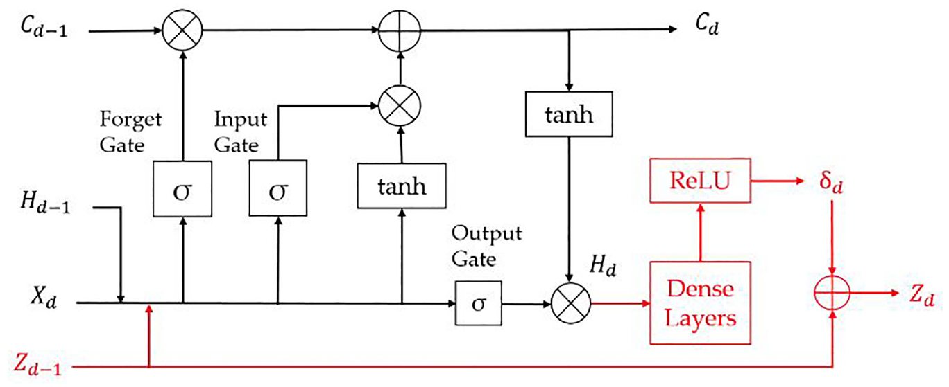
Schematic of model architecture incorporating intermediate physical variables represented in red.¹

This approach has been explored for an application of drag force prediction of particles.³³ In this case, Exponential Linear Activation (ELU) functions were incorporated within the network architecture to determine the pressure and velocity fields which can be utilized to impose physical constraints on the preceding predictions. This application was found to greatly outperform traditional baseline models in situations of data paucity. The method also allows for the comparison of intermediate neuron outputs to known physical theory, resulting in a model architecture that can be interpreted by experts in the domain.

Encoding invariances, symmetries and domain specific knowledge

Many aspects of engineering are determined by fundamental physical relationships that can be categorized depending on how the process changes as a result of a given transformation. This can be applied to the architecture of NNs to account for these mathematical invariances and symmetries. An illustrative example can be seen in the resemblance between translational symmetry and the conservation of momentum within a system.²¹ Due to their architecture, RNNs – in which the current output of a neuron is influenced by its previous output – would be expected to be able to account for time invariance relations. However, there is currently a lack of exemplary work using this technique. In contrast CNNs have proven most effective at encoding spatial relations due their ability at recognizing geometric properties, which make them extremely effective in applications such as image recognition. CNNs make use of convolutional kernels and are frequently used in image recognition. For example, a small group of RGB image pixels may be compared for similarity to the input in question. If the input is seen to have a high similarity – such as a value close to 1 on a 0–1 scale – then that selection of pixels is marked as identified in the image. In a standard case of image recognition, if a known selection of these kernels is identified together, the input image can be mapped to a known output image. Influencing the architecture so that more complex spatial invariances and symmetries are conserved has been explored for the case of translation, rotation, uniform motion and scale relationships. An example of this, developed an informed CNN architecture that provides informed-ML solutions to PDEs.³⁴ If an equivariant function input is transformed by a mathematically symmetric function g its outputs will transform equivalently:

f (g \cdot x) = g \cdot f (x)

(10)

In this case, the Navier Stokes (NS) equations were tested due the established equivariant nature of fluid flow. There is, however, uncertainty over how to normalize fluid flow data in order to share the same frame of reference. The predominant advantage thought to come from incorporating such behavior is the resulting generalizability of the model. These properties can be incorporated to ensure that the model output is equivariant to transformations of the input. As a result, the model would be applicable to domains not included in the training data set. This advantage was highlighted when comparing this method to its non-equivariant counterpart as the model proved to considerably reduce the Energy Spectrum Error (ESE) when tested on transformed – out of sample – data sets. ESE is a metric that can be used to identify whether energy conservation of a given system has been obeyed, critical to the realization of truly physically consistent ML models. This finding highlights the potential for incorporating domain knowledge of this kind into the ML pipeline in order to normalize fluid flow data for further generalized scenarios. Additional advances have seen similar results for chemical processing and will be discussed in Section 4.2.2.³⁵

Physics informed Gaussian process regression

Although, Gaussian Process Modeling (GPR) is not necessarily directly associated with physics informed architecture, it is a method that is thought to have potential to dramatically reduce a model’s data requirement. Therefore, in conjunction with the preceding methods it can prove to be a logical architectural design decision for engineering applications where this is often the case. GPR effectively measures the similarity between input points using a covariant kernel function. One instance utilizes the inclusion of the governing PDE into this function in order to incorporate physical insight. The output is not only associated with a predicted value but also a predicted uncertainty distribution.³⁶ This was applied to a variety of situations described by governing PDEs including the Burgers’ Equation – a simplification of the Navier Stokes equations which omit the pressure gradient term. This probabilistic approach proved to be applicable across each of these generalizable equations however it remained adversely affected by input noise and reduced training data. The advantage of this work over previous studies was its ability to predict parameters without a combinatorially large search through all possible candidate coefficients.³⁷ This approach will be further explored in Sections 4.3.1 and 4.4.2 which are concerned with modeling PDEs and quantifying model uncertainty using informed-ML models respectively.

Hybrid modeling

Hybrid modeling is a general term applied to algorithms that combine a physics based mechanistic simulation with a machine learning model to produce an informed-ML. This coupling can take differing forms depending on the application. Although hybrid modeling in isolation does not ensure explainability of the ML model in use – it does aim to increase the physical consistency of the combined model outcome. This means that explainability may be implicitly imposed.

One method seen in Figure 7 involves the use of a feedforward NN to learn from the residuals between the actual measured values (y) and the mechanistic model outputs ( $\hat{y}$ ) rather than the final output of the NN. This means that the training process in Figure 6(a) aims to minimize the difference between the sum of the mechanistic model and NN output compared to the measured values. This way, once trained, the NN can account for the missing behavior lost in the error of the mechanistic model, as seen in Figure 6(b). In a particular case of thermal engineering, this was applied to predict the critical heat flux in a two-phase flow boiling system.¹⁶ This hybrid method was found to consistently outperform the standalone mechanistic model due to many simplified assumptions used to derive the numerical solution – such as circular flow geometry which proved insufficient for other generalized conditions such as a flat plate. Therefore, the NN was able to account for these insufficiencies. Further analysis using a variety of sensitivity procedures found that the hybrid models effectively optimized RMSE in each case while also identifying data with up to 100% accuracy (allowing for ±20% error) and 96% accuracy (for ±10% error). The data split used was 90% training. 10% test.

Figure 7.

Schematic of a residual hybrid model accounting for the missing physics of a prior mechanistic simulation.¹⁶

In contrast to the situation above, for applications in which the mechanistic model is significantly more accurate, hybrid residual modeling may prove to be unsuitable, as its predictions may be negatively affected by the presence of scattered noise or randomness in the input data. This could result in overfitting instead of identifying the undiscovered trends. In situations where this may be the case, it may prove more suitable to instead use the NN to approximate the unknown input parameters from a system and use this as input to the mechanistic model alongside any measurable values. This method has been applied to model a fed batch bioreactor in chemical processing to account for the unknown kinetics of the conversion of substrate to biomass.³⁸ The advantage of this method for engineering application is the reduced data requirement for training, as the NN is only used to approximate part of the process – the unmeasurable parameters. The previous findings were supported as the hybrid model was shown to generalize to situations beyond the training data set with greater accuracy than the mechanistic model itself. As suggested above, the hybrid model was also found to reject noisy input data, even in situations where there was limited training data. A similar approach is seen in the case of lake temperature modeling introduced in Section 3.1.¹⁴ However, in this case the mechanistic model was used to achieve physically consistent outputs which were then fed into a NN that incorporated informed loss functions. Again, the final output therefore accounted for the physics not included in the numerical model.

Incorporating informed ML in engineering

This section is concerned with identifying how the preceding methods of informed machine learning are used to achieve a given engineering objective. Each of the most common objectives identified will be further distinguished by the method’s ability to impose transparency, interpretability and explainability on the model and its outcome. Due to space constraints, this will be achieved in two subgroups. The first concerns the incorporation of outcome interpretability leading to a basic level of explainability and the second encompasses methods that incorporate model transparency. These often also include methods of interpretability and inevitably lead to greater explainability, ultimately increasing the degree to which the ML methods are “informed.”

Improving predictions beyond traditional models

Computational mechanistic simulations have provided engineers with the ability to model complex physics-based problems without the need for experiment. However, these models pose two significant problems. They are often extremely time consuming, due to their computational size, and the physical laws utilized are often approximations of observed physics due to an incomplete knowledge of the domain. This latter aspect may introduce expert bias in the form of preconceptions and misunderstandings of the domain. This second problem is exacerbated by the fact that mechanistic models often require input parameters which are determined using limited observed data. Hence there is a degree of uncertainty in the model outputs. Machine Learning models have shown promise in mitigating these problems as they can be used to autonomously extract complex relationships from large data sets with reasonable computational efficiency.²¹ However, ML can also introduce limitations similar to those of traditional numerical techniques. The potential for “false discoveries” due to the presence of local minima or the identification of non-stationary relationships amongst the variables means that the incorporation of traditional black-box machine learning algorithms in engineering has seen variable success. As a result, a novel combination of machine learning and physics-based knowledge is required to not only improve predictions beyond mechanistic models but also to minimize false discoveries.

The approach described above is often applicable in situations where there is a lack of expert knowledge but an adequate quantity of good quality data is available.³⁹ Another possibility is that the mechanistic simulations do not utilize the full extent of the domain knowledge.⁴⁰ Therefore, from the view of the mechanistic simulation there is a lack of expert knowledge when compared to the reality of the underlying physics. Sections 4.1.1 and 4.1.2 will address an example of each of the instances.

Outcome interpretability leading to increased explainability

As suggested above, the engineering domain in which these techniques have had the greatest impact is most likely in fluid dynamic turbulence simulations, used in a range of engineering applications from aerospace to nuclear energy. The lack of underlying governing equations and the vast quantity of relevant parameters have made it difficult to design model transparent informed-ML algorithms. However research using a posteriori tests has produced outcome interpretability which may lead to increasingly generalizable informed-ML models in this field. Continuing from the work of Wu et al.²⁹ introduced in Section 3.2, attempts have been made to improve the generalizability of mean flow simulation using RANS in order to extract meaningful outputs of interest such as drag, lift and surface friction derived from the mean velocity.³⁹ In this work the ML method uses an invariant basis vector approach⁴⁰ to enforce a physics-informed implicit treatment of the Reynolds Stresses. This approach could prove useful for other domains in which the underlying processes are described by a large set of tensors. Here, a propagation test with direct numerical simulation (DNS) Reynolds Stress was used to interpret the ML model output, showing that it could produce accurate predictions of mean velocity. Further, the model was tested on a case outside the training set and was found to successfully predict the mean flow. This provides promising evidence of increasingly generalizable informed-ML models for turbulent flow simulations.

Applications that allow for outcome interpretability and basic model transparency

Figure 8 shows the full analysis pipeline for a case of bearing fault defect diagnosis using a physics-informed CNN (PCNN).⁴¹ Traditionally, a selection of signal processing techniques such as SK analysis⁴² and envelope analysis⁴³ have been used to manually extract characteristic features from raw sensor data. These have then been fed into a black-box machine learning model in order to identify the health of the bearing. In contrast the PCNN incorporates the rotational speed and fault-characteristic frequencies within the physics-based convolution layer. These quantities are used as the inputs for constructing the convolutional filters. In this respect the ML model is informed by incorporating ML hybrid techniques, that is, using more established physical methods as inputs, as well as actively adapting the kernels in the CNN architecture to reflect the differences between the input signal and the known fault-characteristic signals. This ensures that the NN architecture is uncharacteristically transparent as it removes the reliance on model hyperparameters to generate the kernels used for convolution, instead replacing these with physical simulation results based on reference fault signals.

ϕ [k] = a_{0} \sum_{s = 0}^{n} [H (k - s / f_{0}) \cdot e^{- ξ (k - \frac{s}{f_{0}})}]

(11)

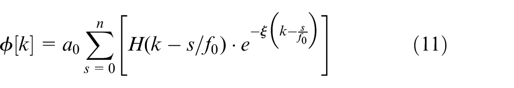
where k is the time index, a₀ is a constant amplitude that accounts for the radial load and fault severity, H(k) is the unit step function and simulates fault-induced impulses that switch on at time k = 0, f₀ is the fault-characteristic frequency of the defective bearing, and ξ is the damping coefficient. Implementation of the proposed method showed that the PCNN could both detect and localize faults with greater accuracy than traditional models. This is most likely due to the multi-channel convolution architecture which allows for the incorporation of multiple sensor inputs. The approach should be transferable to other instances of fault detection in the rotating machinery. A similar method for analysis of induction motor fault characteristics using physical insight in the form of time frequency spectra is presented by Grezmak et al.⁴⁴ In this instance however, transparent physics-informed kernels are not used they are replaced with a detailed analysis of the reliance of the output on input spectral frequency information. This means that the method is less transparent and more interpretable than the previous example. However it does offer a comprehensive review of the state of this field and supports the idea of transferability to a variety of other engineering domains.

Figure 8.

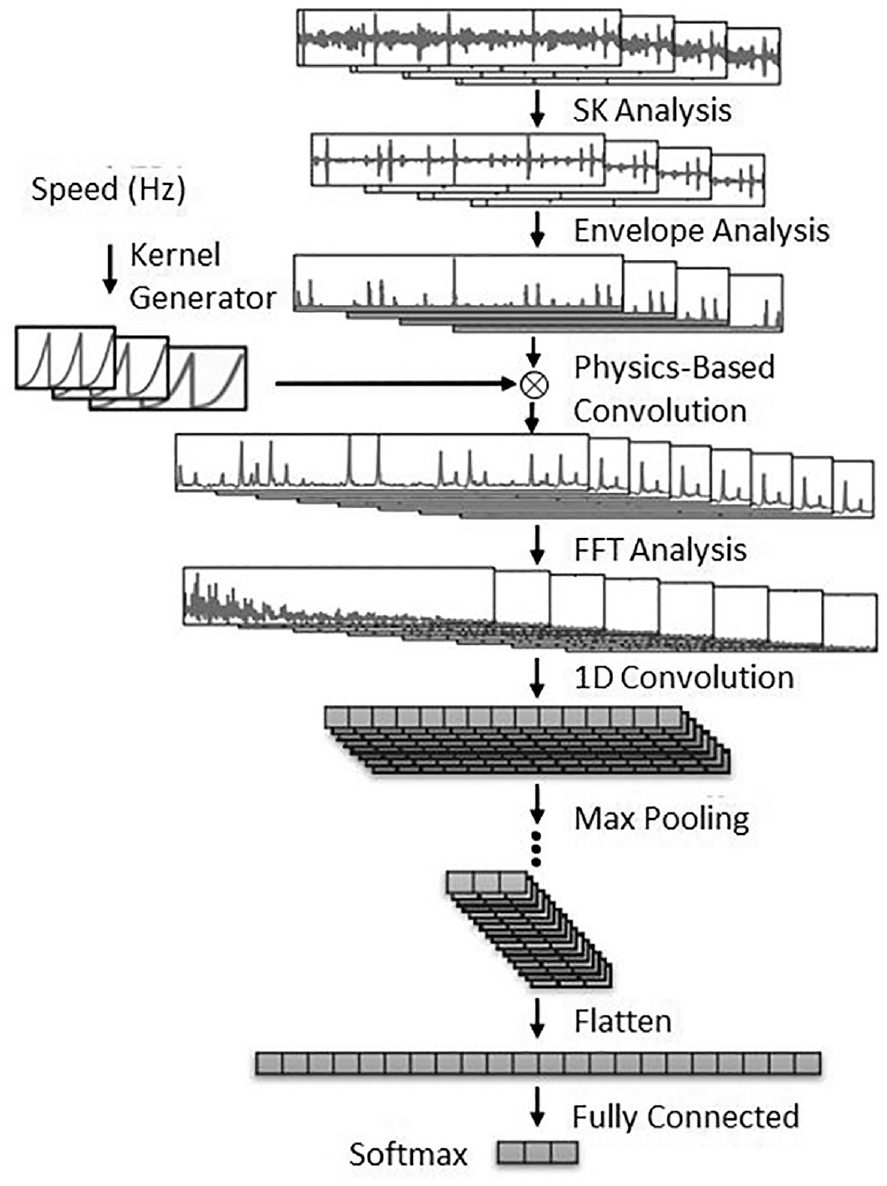
Physics informed-ML pipeline for a novel case of bearing fault detection.³⁵

Reducing Model Data Requirements

Mechanistic simulations run at a high resolution can capture physical behavior at a greater spatial and temporal scale than their lower resolution counterparts. However, this imposes greater computational cost, which often results in impractical times for complete simulation. As a result, many engineering simulations are run at a coarser resolution than is needed to capture the small-scale behavior of the physical system. In contrast, machine learning models provide the opportunity to incorporate several promising methods that mitigate these effects. These can be used either to imply higher precision behavior from input data, using methods such as downscaling and parameterization, or to process high precision input data such that the computation time is reduced by making use of Reduced Order Modeling (ROM) techniques which can be described as a “controlled loss of accuracy.”²¹

Outcome interpretability leading reduced model data requirements

Figure 9 shows the workflow for a hybrid model that incorporates ROM techniques for the prediction of mechanical stresses in a component due to manufacturing flaws.⁴⁵ In this case, simulation data is used to inform the clustering process performed by a CNN using a 2D image of the sample under loading conditions. Clusters are assigned to areas of similar mechanical loading based on known fundamental load-displacement stress relationships, before a set of hyper-reduced equations are solved as an inverse problem in order to identify the precise load location. This technique combats the spatial step limitations of numerical FEA stress simulations and is shown to be of satisfactory accuracy for the desired application for component-specific quality control. Its predominant advantage is the increase in computational speed which is particularly important for the intended application. The reason for the model only being considered as interpretable and not transparent, despite the seemingly explainable nature of the clustering process, is due to its heavy reliance on simulation data for parameter extraction. Therefore, the CNN itself is no more transparent than a traditional black-box algorithm. This also highlights another disadvantage of CROM for use in situations where the mechanistic simulation techniques fail to utilize the full extent of the available domain knowledge (as mentioned in Section 4.1).

Figure 9.

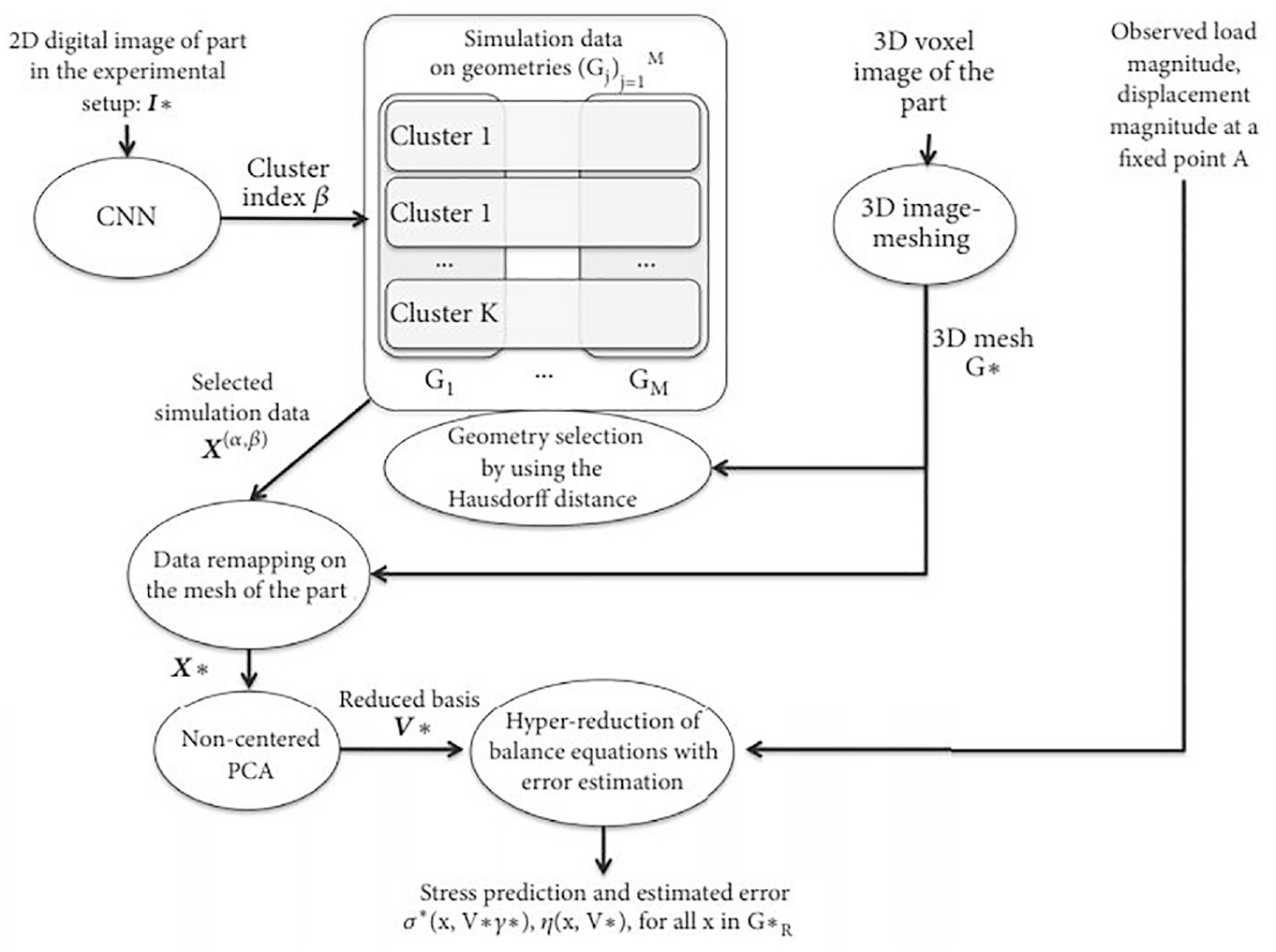
Schematic of the workflow for a convolutional reduced order model (CROM) used to identify stress concentrations in manufactured components – moving from top (inputs) to bottom (outputs).³⁸

This work was developed further both conceptually and mathematically in a study concerning an anisothermal elastoplastic application in structural mechanics.⁴⁶ Here a similar CROM non-parameterized, informed-ML method was used to predict structural damage due to a randomized temperature field. However, in this case a ROM dictionary of reduced complexity simulations was used to inform clustering. ROM dictionaries such as this define several lower order models based on distinct local subsets of the problem space. The study found that simulations utilizing the dictionary ROM clustering were executed up to 60 times faster than their non-simplified counterparts. This method therefore shows promise for application to increasingly complex situations by using greatly simplified FEA models as input. However, a clear disadvantage is that the CNN is influenced by a simplified version of the physical reality. This means that the model is less interpretable than the previous example since model clustering is more remote from mechanistic input, thereby reducing the model explainability.

Applications with model transparency leading to reduced model data requirements

Chemical engineering processing is another domain in which reducing model data requirements could prove critical in the development of informed-ML methods. Here, computationally demanding techniques such as density-functional theory (DFT) render mechanistic simulations unfeasible for extended processes. One example of this uses symmetries in atomic energy contributions to inform a NN and to produce physically consistent outputs.³⁵ Although an established data reduction method was not used in this instance, the primary concern was to reduce data requirements for accurate simulations. This example reflects the rapid nature in which informed ML is developing and that it allows scope to design new methods, more amenable to the inclusion of domain knowledge. In chemical processing the order in which the coordinates of atomic configurations are fed into the NN is not arbitrary as this can affect the predicted outputs. By using the physical symmetry relationships, a normalized method was produced which could be generalized to a range of situations. For this reason, this method is deemed to be transparent in comparison to the previous CROM methods as the NN processes the input information differently as a direct result of known governing physical principles. However, due to the continued reliance on model hyperparameters, the method cannot be said to be truly transparent as the reason behind the differences in optimization behavior due to these randomly selected values is still unknown. Rapid chemical process modeling, similar to the ROM methods above, has also been explored in order to develop a generalized method that can be applied to processes which are physically similar to the training simulation.⁴⁷ However, in this case the model does not attempt to incorporate interpretability or transparency into the ML pipeline. Instead it optimizes black-box model migration to generalized experimental processes.

Solving Engineering Problems

Partial Differential Equations (PDEs) are used throughout engineering and science to represent complex non-linear physical behavior. In many aspects of engineering, the exact governing equations are often not known. Alternatively, the mechanistic simulations used to represent these phenomena do not incorporate the full extent of the domain knowledge due to spatial and temporal computational expense. Both scenarios lead to a reduction in model precision. However, if the computational advantages of ML could be leveraged to mitigate this, while conserving physical consistency, then these informed-ML models would have the potential to both solve existing PDEs at greater step precision and to act as surrogate models for the solutions of new governing equations. The latter is made possible due to a NN’s ability to explore large domains of non-linear mathematical variables and is most likely achieved through inverse modeling, whereby the output is used to infer the intrinsic physical parameters.⁴⁸

Outcome interpretability used for solving problems in engineering

It is expected that the available techniques used for the discovery of new governing equations utilize little physical insight – beyond measurable quantities – due to the sparsity of domain knowledge in areas where such governing equations are a topic of research. It is also worth adding that many of these techniques are in their elementary mathematical stages, therefore applications are predominantly those that have been hypothetically tested by the authors of such work. One instance where this was found to be true was in a study that looked at the data-driven discovery of PDEs in parameterized spatiotemporal systems.³⁶ Here, it was desired to construct the relationship $N (\cdot)$ , from time series measurements of the system at fixed spatial locations x.

u_{t} = N (u, u_{x}, u_{xx}, \dots x, μ)

(12)

The Navier-Stokes equations were discovered through sparse regression methods used to determine the terms contributing to the behavior of the system. This was achieved without the requirement for a np-hard brute-force search across all term combinations. Remarkably, the method identified the underlying behavior within an accuracy of less than 1%. However, a fundamental disadvantage in this method for use in novel applications is that there is little way of analyzing whether the model has identified the correct governing equations. This results from the lack of transparency of the optimization process itself. This pioneering work has been developed further in Raissi⁴⁹ to reduce the spatio-temporal time series data requirements, thus reducing computation

Applications with model used for solving problems in engineering

The problem of governing equation discovery is addressed further in a paper that proposes a new informed-ML tool named PDE-NET 2.0.⁵⁰ This model uses numerical approximations of differential operators using a novel CNN architecture to discover time dependent PDEs from measured domain data. The key addition in this method is that there are constraints set on the kernels that increase the generalizability of the model to a range of domains and allow for longer time dynamics to be explored. In the context of this review, transparency is added to the parameter extraction process increasing explainability. These principles are illustrated in Figure 10, incorporating two hidden layers that are fed from the previous layer following a mathematical operation imposed by the kernel.

Figure 10.

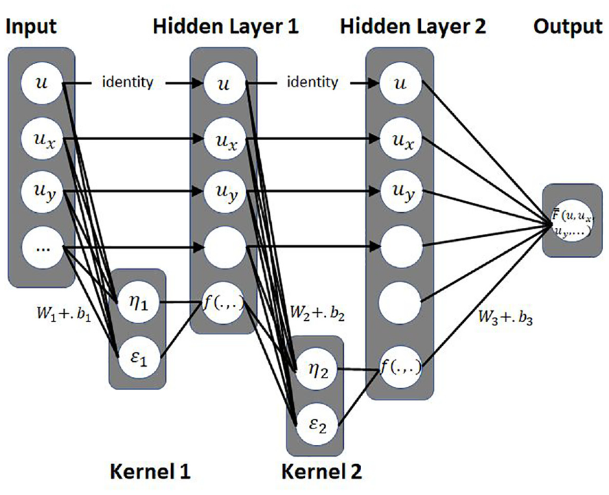
Schematic of informed kernels used in the convolution between network layers for the discovery of PDEs adapted from Meng and Karniadakis.⁴⁸

Significant research has tried to address the primary aspect of this section, concerned with solving PDEs in order to replace mechanistic models and leverage the computational power of ML. One approach proposed the development of Universal Differential Equations (UDEs) of the form in equation (13).⁵¹

u^{'} = f (u, t, U_{θ} (u, t))

(13)

Alongside, the arguments of the governing PDE, the UDE incorporates an embedded universal approximation in the form of a NN denoted by $U_{θ} (u, t)$ . This work allows for the simple combination of traditional mechanistic models with ML for a multitude of applications governed by PDEs of differing forms. This hybrid-approach means that physical consistency is conserved while ensuring efficient computation. Therefore, this is advantageous over exclusively numerical solutions and allows for the incorporation of domain knowledge in a variety of forms confirming the transparency of the method. In one instance this was utilized to incorporate conservation equations such as those used to describe a chemical combustion process. However, as this method is newly proposed and is the first of its kind, there is little knowledge on its real-world applicability in engineering. There are a variety of other approaches that have been proposed through literature, though none have shown the same level of transparency. One such novel approach has tried to mitigate the computational training requirement by utilizing low fidelity data in a multi-network structure.⁴⁸

Analysis of the resulting model outcomes

Finally, a thorough analysis of experimental and model outputs is critical in engineering, where design decisions often have safety implications. Traditionally this is referred to as uncertainty quantification (UQ). In order to uphold this principle, emerging informed-ML techniques for use in engineering must also be able to estimate model uncertainties. Essentially, this entails accurately characterizing the entire domain as the probability of y given x, $p (y | x)$ , where y is the output and x is a parameter input.²¹

Outcome interpretability used for analysis of informed-ML outputs

Basic level techniques that aim to quantify model uncertainty, incorporate interpretability in the form of a sensitivity analysis which identifies the contribution of each of the inputs to the model outcome. However, these techniques do not identify a comprehensive probability distribution of model outcome as described above. As introduced in Section 4.1.2, an example of this uses Layer-wise Relevance Propagation (LRP) at pixel-level precision to assess a signal’s contribution from an input image containing spectral frequency information on predictions of motor fault detection.⁴⁴ To summarize, this assesses the contribution of each neuron, backpropagated such that the total contribution in each layer is constant. Therefore, the sensitivity of each input pixel, corresponding to a neuron, can be compared proportionally to the others. There are a variety of task specific methods for calculating this neuron contribution, however in this case the “z-rule”⁵² was used. This was successful for this application as each of the fault signals tested were identified correctly, but it may not be applicable to real-world engineering use due to its sensitivity to input signal noise.

Applications that use model transparency for analysis of informed-ML outputs

UQ methods of increased complexity are required to understand model performance in the presence of perturbations such as noisy real-world data in many engineering domains. To address this, Bayesian Neural Networks (BNNs)⁵³ have shown promise, due to their fundamental ability to autonomously drive global optimization decisions, based on probability distributions that reduce model uncertainty. This differs from traditional NN architecture in which there is no consideration as to the probabilistic uncertainty associated with improper weights. One example uses a physics informed BNN to model systems governed by non-linear PDEs.⁵⁴ Unlike some other optimization processes, the informed nature of this technique is only partly driven by a loss function derived from physical knowledge of the PDE. In this respect it is therefore less transparent. However, the most promising feature of Physics Informed BNNs is their ability to introduce an adversarial inference procedure for training data. This means that computationally-expensive mechanistic simulations are not needed to produce large data sets for training, since this can be achieved probabilistically. Therefore, this method can be used for characterizing uncertainty across the domain of model outputs in situations where the cost of data acquisition is high. This shows that BNNs can be used to both train a suitable predictive ML model and to identify the model uncertainty in these data deficient applications, as is the case in turbulence model closures.⁵⁵

Discussion

This section is concerned Table 1 summarizes the methods and applications of informed ML referenced in this review. This has been produced to visually present the variety of methods and objectives available for future applications of informed ML in engineering. This section will aim to discuss this and propose a novel approach to increase the rate of development of this field. It is important to note that due to the size of the topic, Table 1 is not inclusive of all instances of informed ML in engineering. However, it does aim to be representative of a range of available examples and provide an architecture for future thought.

Table 1.

Summary of references distinguished by engineering objective and informed-ML method.

		Basic ML	Physics informed loss function	Physics-informed initialization	Physics-informed architecture	Hybrid model
Improving predictions	1.1	Wang et al.³⁹	Modarres et al.¹³, Stewart and Ermon²²	Rebala et al.¹⁵, Molland and Turnock²⁸, Psichogios and Ungar³⁸, Wang et al.³⁹		Modarres et al.¹³, Rebala et al.¹⁵, Psichogios and Ungar³⁸
Improving predictions	1.2		Zhao et al.¹⁶	Zhao et al.¹⁶, Wu et al.²⁹	Zhao et al.¹⁶, Wu et al.²⁹, Gal and Ghahramani³², Behler and Parrinello³⁵, Sadoughi and Hu⁴⁰, Ling et al.⁴¹	Sadoughi and Hu⁴⁰
Reducing required data input	2.1	Nguyen et al.⁴⁵, Daniel et al.⁴⁶	Willard et al.²¹	Tian et al.⁴², Grezmak et al.⁴⁴
Reducing required data input	2.2			Behler and Parrinello³⁵	Wang et al.³⁴, Behler and Parrinello³⁵, Shahriari et al.⁵³
Solving engineering problems	3.1	Xiong et al.³⁷, Yan et al.⁴⁷		Xiong et al.³⁷, Abboud et al.⁴³	Xiong et al.³⁷	Cranmer et al.¹¹
Solving engineering problems	3.2	Raissi⁴⁹			Ramachandran et al.¹⁰, Wang et al.³⁴, Behler and Parrinello³⁵, Sadoughi and Hu⁴⁰, Meng and Karniadakis⁴⁸, Raissi⁴⁹
Analyzing the outcome of models	4.1	Raissi et al.¹², Mills et al.³⁰, Wang et al.³⁹, Tian et al.⁴²		Raissi and Karniadakis³⁶, Wang et al.³⁹, Tian et al.⁴²	Raissi and Karniadakis³⁶
Analyzing the outcome of models	4.2			Wu et al.²⁹	Wu et al.²⁹, Meng and Karniadakis⁴⁸, Samek et al.⁵², Shahriari et al.⁵³

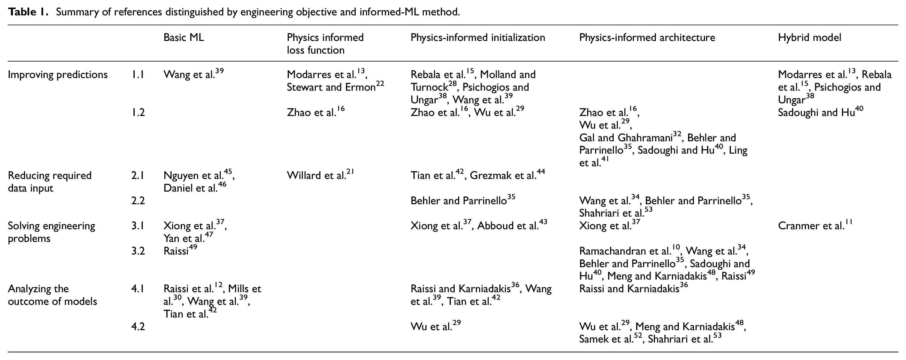
In the context of this review, interpretability has concerned methods that permit meaningful analysis of the model outcomes whereas transparency has been categorized as an inclusion of physical insight into the ML pipeline itself. In reality, these concepts are open to interpretation due to the uncertainty surrounding what constitutes an explainable ML model. One of the most compelling aspects of informed ML, introduced in Section 4.3, is the potential to both solve and discover new causal relationships to a greater precision. Understandably there is often a lack of pre-existing knowledge in situations where this is the objective. Hence, further development is mainly likely to rely on novel architectures that can make use of limited data to guide the starting parameters in order to reduce the domain space. This is highlighted in Table 1 due to the concentration of cases that aim to incorporate informed initialization and informed architecture to achieve this. Another interesting point to note from Table 1, is the number of examples that either incorporate multiple informed ML methods or in some cases achieve multiple engineering objectives. The former is prominent throughout this review, as this will most likely be required to tackle innovative applications of informed-ML in engineering. For example, it would be feasible to incorporate informed loss, informed architecture and informed initialization together, which would both aid generalizability and potentially decrease computational expense by narrowing the search domain. Such an approach would undoubtably lead to increasingly explainable ML models.

Due to its precedence in the field of informed-ML, hybrid modeling is likely to be the most accessible method to a variety of engineering specialists. This is also due to its relative ease of implementation. Hybrid modeling would provide a method to account for missing causal relationships for domains in which there exists a suitable mechanistic model that may not describe the exact nature of the process at hand. This approach would also require relatively limited thought to develop methods that include domain knowledge and which ensure generalizability and physical consistency of the outputs. Unsupervised learning is currently of principal concern throughout the ML community, due to the increasing reliance on large, labeled data sets for training. This is of particular importance in engineering where labeled data can be extremely computationally or experimentally expensive. Informed-ML offers an inherent solution in that data must remain constrained by the same physical principles as the model itself. Therefore, physics informed loss has the potential to remedy these concerns, however further mathematical development of this concept in the case of complex engineering domains is required.

Currently most development is conducted in isolated research areas by individuals working on distinct disciplines. However, for there to be meaningful advancements in this field, future research must form a coordinated effort between computer scientists and engineers. An important pre-requisite, is the development of a common taxonomy for both communities to use. This would streamline the incorporation of physical knowledge into novel ML algorithms by leveraging their differing expertise. This review aims to provide a step toward such a reference framework in order to introduce these concepts to both engineering and computer science communities through the objective to method development path proposed. Similar papers have proposed differing frameworks.^4,5,21 However, at the time of writing, we were not able to discover such a framework specifically concerning informed-ML in engineering. Finally, the uncertainty surrounding a clear definition of explainability must be addressed in the context of engineering. In order to ensure that the safety-critical nature of engineering is respected, it is most likely that a combination of methods must be used to produce end to end informed-ML pipelines that mitigate the risk caused by uncertainty in each aspect of the model. This will ensure greater adoption of these methods throughout engineering in the future.

Conclusions

The purpose of this paper has been to introduce the principal techniques for incorporating physical understanding into machine learning models. By undertaking a review of the literature we have been able to identify the key requirements of this informed or gray box machine learning. In particular, it has been argued that applications in engineering frequently require a model to be explainable. Explainability, in turn, requires an ability to understand the method itself (transparency) and that the output of the model can be explained by reference to established physical (or heuristic) knowledge. This aspect is usually termed “interpretability.” Whilst traditional black box approaches may exhibit elements of each of these characteristics, there is no guarantee that they will do so. Further, traditional approaches of unsupervised learning tend to be “data hungry,” so that a stable model is only produced when trained on a considerable amount of experimental or numerical data. This clearly becomes an issue when experiments or simulation are difficult, time-consuming or expensive.

In the light of these issues, researchers have turned to approaches which capture some of the underlying physics or existing mechanistic understanding. Hence, a selection of the most promising methods for creating physics informed models were introduced and assessed four common engineering requirements, as summarized in Table 1. This allows the reader to easily identify their area of interest.

The simplest approach to implement is probably to use physics-informed initialization. However, whilst this will guide the ML algorithm, there is no guarantee that it will converge to a physically acceptable solution. Using a physics-guided loss function is more complex, but will provide a level of constraint. However there is a danger of forcing the ML solution to conform to the deterministic physics, whereas the data may incorporate factors not captured by the model. A useful alternative in some situations might therefore be hybrid modeling, where the ML approach is used to model aspects of the data that go beyond current physical understanding. Finally, bespoke architectures have their place, but are less accessible to practicing engineers, who may lack the ability to select and implement the appropriate modifications.

It is evident that a combination of methods is most likely to prove effective in order to impose physical insight on a machine learning model. It is argued that this will result in the increased explainability of informed-ML. However, for applications in engineering, an active effort must be made to ensure that both interpretability and transparency are incorporated throughout the ML pipeline using the methods set out in this review. This will allow engineers to benefit from the advantages of ML, while maintaining the physical rigor. For real world applications it is important that engineers can justify their model predictions so that they may be incorporated into design methods, particularly where public safety is involved.

Footnotes

Declaration of conflicting interests

The author(s) declared no potential conflicts of interest with respect to the research, authorship, and/or publication of this article.

Funding

The author(s) received no financial support for the research, authorship, and/or publication of this article.

References

Brunton

Kutz

. Data-driven science and engineering: machine learning, dynamical systems, and control. Cambridge: Cambridge University Press, 2019.

Algorithms

. Accountable algorithms, 2012, pp.1–7.

Guidotti

Monreale

Ruggieri

, et al. A survey of methods for explaining black box models. arXiv 2018; 51: 5.

Von Rueden

Mayer

Beckh

, et al. Informed machine learning-A taxonomy and survey of integrating knowledge into learning systems IEEE Transactions on knowledge and data engineering, Vol 35, No 1, Jan 2023, pp.614–633.

Roscher

Bohn

Duarte

, et al. Explainable machine learning for scientific insights and discoveries. arXiv 2019, 1–29.

Daw

Thomas

Carey

, et al. Physics-guided architecture (PGA) of neural networks for quantifying uncertainty in lake temperature modelling. In: Proc. 2020 SIAM Int. Conf. Data Mining, SDM 2020, SIAM, Philadelphia, PA, 2020, pp.532–540.

McCulloch

Pitts

. A logical calculus of the ideas immanent in nervous activity. Bull Math Biophys 1943; 5(4): 115–133.

Livingstone

Manallack

Tetko

. Data modelling with neural networks: advantages and limitations. J Comput Aided Mol Des 1997; 11(2): 135–142.

Emmert-Streib

Yang

Feng

, et al. An introductory review of deep learning for prediction models with big data. Front Artif Intell 2020; 3: 4–23.

10.

Ramachandran

Zoph

. Searching for activation functions. arXiv 2017, 1–13.

11.

Cranmer

Greydanus

Hoyer

, et al. Agrangian Neural Networks, pp.1–9.

12.

Raissi

Perdikaris

Karniadakis

. Physics informed deep learning (Part II): Data-driven discovery of nonlinear partial differential equations. arXiv 2017; no. Part I: 1–22.

13.

Modarres

Astorga

Droguett

, et al. Convolutional neural networks for automated damage recognition and damage type identification. Struct Control Health Monit 2018; 25(10): e2230.

14.

Karpatne

Watkins

Read

, et al. Physics-guided neural networks (PGNN): An application in lake temperature modelling. arXiv 2017.

15.

Rebala

Ravi

Churiwala

. An introduction to machine learning. Berlin: Springer International Publishing, 2019.

16.

Zhao

Shirvan

Salko

, et al. On the prediction of critical heat flux using a physics-informed machine learning-aided framework. Appl Therm Eng 2020; 164.

17.

Jia

, et al. Physics guided RNNs for modeling dynamical systems: A case study in simulating lake temperature profiles. In: SIAM Int. Conf. Data Mining, SDM 2019, SIAM, Philadelphia, PA, 2019, pp.558–566.

18.

Pfrommer

Zimmerling

Liu

, et al. Optimisation of manufacturing process parameters using deep neural networks as surrogate models. Procedia CIRP 2018; 72: 426–431.

19.

Bikmukhametov

Jäschke

. Combining machine learning and process engineering physics towards enhanced accuracy and explainability of data-driven models. Comput Chem Eng 2020; 138: 1–27. DOI: 10.1016/j.compchemeng.2020.106834

20.

Unknown. What is deep learning and neural network. House of Bots, 2017. https://www.houseofbots.com/news-detail/1442-1-what-is-deep-learning-and-neural-network.

21.

Willard

Jia

, et al. Integrating physics-based modeling with machine learning: a survey. arXiv 2020; 1(1): 1–34.

22.

Stewart

Ermon

. Label-free supervision of neural networks with physics and domain knowledge. In: 31st AAAI Conf. Artif. Intell. AAAI 2017, Assoc. for Advancement of Artificial Intelligence, Palo Alto, CA, 2017, vol. 1, no. 1, pp.2576–2582.

23.

Haghighat

Raissi

Moure

, et al. A physics-informed deep learning framework for inversion and surrogate modeling in solid mechanics. Comput Methods Appl Mech Eng 2021; 379.

24.

Abadi

Barham

Chen

, et al. TensorFlow: A system for large-scale machine learning. In: 12th USENIX Symposium on Operating Systems Design and Implementation (OSDI 16), USENIX Association, Savannah, GA, 2016, pp.265–283.

25.

Abueidda

Koric

. Meshless physics-informed deep learning method for three-dimensional solid mechanics. Int J Numer Methods Eng 2021; 122: 7182–7201.

26.

Elhamod

, et al. CoPhy-PGNN: learning physics-guided neural networks with competing loss functions for solving eigenvalue problems, 2020, http://arxiv.org/abs/2007.01420.

27.

Karpatne

Atluri

Faghmous

, et al. Theory-guided data science: A new paradigm for scientific discovery from data. IEEE Trans Knowl Data Eng 2017; 29(10): 2318–2331.

28.

Molland

Turnock

. Marine rudders and control surfaces. Oxford: Butterworth-Heinemann, 2007.

29.

Wang

Xiao

, et al. A priori assessment of prediction confidence for data-driven turbulence modeling. Flow Turbul Combust 2017; 99(1): 25–46.

30.

Mills

Spanner

Tamblyn

. Publisher's note: deep learning and the schrödinger equation. Phys Rev A 2018; 97: 042113.

31.

Wang

Kumar

Shelton

, et al. Harnessing deep neural networks to solve inverse problems in quantum dynamics: machine-learned predictions of time-dependent optimal control fields. Phys Chem Chem Phys 2020; 22: 22889–22899.

32.

Gal

Ghahramani

. Dropout as a Bayesian approximation: Representing model uncertainty in deep learning. In: 33rd Int. Conf. Mach. Learn. ICML 2016, JMLR.org, 2016, vol. 3, pp.1651–1660.

33.

Muralidhar

Cao

, et al. Physics-guided deep learning for drag force prediction in dense fluid-particulate systems. Big Data 2020; 8(5): 431–449.

34.

Wang

Walters

. Incorporating symmetry into deep dynamics models for improved generalization. arXiv 2020.

35.

Behler

Parrinello

. Generalized neural-network representation of high-dimensional potential-energy surfaces. Phys Rev Lett 2007; 98(14): 146401–146404.

36.

Raissi

Karniadakis

. Hidden physics models: machine learning of nonlinear partial differential equations. J Comput Phys 2018; 357: 125–141.

37.

Xiong

, et al. Data-driven discovery of partial differential equations for multiple-physics electromagnetic problem. arXiv 2019; April: 1–7.

38.

Psichogios

Ungar

. A hybrid neural network-first principles approach to process modeling. AIChE J 1992; 38(10): 1499–1511.

39.

Wang

Ling

, et al. A comprehensive physics-informed machine learning framework for predictive turbulence modelling. arXiv 2017; 074602: 1–28.

40.

Sadoughi

. A physics-based deep learning approach for fault diagnosis of rotating machinery. In: Proc. IECON 2018 - 44th Annu. Conf. IEEE Ind. Electron. Soc., IEEE, New York, NY, 2018, pp.5919–5923.

41.

Ling

Jones

Templeton

. Machine learning strategies for systems with invariance properties. J Comput Phys 2016; 318: 22–35.

42.

Tian

Morillo

Azarian

, et al. Motor bearing fault detection using spectral kurtosis-based feature extraction coupled with K-nearest neighbor distance analysis. IEEE Xplore, https://ieeexplore.ieee.org/stamp/stamp.jsp?tp=&arnumber=7360161 (2016, accessed 31 August 2021).

43.

Abboud

Antoni

Sieg-Zieba

, et al. Envelope analysis of rotating machine vibrations in variable speed conditions: A comprehensive treatment. Mech Syst Signal Process 2017; 84: 200–226.

44.

Grezmak

Zhang

Wang

, et al. Interpretable convolutional neural network through layer-wise relevance propagation for machine fault diagnosis. IEEE Sens J 2020; 20(6): 3172–3181.

45.

Nguyen

Barhli

Muñoz

, et al. Computer vision with error estimation for reduced order modeling of macroscopic mechanical tests. Complexity; 2018: 1–10. DOI: 10.1155/2018/3791543.

46.

Daniel

Casenave

Akkari

, et al. Model order reduction assisted by deep neural networks (ROM-net). Adv Model Simul Eng Sci 2020; 7(1): 1–27 DOI: 10.1186/s40323-020-00153-6

47.

Yan

Yang

, et al. Bayesian migration of Gaussian process regression for rapid process modeling and optimization. Chem Eng J 2011; 166(3): 1095–1103.

48.

Meng

Karniadakis

. A composite neural network that learns from multi-fidelity data: application to function approximation and inverse PDE problems, no. 1, pp.1–29.

49.

Raissi

. Deep hidden physics models: deep learning of nonlinear partial differential equations. J Mach Learn Res 2018; 19: 1–24.

50.

Long

Dong

. PDE-Net 2.0: learning PDEs from data with a numeric-symbolic hybrid deep network. J Comput Phys 2019; 399: 108925.

51.

Rackauckas

, et al. Universal differential equations for scientific machine learning. arXiv 2020.

52.

Samek

Binder

Montavon

, et al. Evaluating the visualization of what a deep neural network has learned. IEEE Trans Neural Netw Learn Syst 2017; 28(11): 2660–2673.

53.

Shahriari

Swersky

Wang

, et al. Taking the human out of the loop: A review of Bayesian optimization. Proc IEEE 2016; 104(1): 148–175.

54.

Yang

Perdikaris

. Adversarial uncertainty quantification in physics-informed neural networks. J Comput Phys 2019; 394: 136–152.

55.

Singh

Duraisamy

. Using field inversion to quantify functional errors in turbulence closures. Phys Fluids 2016; 28(4): 045110.

Informed machine learning methods for application in engineering: A review

Abstract

Keywords

Introduction

Background

Terminology

Historical Context

Fundamental Principles of Neural Networks

Modeling the artificial neuron

Activation function

Loss function

Neural network architecture

Physics informed ML methods

Physics informed loss function

Physics informed initialization

Physics informed architecture

Intermediate physical variables

Encoding invariances, symmetries and domain specific knowledge

Physics informed Gaussian process regression

Hybrid modeling

Incorporating informed ML in engineering

Improving predictions beyond traditional models

Outcome interpretability leading to increased explainability

Applications that allow for outcome interpretability and basic model transparency

Reducing Model Data Requirements

Outcome interpretability leading reduced model data requirements

Applications with model transparency leading to reduced model data requirements

Solving Engineering Problems

Outcome interpretability used for solving problems in engineering

Applications with model used for solving problems in engineering

Analysis of the resulting model outcomes

Outcome interpretability used for analysis of informed-ML outputs

Applications that use model transparency for analysis of informed-ML outputs

Discussion

Conclusions

Footnotes

Declaration of conflicting interests

Funding

References