Rapid analysis of the effects of surface and sub-surface defects in elastohydrodynamic contacts

Abstract

Surface and sub-surface defects alter the stress distribution in the material and tend to significantly reduce the life of elastohydrodnamic (EHL) contacts. Where the defects lie well below the surface their effect may be obtained by taking the EHL pressures from standard analyses and using these to determine the stress distribution. However, defects lying closer to the surface can produce significant local displacements and alter the EHL pressures. Analysis is difficult because these displacements change as the defect passes under the conjunction and calculation tends to be extremely time consuming. This paper presents an extension to the perturbation technique used for the rapid analysis of surface roughness. This extension enables solutions for both two and three dimensional defects to be obtained rapidly. The procedure is outlined and a number of examples given.

Introduction

Surface and sub-surface defects such as cracks and inclusions tend to reduce the life of elastohydrodynamic components and may lead to catastrophic failure. The effect of inclusions has received considerable attention in recent years, see for example,^1–15 but detailed analysis is hampered by the complexity of the problem. Behaviour of surface defects, typically cracks, is perhaps even more complex with crack propagation being influenced by the presence of fluid inside the defect itself. There is a very considerable body of theoretical and experimental work, see, again, for example,^16–25 on this topic. However, it is not the intention of this paper to examine the effect of surface and sub-surface defects in detail but simply to present a procedure that allows its rapid evaluation.

For inclusions the simplest solution is simply to take the pressure distribution from an elastohydrodynamic (EHL) analysis for a surface without any imperfections (denoted as smooth in this paper for brevity) and use that to find the stresses. This produces acceptable results unless the defect is on, or close to, the surface in which case the surface deformations can significantly affect the EHL pressures and modify the stress distribution. This paper considers those situations where surface deformations are important.

Most existing analyses of this problem and those for surface cracks directly couple the lubrication calculation with an elastic analysis of the sub-surface region and tend to be very lengthy, particularly when the surface with the defect is moving. Part of the problem is that, in order to obtain an accurate solution, it is necessary to use fairly small time steps and this requires the elasticity problem to be solved many times.

Recently, the author developed a rapid perturbation method for the analysis of low amplitude roughness in EHL contacts^26,27 and it has proved possible to extend this to examine the effect of surface and sub-surface imperfections. This enables solutions to be obtained in a far shorter time than using current procedures.

The analysis requires three steps. First, the elasticity problem needs to be simplified so that the relationship between surface displacements and the surface pressures is replaced by the standard relationship for homogeneous half spaces plus a local flexibility matrix around the defect (or defects). This local flexibility matrix moves with the surface containing the defect. Second, the effect of sinusoidal roughness needs to be determined. This uses a modification of the analysis given in Hooke and Morales-Espejel. ²⁶ Third, the two need to be combined to obtain results for the pressures and clearances in the contact as the defect moves through the conjunction. The resulting pressures may then be used to estimate the stresses.

The process effectively separates the elastic analysis of the surfaces from the EHL problem so only a single elastic analysis is required for a given type of defect whatever the lubrication conditions and only a single EHL analysis is needed for all types of defect.

The analysis is limited to line contacts, although the sub-surface structures may be three-dimensional, but, since most practical conjunctions approximate to line contacts, this restriction is unlikely to be of major practical significance. In addition, it was shown in Hooke and Venner ²⁸ that the behaviour of roughness in line and point conjunctions is very similar and this allows the results to be applied to other conjunctions, notably to the point contact used in many experimental tests. Finally, the EHL analysis given in Hooke and Morales-Espejel^26,27 includes thermal effects. Since these can be incorporated without significant time penalty they are included in the current results.

For simplicity it will be assumed that both surfaces move normal to the contact and that the transverse velocities are zero. Transverse motion is included in Hooke and Morales-Espejel^26,27 and the extension to include it is straightforward.

The aim of the current paper is to outline the use of the perturbation analysis in the solution of this type of EHL problem and although a number of examples are included these are intended, primarily, to illustrate the procedure. Accordingly, relatively simple geometric imperfections are considered as shown in Figure 1(a) and (b). Both are artificial. The first because no defect is likely to be geometrically perfect; the second makes the assumption that crack sides remain in contact – valid for vertical cracks because the horizontal stresses are compressive under the conjunction – but ignores the effect of friction. In addition only two different operating conditions, given in Table 1, are considered.

Figure 1.

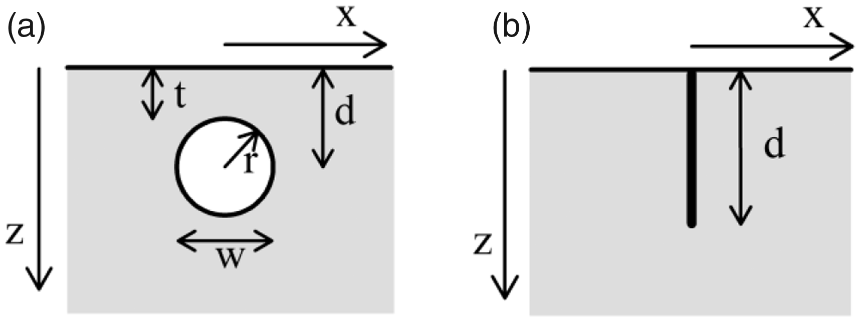
(a) Cylindrical or spherical defect; (b) frictionless, vertical crack.

Table 1.

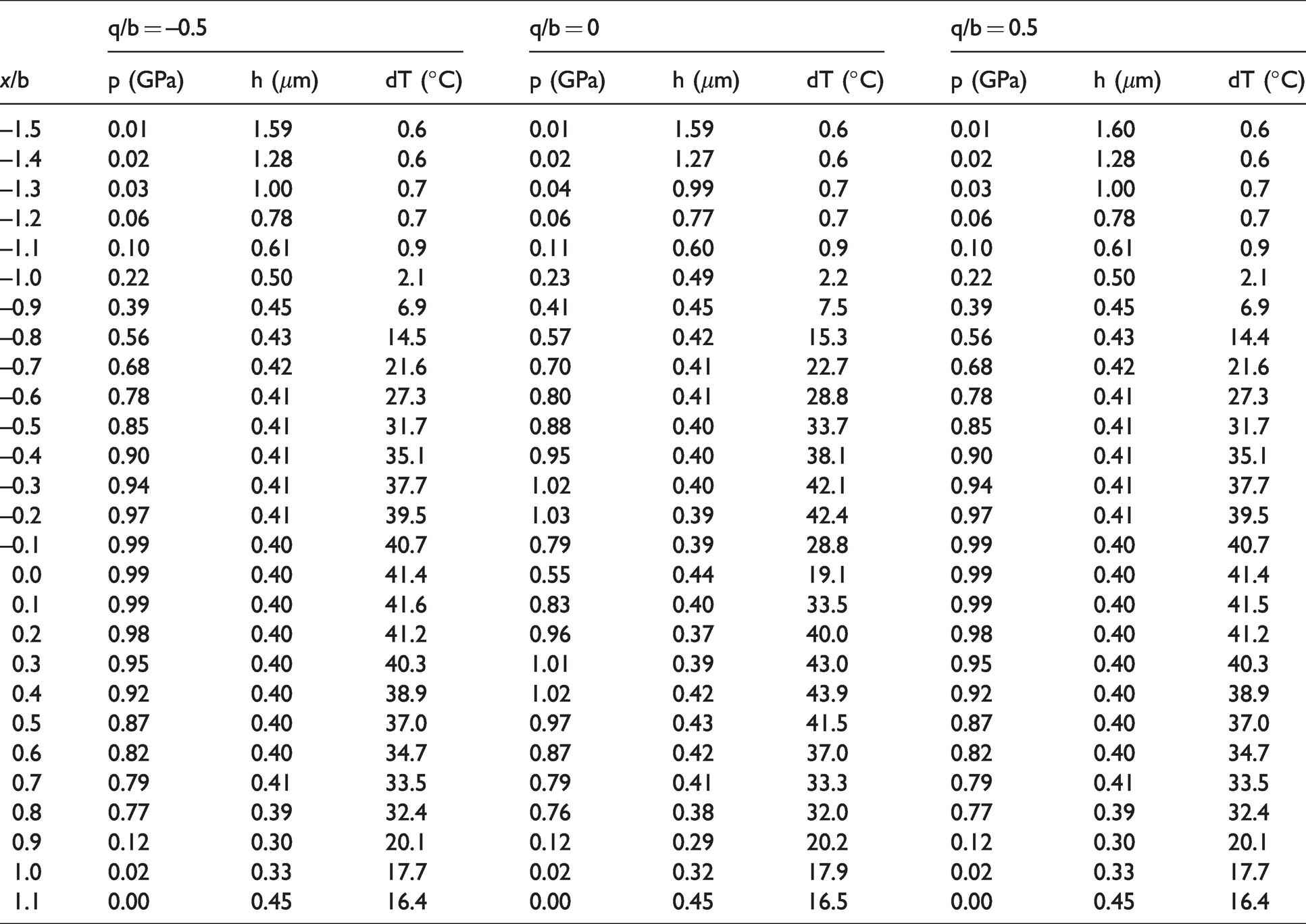
Fluid properties and operating conditions.

Hertz pressure	1 GPa
Equivalent radius	10 mm
Elastic moduli	206 GPa
Poisson’s ratio	0.3
Semi Hertz width	0.177 mm
Thermal conductivity of surfaces	46 W/m/K
Density of surfaces	7.85 Mg/m3
Specific heat of surfaces	470 J/kg/K
Roelands fluid
Viscosity at room pressure and 30 °C	50 mPa s
Pressure viscosity coefficient	21/GPa
Temperature viscosity coefficient	0.06/K
Fluid compressibility Dowson–Higginson
Initial gradient	0.6/GPa
High pressure density ratio	1.353
Temperature density coefficient	0.00065/K
Power law shear stress – shear strain rate – $\eta \dot{\gamma }=\tau {\left[1+{\left(\frac{\tau }{\mathrm{S}}\right)}^n\right]}^{\mathrm{a}}$	S = 5 MPa, n = 2, a = 0.6
Specific heat of fluid	2000 J/kg/K
Density of fluid	875 kg/m3
Thermal conductivity of fluid	0.14 W/m/K
Inlet temperatures	30 °C
Mean surface velocity	1.5/ms
Velocity difference for sliding contact	1/ms (SRR = 0.667)

Table 2.

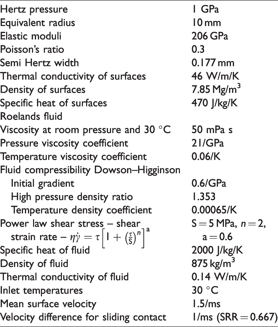
Tabulated results.

x/b	q/b = –0.5			q/b = 0			q/b = 0.5
	p (GPa)	h (μm)	dT (°C)	p (GPa)	h (μm)	dT (°C)	p (GPa)	h (μm)	dT (°C)
–1.5	0.01	1.59	0.6	0.01	1.59	0.6	0.01	1.60	0.6
–1.4	0.02	1.28	0.6	0.02	1.27	0.6	0.02	1.28	0.6
–1.3	0.03	1.00	0.7	0.04	0.99	0.7	0.03	1.00	0.7
–1.2	0.06	0.78	0.7	0.06	0.77	0.7	0.06	0.78	0.7
–1.1	0.10	0.61	0.9	0.11	0.60	0.9	0.10	0.61	0.9
–1.0	0.22	0.50	2.1	0.23	0.49	2.2	0.22	0.50	2.1
–0.9	0.39	0.45	6.9	0.41	0.45	7.5	0.39	0.45	6.9
–0.8	0.56	0.43	14.5	0.57	0.42	15.3	0.56	0.43	14.4
–0.7	0.68	0.42	21.6	0.70	0.41	22.7	0.68	0.42	21.6
–0.6	0.78	0.41	27.3	0.80	0.41	28.8	0.78	0.41	27.3
–0.5	0.85	0.41	31.7	0.88	0.40	33.7	0.85	0.41	31.7
–0.4	0.90	0.41	35.1	0.95	0.40	38.1	0.90	0.41	35.1
–0.3	0.94	0.41	37.7	1.02	0.40	42.1	0.94	0.41	37.7
–0.2	0.97	0.41	39.5	1.03	0.39	42.4	0.97	0.41	39.5
–0.1	0.99	0.40	40.7	0.79	0.39	28.8	0.99	0.40	40.7
0.0	0.99	0.40	41.4	0.55	0.44	19.1	0.99	0.40	41.4
0.1	0.99	0.40	41.6	0.83	0.40	33.5	0.99	0.40	41.5
0.2	0.98	0.40	41.2	0.96	0.37	40.0	0.98	0.40	41.2
0.3	0.95	0.40	40.3	1.01	0.39	43.0	0.95	0.40	40.3
0.4	0.92	0.40	38.9	1.02	0.42	43.9	0.92	0.40	38.9
0.5	0.87	0.40	37.0	0.97	0.43	41.5	0.87	0.40	37.0
0.6	0.82	0.40	34.7	0.87	0.42	37.0	0.82	0.40	34.7
0.7	0.79	0.41	33.5	0.79	0.41	33.3	0.79	0.41	33.5
0.8	0.77	0.39	32.4	0.76	0.38	32.0	0.77	0.39	32.4
0.9	0.12	0.30	20.1	0.12	0.29	20.2	0.12	0.30	20.1
1.0	0.02	0.33	17.7	0.02	0.32	17.9	0.02	0.33	17.7
1.1	0.00	0.45	16.4	0.00	0.45	16.5	0.00	0.45	16.4

It is clear that defects well below the surface do not affect the EHL pressures and can be examined using the smooth EHL results. Equally those near the surface do and require a full analysis. There is, at present, little information about the transition depth. Although too few examples are considered in this paper to provide a definitive answer, the effect of depth is considered for two geometrically simple defects and the results may, possibly, provide some guidance.

Elastic behaviour

In numerical EHL analyses the pressures, p, and the surface displacements, w, will typically be defined at a number of points and, in the absence of any surface defects, the displacements will be obtained using a relationship for the combined surfaces of the form

$$\mathrm{w}={\mathrm{K}}_{\mathrm{h}}\mathrm{p}$$

(1)

where K_h is some matrix that relates the displacements, w, to the pressures, p, for half spaces.

The coefficients of the matrix can either be explicit or may be implicit if, for example, Fourier transform methods are used to evaluate the distortions.

When defects are present, this relationship will be modified and will become

$$\mathrm{w}=\left[{\mathrm{K}}_{\mathrm{h}}+{\mathrm{K}}_{\mathrm{d}}\right]\mathrm{p}$$

(2)

where the perturbation matrix, K_d, represents the change in the pressure-clearance relationship introduced by the defects. For isolated inclusions or surface imperfections the modification K_d will be localised to the defect and it is convenient to divide the calculation of the surface displacements into a calculation of the overall displacements, using K_h, and then modify these using K_d to obtain the total displacements. This has the advantage that the matrix K_d needs to be determined only once, even when the location of the defect changes, and avoids the need for a full elastic analysis at each step of any EHL calculation.

Figure 2 illustrates the process for a cylindrical void passing under a contact subject to a Hertzian pressure. The deflections from K_h and K_d are calculated separately and summed to obtain the total displacement.

Figure 2.

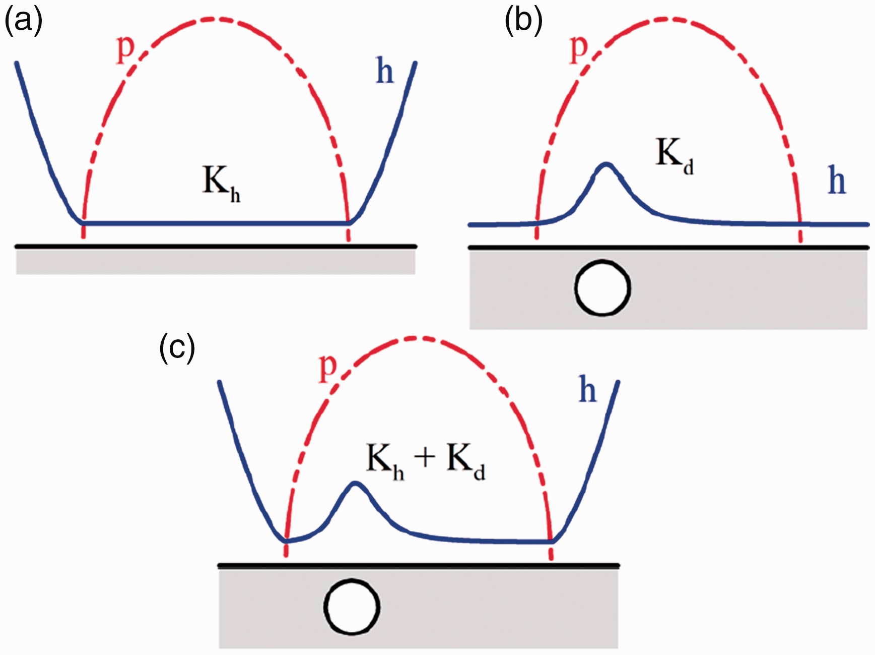
Combination of Hertzian displacements and local defections from the defect.

Calculation of the perturbation matrix, K_d

The simplest way to obtain the perturbation matrix, K_d, is to use either a finite element or (primarily for surface cracks) a boundary element analysis, although other methods are possible. Details will obviously vary but it should be possible to obtain a matrix relating the surface loadings to the surface deformations with a single solution either by using simultaneous multiple loadings or, for finite elements, standard sub-structure facilities. The resulting matrix will contain both K_d and an approximation to the half space behaviour which needs to be removed. A repetition of the analysis using the same mesh but with the defect absent (typically achieved by setting the defect moduli to those of the base material) should yield the required approximation to the half space behaviour. Subtraction yields K_d. Other methods of eliminating the half space approximation are possible but repeating the analysis appears simplest.

The analysis will necessarily use an extended region and the calculated matrix K_d will contain many zero, or near zero, coefficients for points distant from the defect. These may be trimmed to produce a compact matrix relating the surface loads and displacements for just the region around the defect.

All the examples given in this paper were obtained using finite elements and details are given in Appendix 2. As an example of the perturbation matrix, K_d, Figure 3(a) shows the displacements produced by a cylindrical inclusion under uniform loading for different defect moduli, while Figure 3(b) shows the effect of pressure adjacent to a vertical, frictionless crack in the surface.

Figure 3.

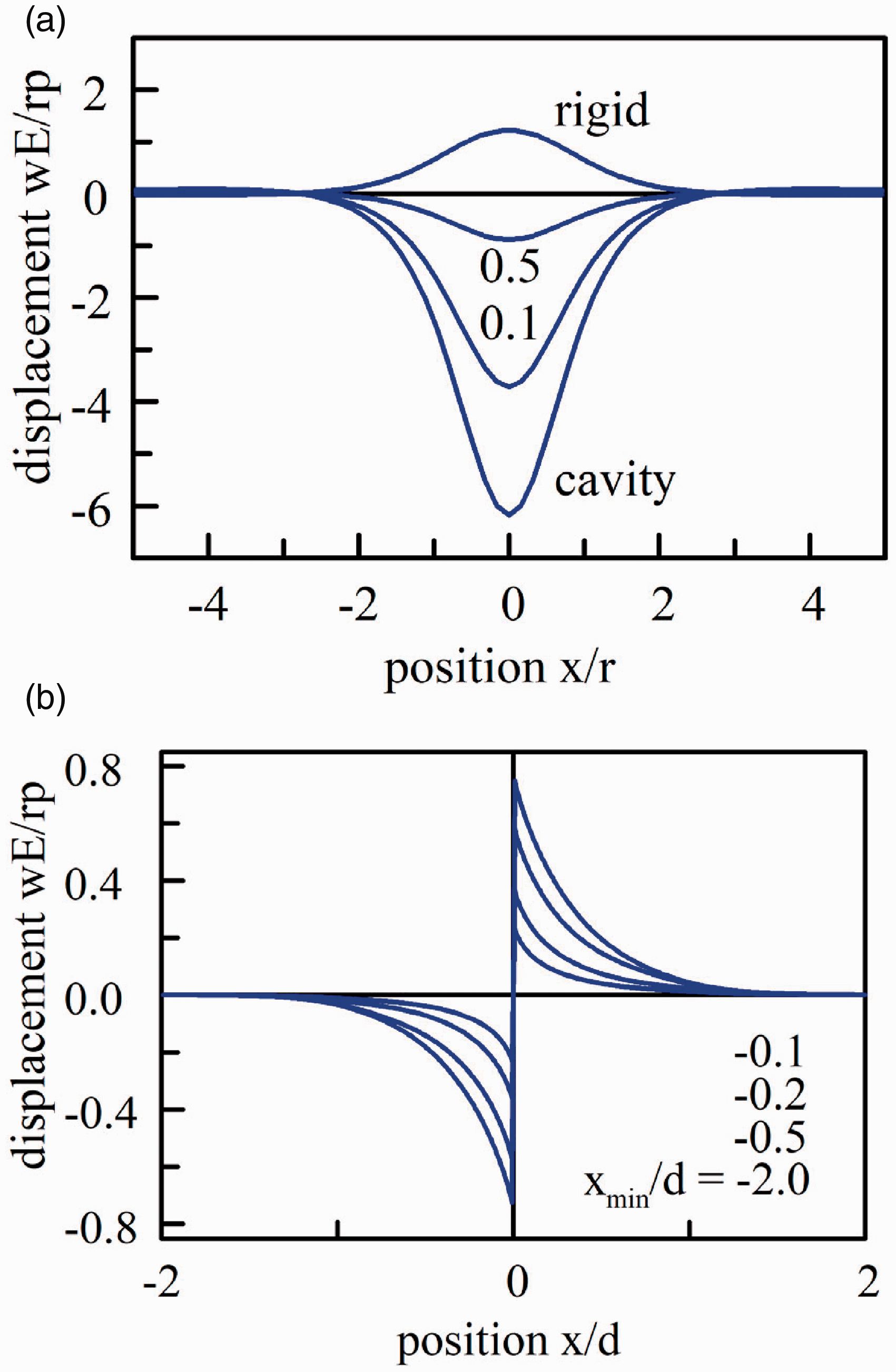
(a) Modifications to deflections produced by a uniform pressure on a cylindrical inclusion of radius, r, centred at a depth of 1.5r below the surface. The numerical values give the ratio of the inclusion modulus to that of the bulk material; (b) effect of a vertical, frictionless crack of depth d. The curves show the displacements produced by a uniform pressure acting from x_min to the edge of the crack.

It was assumed that the sides of the crack remained in contact. The curves are skew symmetric since any symmetric pressure distribution will produce identical displacements in a half space both with and without the defect.

A similar result for a spherical void is shown in Figure 4. It may be noted that the maximum deformation is far lower than for a cylindrical void of the same dimensions.

Figure 4.

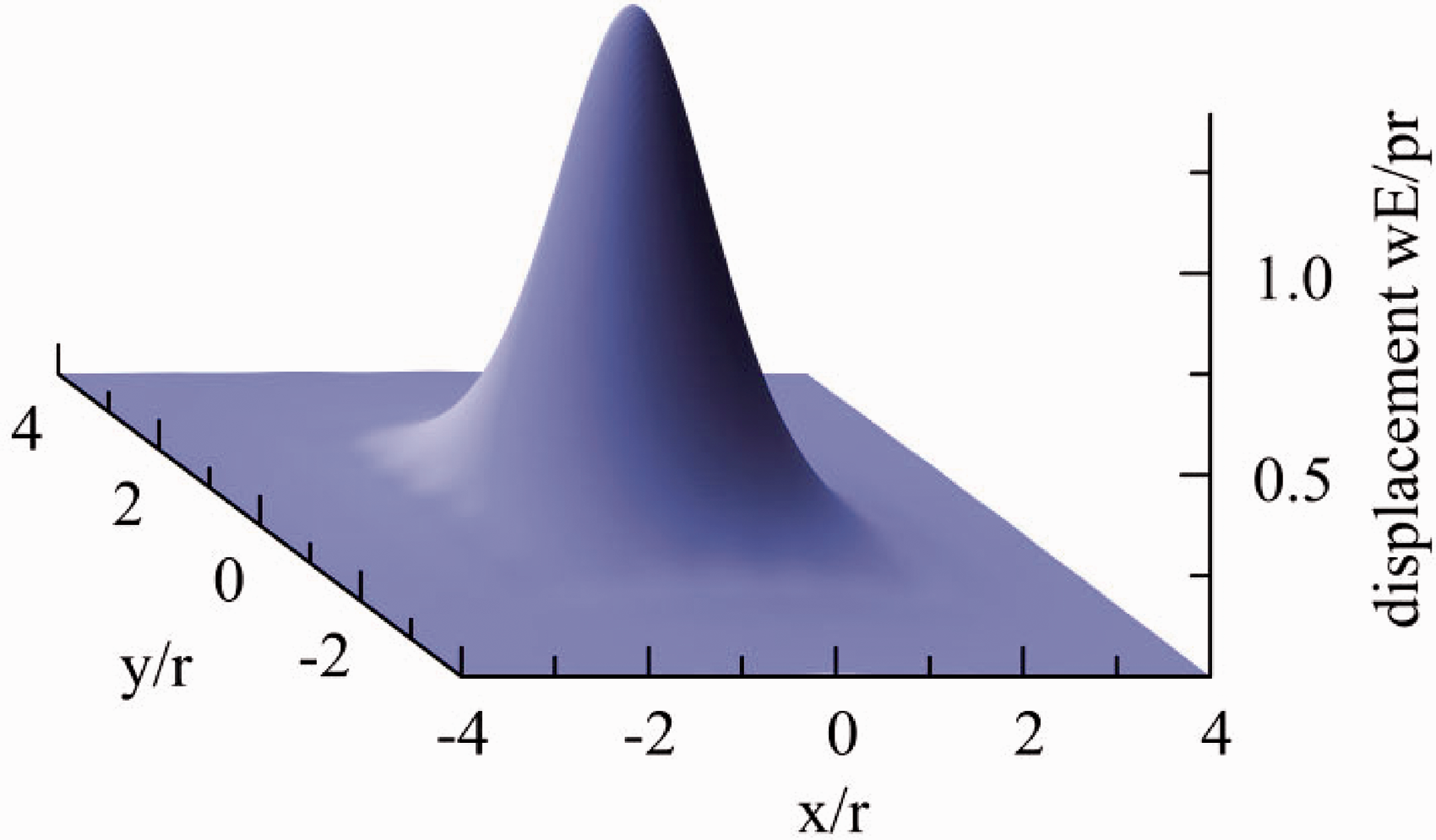
Modifications to deflections produced by a uniform pressure on a spherical void at a depth of 1.5r below the surface.

In general the nodes of the flexibility matrix, K_d, will not coincide with those of the EHL analysis and it is necessary to integrate the EHL pressures to obtain the loads on the nodes of the flexibility grid. Interpolation between the displacements of the K_d mesh gives the values on the EHL grid. Provided both grids are reasonably fine, linear interpolation appears adequate and, if linear finite elements are used, is necessary to satisfy the FE energy conditions.

The perturbation matrices were calculated using a defect of unit size and a modulus of 1. Scaling gives the flexibility perturbation for any geometrically similar defect.

EHL behaviour

In ²⁶ the behaviour of low amplitude, surface roughness of the form

$$\exp \left[\mathrm{i}\mathrm{\omega }\mathrm{x}\right]\mathrm{ }\exp \left[\mathrm{i}\text{ξ}\mathrm{y}\right]\mathrm{ }\exp \left[\mathrm{i}\mathrm{\chi }\mathrm{t}\right]$$

(3)

was examined and it was shown that this would produce pressure, clearance and temperature changes with the form, for example for the pressure perturbation, of

$$\widehat{\mathrm{P}}\left(\mathrm{x}\right)\mathrm{ }\exp \left[\mathrm{i}\text{ξ}\mathrm{y}\right]\mathrm{ }\exp \left[\mathrm{i}\mathrm{\chi }\mathrm{t}\right]$$

(4)

where $\widehat{\mathrm{P}}$ (x) is complex.

For surface roughness, where the roughness moves, unchanged, with the surface, χ and ω are related by the surface velocity

$$\chi =\text{–}{\mathrm{u}}_1\omega$$

(5)

However, the analysis is general and can be used, without any changes, for the wider range of values of χ needed for the analysis of defects. Full details of how the response to roughness of the form of equation (3) is obtained are given in Hooke and Morales-Espejel ²⁶ and a brief outline is included in Appendix 3.

As examples, Figure 5(a) and (b) show typical examples of the behaviour for rolling and sliding contacts. With the rolling contact, thermal and shear effects are small and the fluid film generated in the inlet passes through the conjunction, with little change, at the mean surface velocity. In the inlet the original roughness is reduced in amplitude but additional variations are produced by the difference of χ from –u₁ω – the ψ term in equation (6). Thus the final clearance perturbation is the sum of two components that each vary sinusoidally with x. Because the pressure perturbation is directly relate to the change in clearance its variation follows a similar pattern. However, in the absence of sliding, the temperature rise is small and the behaviour is essentially isothermal. The actual behaviour depends heavily on details of the fluid’s properties and in particular on the variation of viscosity with pressure.

Figure 5.

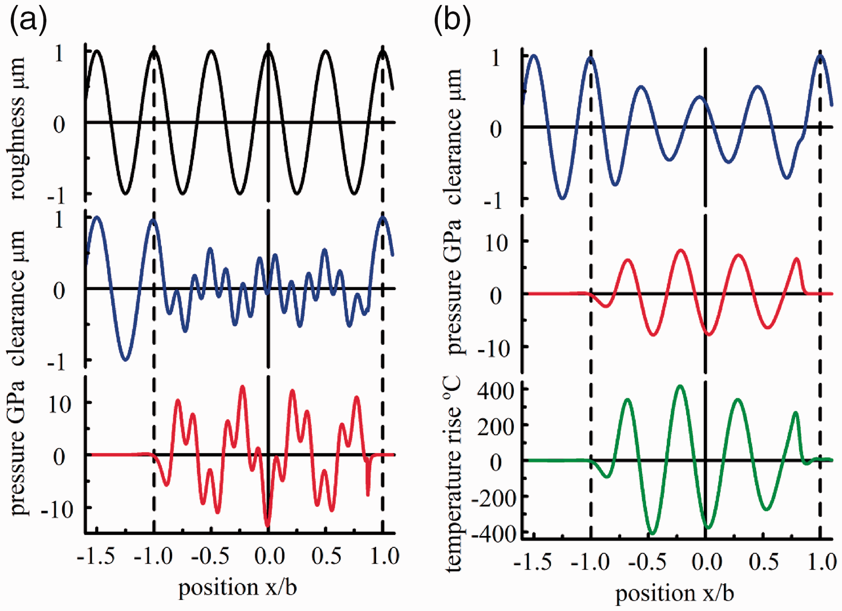
Response to roughness of the form of equation (3). (a) Rolling contact. ωb = 4π, ξb = 10π, χb = –21π, (ψb = –10π). (b) Sliding contact. ωb = 4π, ξb = 10π, χb = –14π, ψb = –10π. Only the real components are shown.

With the sliding contact, thermal and shear properties of the fluid reduce the effective viscosity and the inlet generated wave decays extremely rapidly. However hydrodynamic pressures, generated by the relative sliding of the surfaces, attenuate the roughness. Again the behaviour depends heavily on details of the fluid's properties

To be of any practical use, solutions of the form of equation (4) must be obtained and stored in a form that allows accurate interpolation between a limit set of wave numbers. In addition, the variation with x also needs to be defined using a restricted number of data points. The procedure used in Hooke and Morales-Espejel ²⁷ and adopted in a modified form here was to re-write equation (4) as

$$\widehat{\mathrm{P}}\left(x\right)\exp \left[\mathrm{i}\omega x\right]\exp \left[\mathrm{i}\text{ξ}y\right]\exp \left[\mathrm{i}\left(\psi -\omega \right){\mathrm{u}}_1\mathrm{t}\right]$$

(6)

where ψ arises from the variation in roughness amplitude as the defect moves through the conjunction. Because of the inclusion of the $\exp \left[\mathrm{i}\omega x\right]\mathrm{ }$ term, $\widehat{\mathrm{P}}\left(x\right)$ varies relative slowly with x allowing it to be accurately interpolated from its values at a limited number of points, typically around 50, across the conjunction

$$\widehat{\mathrm{P}}\left(x\right)=\mathrm{ }\sum _{\mathrm{k}}{{\mathrm{N}}_{\mathrm{k}}\left(x\right)\mathrm{ }\widehat{\mathrm{P}}}_{\mathrm{k}}$$

(7)

Simple, local cubic interpolation functions, N_k(x) were used, maintaining slope continuity at the interpolation points, x_k.

Solutions were obtained for an evenly spaced grid of values of ω, ξ and ψ. The maximum and minimum values of these were chosen to cover the full range of expected values and the intervals selected to ensure a maximum interpolation error of below 2%. The results were stored for later retrieval and use.

Perturbation

The presence of the defect alters the surface deformation and, hence, the pressures in the EHL contact. Writing p_s for the pressures without the defect and p_d for the pressure changes produced by the defect, the surface deformation may be expressed as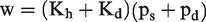

$$\mathrm{w}=\left({\mathrm{K}}_{\mathrm{h}}+{\mathrm{K}}_{\mathrm{d}}\right)\left({\mathrm{p}}_{\mathrm{s}}+{\mathrm{p}}_{\mathrm{d}}\right)$$

$${=\mathrm{ }\mathrm{K}}_{\mathrm{h}}{\mathrm{p}}_{\mathrm{s}}+{\mathrm{K}}_{\mathrm{d}}{\mathrm{p}}_{\mathrm{s}}+{\mathrm{K}}_{\mathrm{h}}{\mathrm{p}}_{\mathrm{d}}+{\mathrm{K}}_{\mathrm{d}}{\mathrm{p}}_{\mathrm{d}}$$

(8)

or:

$${\mathrm{w}=\mathrm{w}}_{\mathrm{s}}+{\mathrm{K}}_{\mathrm{h}}{\mathrm{p}}_{\mathrm{d}}+\mathrm{r}$$

(9)

where w_s is the deformation under smooth conditions and

$$\mathrm{r}={\mathrm{K}}_{\mathrm{d}}{\mathrm{p}}_{\mathrm{s}}+{\mathrm{K}}_{\mathrm{d}}{\mathrm{p}}_{\mathrm{d}}$$

Equation (9) is equivalent to a Hertzian contact with a surface roughness r; the problem analysed in Hooke and Morales-Espejel. ²⁷ However, in the present case the roughness, r, does not simply move with the surface but also changes in form during its transition through the contact. Assuming, for the moment, that the changes to the pressure and flexibility are relatively small, the product ${\mathrm{K}}_{\mathrm{d}}{\mathrm{p}}_{\mathrm{d}}$ can be ignored allowing r to be determined from the smooth EHL pressures alone. Inclusion of the ${\mathrm{K}}_{\mathrm{d}}{\mathrm{p}}_{\mathrm{d}}$ term will be discussed later in the “Inclusion of the K_dp_d term” section.

As an example Figure 6(a) shows the roughness r calculated as a defect passes under an EHL conjunction. Details of the operating conditions are given in Table 1. For clarity the changes have been superimposed on the smooth EHL profile. The amplitude of the roughness, r, grows from zero outside the contact, attaining its maximum value near the centre before decreasing to zero as the defect leaves the conjunction.

Figure 6.

(a) Profile changes produced by a cylindrical void of r/b = 0.1, depth 1.5r. (b) profile changes produced by a vertical, frictionless crack of depth 0.7b. Deformations are calculated using the pressures under a smooth rolling contact.

Figure 6(b) shows a similar result for a vertical crack. Here, displacements are largest when the crack is near the contact ends, zero outside the conjunction but also falling to zero at its centre. This is because the deformation depends largely on the pressure gradient rather than the pressure.

Alternative plots are shown in Figure 7(a) and (b) which show more clearly how the roughness varies with position relative to the defect and with the location of the defect. It may be noted that in both cases the variation in amplitude with the defect location, q, is reasonably smooth. This implies that a relatively coarse spacing of points in the q direction will adequately define the profile in that direction. In turn this limits the range of values of ψ required in equation (6).

Figure 7.

(a) Variation of surface perturbation with defect position, q, and the distance from the defect centre, s. Rolling contact with a cylindrical void of size r/b = 0.1, depth 1.5r; (b) variation of surface perturbation with defect position. Rolling contact with a crack of depth d/b = 0.7.

For a given defect location, q, the roughness, r, is most conveniently defined as a function of s and y, the distances from the centre of the defect in the x and y directions respectively. Since the profile changes with the location of the defect, q, its amplitude r may be written as $\mathrm{r}\mathrm{ }=\mathrm{ }\mathrm{r}\left(\mathrm{s},\mathrm{ }\mathrm{y},\mathrm{ }\mathrm{q}\right)$ (10)

A Fourier transform converts this into components having the form

$$\widehat{\mathrm{R}}\exp \left[\mathrm{i}\omega \mathrm{s}\right]\exp \left[\mathrm{i}\text{ξ}\mathrm{y}\right]\exp \left[\mathrm{i}\psi \mathrm{q}\right]$$

(11)

and noting that x = q +s, this may be converted to

$$\widehat{\mathrm{R}}\exp \left[\mathrm{i}\omega \mathrm{x}\right]\exp \left[\mathrm{i}\text{ξ}\mathrm{y}\right]\exp \left[\mathrm{i}(\psi -\omega ){\mathrm{u}}_1\mathrm{t}\right]$$

(12)

Multiplication of this by the results of the sinusoidal EHL analysis of the “EHL behaviour” section produces values of the perturbations at the integration points x_k as, for example, ${\widehat{\mathrm{P}}}_{\mathrm{k}}$ . Summation using

$$\widehat{\mathrm{P}}\left(x\right)=\sum _{\mathrm{k}}{{\mathrm{N}}_{\mathrm{k}}\left(x\right)\widehat{\mathrm{P}}}_{\mathrm{k}}$$

(13)

enables the Fourier component of pressure for these values of ω, ξ and ψ to be obtained for any value of x. Inverse transforms give the perturbations in the form, for example, of

$$\mathrm{p}\left(x\right)=\sum _{\mathrm{k}}{\mathrm{N}}_{\mathrm{k}}\left(x\right){\mathrm{p}}_{\mathrm{k}}\left(\mathrm{s},\mathrm{ }\mathrm{y},\mathrm{ }\mathrm{q}\right)$$

(14)

From this it is straightforward to find the perturbations for any given values of x, y and q.

The process appears complicated but consists of the repetition of a number of simple steps. First, the roughness, r is calculated as a function of s, y and q. A Fourier transform converts this into components of ω, ξ and ψ. These components are scaled by the stored results of the “EHL behaviour” section for each interpolation point. Inverse transforms give the values at each interpolation point. Finally summation enables the behaviour to be found for any defect location and position. Thus, typically one forward Fourier transform and around 300 inverse transforms are required.

It may be noted that a single analysis yields results that can be interpolated for any values of s, y and q. Because q defines the defect’s location the solution gives the clearances, pressures and temperatures across the conjunction at any specified time.

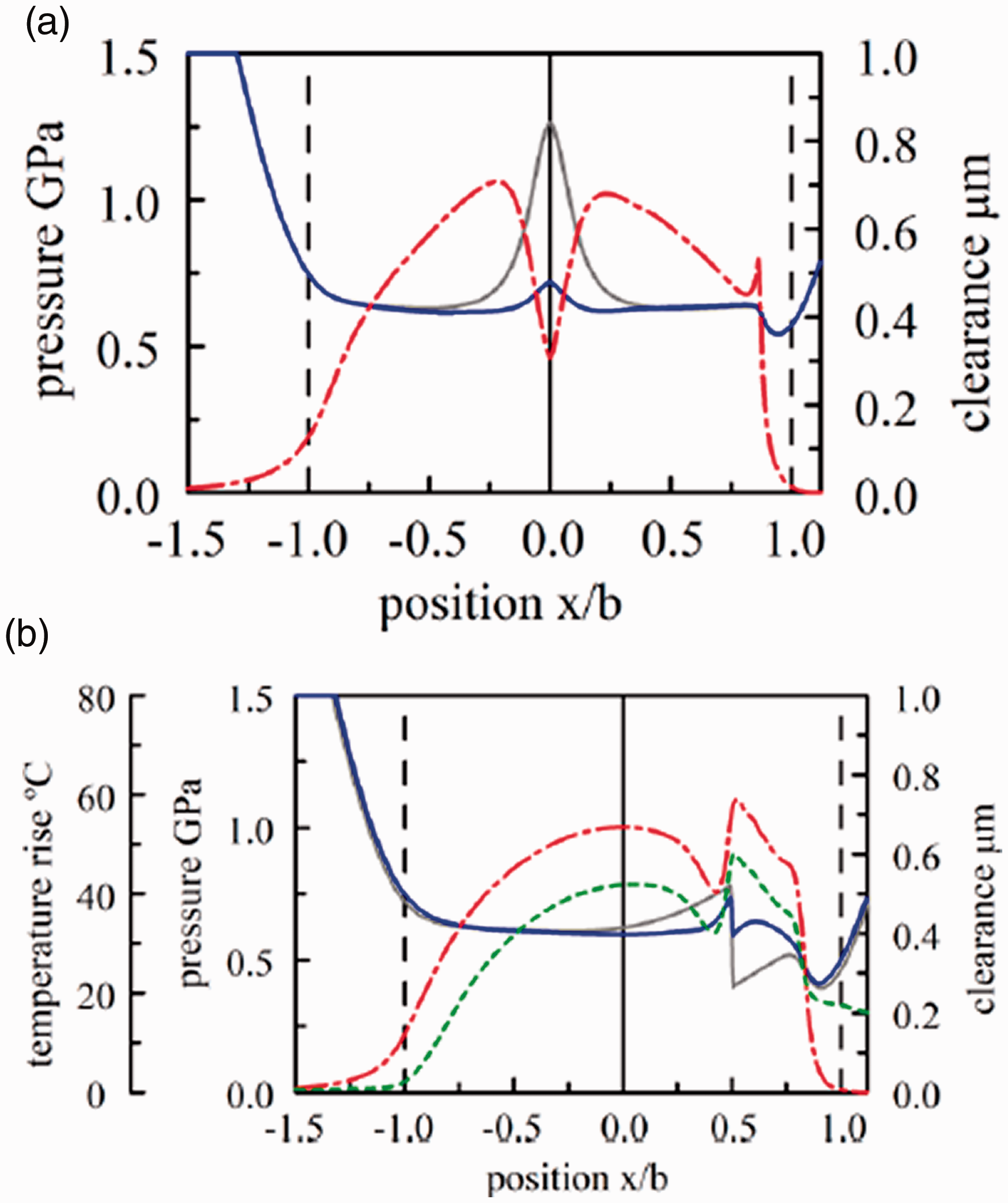
The above analysis was used to determine the behaviour of a cylindrical void in a rolling contact and that of a crack in a sliding conjunction and the results are shown in Figure 8(a) and (b).

Figure 8.

(a) Rolling contact, cylindrical void, r/b = 0.1, defect depth 1.5r. Defect at x = 0. Full line – clearance, chained – pressure, dashed – temperature, grey – distortion produced by smooth pressures; (b) sliding contact, vertical crack, depth 0.7b. Crack at x/b = 0.5.

The results are shown for one instant of time. For the cylindrical void there is a significant local reduction in pressure and, because of this, the increase in clearance is substantially reduced from the initial roughness found using the smooth EHL pressures.

Similarly, the crack generates significant pressures around it with, for the crack location shown, a drop to the left of the crack and a large increase to the right. These pressures significantly modify the initial profile.

Inclusion of the K_dp_d term

The results shown in Figure 8(a) and (b) ignore the effect of the perturbation pressures on the defect, the ${\mathrm{K}}_{\mathrm{d}}{\mathrm{p}}_{\mathrm{d}}$ term of equation (8). However, with p_d obtained this term may be included and the analysis repeated. Since this will modify the value of p_d it may be necessary to repeat the process two or three times. For stability and efficiency it is useful to use an under-relaxation factor.

The final behaviours obtained are shown in Figure 9(a) and (b) which replicate the conditions of Figure 8. With the cylindrical void the amplitude of the surface deformation is reduced and the pressure perturbation is approximately halved.

Figure 9.

(a) As Figure 8(a) with ${\mathrm{K}}_{\mathrm{d}}{\mathrm{p}}_{\mathrm{d}}$ included; (b) as Figure 8(b) with ${\mathrm{K}}_{\mathrm{d}}{\mathrm{p}}_{\mathrm{d}}$ included.

The effect on the crack is similarly significant with the pressure perturbations being reduced. However, most significant is the reduction in the relative displacements of the two sides of the crack with this being more than halved.

In interpreting the results of Figures 8 and 9(a) it should be noted that the elastic behaviours differ. In Figure 8(a) and (b) the deformation (the difference between the roughness and the clearance) is produced by the pressures acting on a half space with the defect absent. In Figure 9(a) and (b) the defect is present and a smaller pressure variation is needed to generate the same displacements.

Changes in K_d

In the above it has been assumed that the flexibility perturbation remains unchanged as the defect moves through the conjunction. However, there are a limited number of occasions where it will vary. For example, an inclined crack may open in front of the contact but close as it passes under it. The flexibility perturbation will thus change part way through the conjunction. Since the calculation of the roughness, r, in equation 10 simply requires that deformation be defined as a function of the defect location, incorporation of these changes is straightforward.

Accuracy

In order to check the accuracy of the analysis the results were compared with results presented in Quinonez and Morales-Espejel. ¹⁵ These appear to be the only available results for non-stationary defects under both rolling and sliding conditions. The conditions examined in Quinonez and Morales-Espejel ¹⁵ are somewhat artificial and considered transverse, cylindrical inclusions in one surface. The mating surface was assumed rigid. Thermal effects were ignored as were shear rate effects and a Roelands' viscosity-pressure relationship was adopted.

These conditions were replicated and the results from the current analysis compared with those in Quinonez and Morales-Espejel. ¹⁵ Two typical results are shown in Figure 10(a) and (b).

Figure 10.

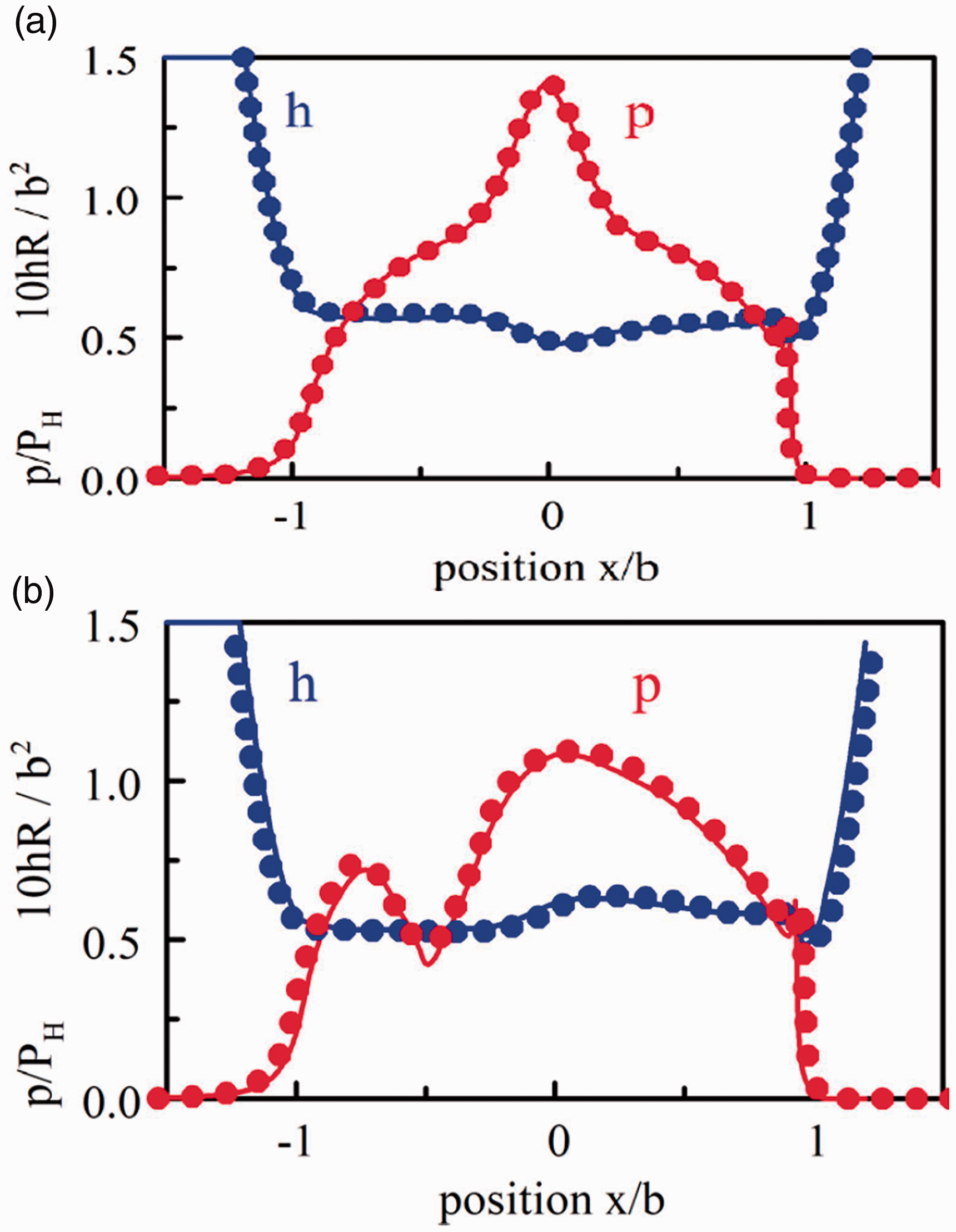
(a) Comparison of current analysis with Quinonez and Morales-Espeje. ¹⁵ Pure rolling, cylindrical defect of r/b = 0.2, depth 1.5r, with a modulus four times that of the surrounding material. Defect at x = 0. (b) Sliding, SRR = 1, cylindrical defect of r/b = 0.2, depth 1.5r, with a modulus 0.25 times that of the surrounding material. Defect at x/b = –0.25. Full lines – current analysis; dots – results from Quinonez and Morales-Espeje. ¹⁵

In both cases the agreement is adequate, suggesting that the current, rapid approach can yield accurate results. In Figure 10(b) sliding eliminates any significant variation of clearance over the defect (there is a small variation produced by the interaction of the pressure and fluid compressibility) and the variation in clearance on the right hand side of the conjunction is that produced in the inlet and transported at the mean surface speed.

Calculation times

For the examples given above, calculation of the flexibility perturbation matrices took around 15 s; evaluation of the sinusoidal behaviour around 5 min for two dimensional problems and around 1 h for three dimensional. Combining these to find the perturbed behaviour occupied, typically, less than 2 s for the first approximation and under 3 s for the result including the ${\mathrm{K}}_{\mathrm{d}}{\mathrm{p}}_{\mathrm{d}}$ term. These values are for two-dimensional problems and increase somewhat for three dimensions (exact comparison is difficult because a coarser FE mesh was used for the 3D examples). All calculations were for a standard PC.

Results

The aim of the present paper is to outline an extension of the perturbation analysis to allow the analysis of EHL contacts with surface and sub-surface defects.

The behaviour varies with both the nature of the EHL contact and with the type of defect and it is impossible to provide a full account of all possible effects. Accordingly, only a limited number of examples will be given. However, all results presented include the ${\mathrm{K}}_{\mathrm{d}}{\mathrm{p}}_{\mathrm{d}}$ term.

Cylindrical inclusion

Figure 11 shows the pressures, clearances and sub-surface stresses as a transverse cylindrical inclusion with a modulus three times that of the bulk material passes under the contact.

Figure 11.

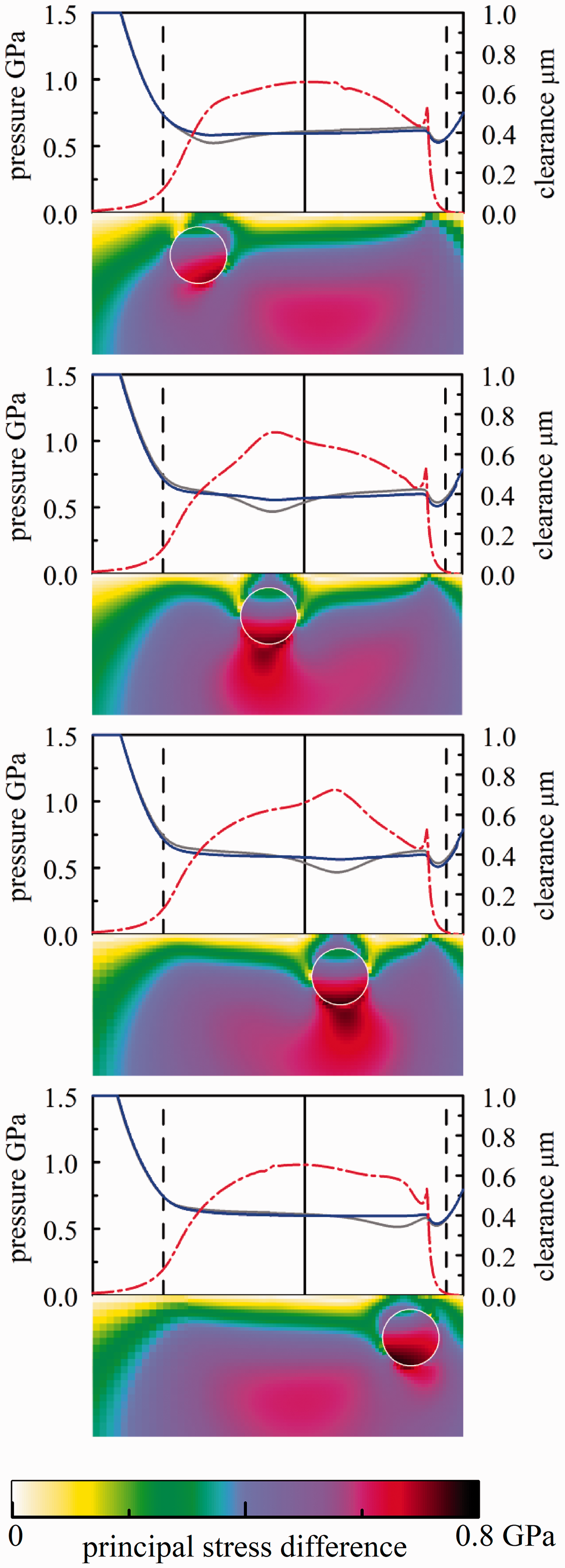
Pressure, clearance and stresses for a cylindrical inclusion. r/b = 0.2, defect depth = 1.5r. Rolling contact, inclusion modulus = three times that of the bulk material.

The action of the smooth pressures on the inclusion tends to produce a local reduction in clearance above it. However, hydrodynamic action largely eliminates this but produces a local increase in pressure. The inclusion generates a substantial increase in the maximum principal stress difference in the surface material around the bottom of the defect. This appears to be due to the higher stiffness of the defect reducing the horizontal strain locally while affecting the vertical stress to a lesser extent. The increase as the defect passes the centre of the conjunction is from about 0.55 GPa without the inclusion to around 0.75 GPa when it is present. A converse affect occurs for the stresses inside the defect and the largest magnitude appears to occur near its base with a value of about 0.78 GPa. These stresses max be compared with the maximum value for a Hertz contact of 0.6 GPa at a depth of 0.78b.

Spherical void

Figure 12 shows the effect of a small spherical void under a sliding EHL contact. The values are symmetrical about y and, for clarity, only half the region is shown. Also, for clarity, the clearances are shown inverted, Results are shown as the defect passes the centre of the conjunction. The smooth pressures produce a local increase in clearance from 0.4 µm to about 0.5 µm. This is very largely flattened by the hydrodynamic action, with a local reduction in pressure from 1 GPa to around 0.7 GPa.

Figure 12.

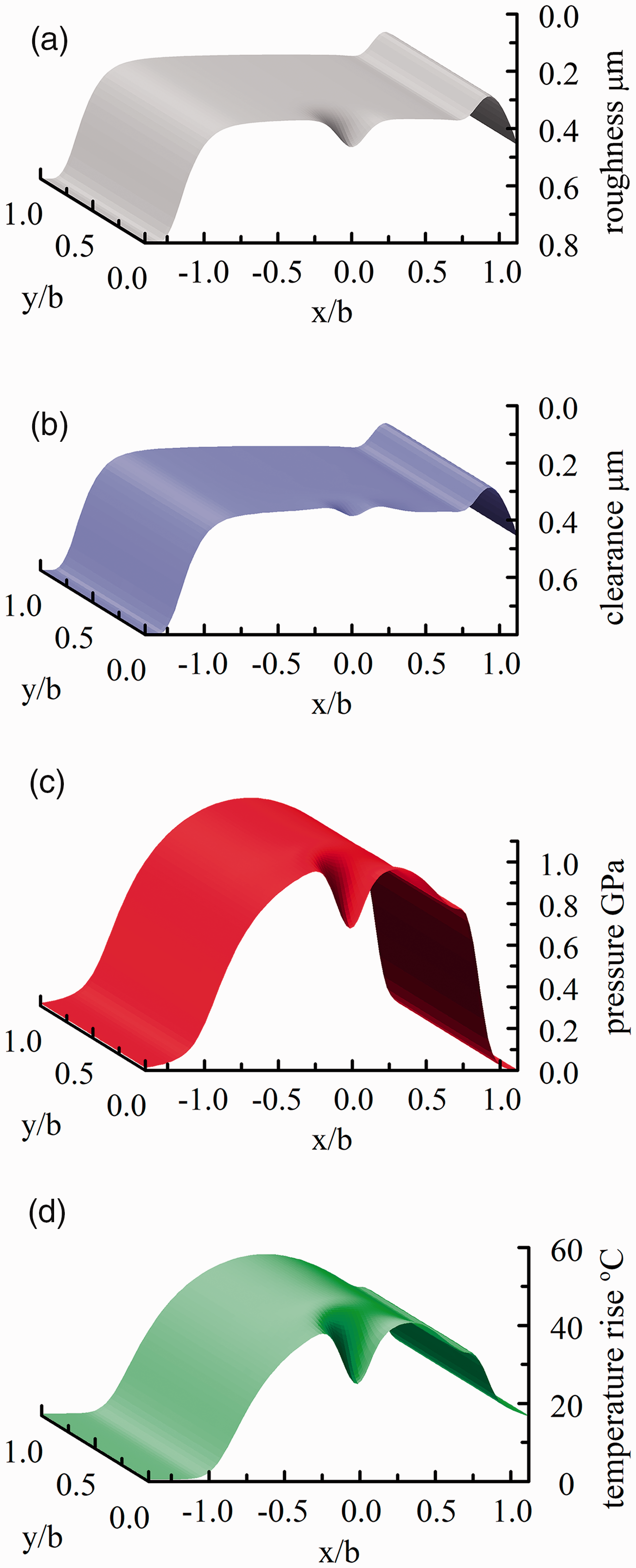
Behaviour of a spherical void, r/b = 0.1, defect depth = 1.5r, in a sliding EHL contact as it passes the centre of the conjunction. Profile generated by smooth pressures, clearances, pressures, temperature rise at the film centre. The behaviour is symmetrical about the y axis.

As is typical in sliding EHL contacts the temperature and pressure are closely linked and there is a local reduction in temperature rise from over 40 to about 25 °C.

Vertical crack

Figure 13 shows the behaviour of a vertical crack in a sliding contact. The smooth pressures produce a step increase in clearance across the crack when it is on the inlet side of the conjunction. This changes to a step decrease on the exit side. Hydrodynamic action produces a local drop in pressure across the crack on the inlet side; a local drop on the exit. This tends to reduce the clearance variation. However, the behaviour is complicated by the tendency of the pressure and clearance variations to propagate at the mean surface velocity. This is clearly visible in the graphs with the crack located at –0.25 b and 0.25 b.

Figure 13.

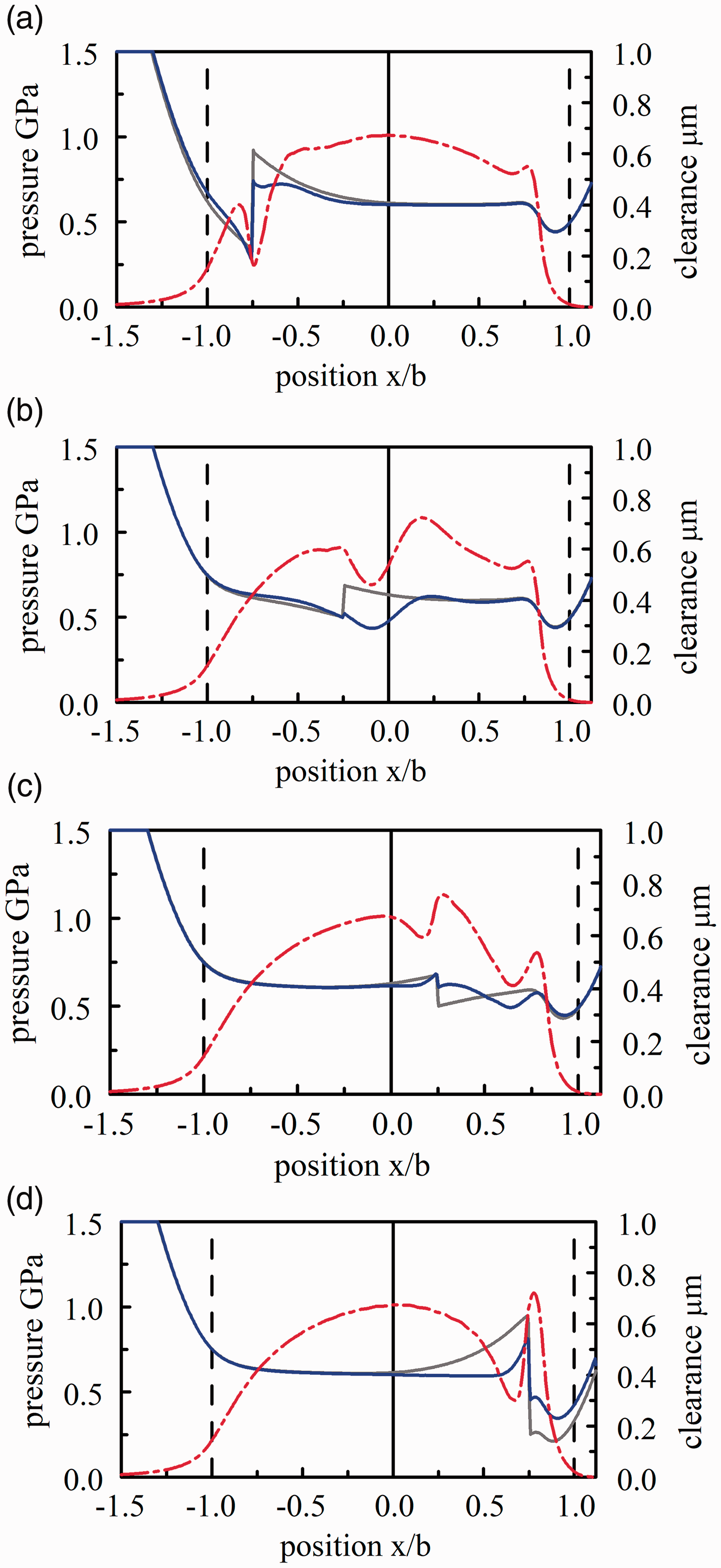
Behaviour of a vertical crack, d/b = 0.7. Sliding contact. For clarity, the temperature rises have been omitted.

As with the cylindrical inclusion it is possible to determine the stress distributions in the surface. However, with cracks it is the stress intensity factor at the crack tip that is of interest and this can be estimated from the local stress field. Because a vertical, frictionless, sliding crack in which the faces remain in contact has been considered only the mode 2 stress intensity factor, K_II, is relevant and this has been estimated as the crack passes through the conjunction. Results are shown in Figure 14 for a range of crack depths.

Figure 14.

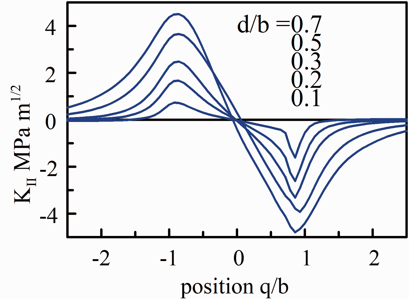
Stress intensity factor K_II for a vertical crack under sliding conditions for a range of crack depths.

Repetition of the analysis for a rolling contact showed very little change in the stress intensity factors although the pressure perturbations were significantly greater immediately adjacent to the crack. It was also noted that use of the smooth EHL pressures produced very similar factors.

Although further work using different crack geometries and different operating conditions is required, the results suggest that the smooth EHL pressure distribution might be used to obtain reasonably accurate estimates of the stress intensity factors.

Effect of defect depth

For inclusions lying well below the surface, stresses calculated using the smooth EHL pressures are adequate. Nearer the surface a full EHL analysis is required. In an attempt to provide some information about this, a range of transverse cylindrical and elliptical cavities was examined. These covered a range of depths and defect sizes and the results are summarised in Figure 15.

Figure 15.

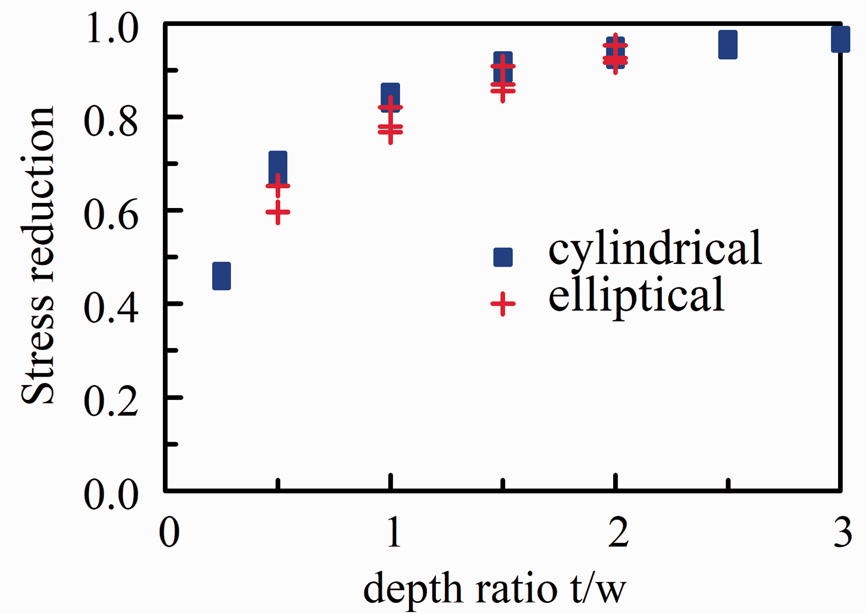
Effect of defect depth for cylindrical and elliptic transverse cavities. The elliptical defects all had a width to height ratio of 2. Results are for defect heights of 0.1, 0.2 and 0.5b. Stress reduction is the ratio of the maximum principal stress difference to that calculated using the smooth EHL pressures.

All results are for a rolling contact and are for the moment that the cavity passes the contact centre. Although there is some scatter, the broad trend is clear. Where the depth, t, of the material above the defect is greater than twice the defect’s width, w, the error introduced by using the smooth EHL pressures is below 10%. As the material thickness decreases the error steadily increases, It should, however, be noted that the curve only applies to the two defects examined and there was, for example, a far smaller difference in the stresses with an elliptical defect having a height twice its width.

In spite the limited range of examples shown, it is hoped that the results give some indication of when a full EHL analysis may be required and when a simplified stress calculation will suffice.

Conclusions

A method for the rapid analysis of EHL contacts with surface and sub-surface defects has been presented and some examples given. The analysis contains three distinct stages. First the effect of the defect on the elastic behaviour of the surface is considered. It is shown that the relationship between surface pressure and displacement can be simplified to that of half spaces plus a correction local to the defect. This correction moves with the defect. Second, the response of an EHL contact to sinusoidal variations in clearance is required. These variations vary both with position and time. Finally the two are combined using Fourier methods to obtain the system response.

This process separates the elastic and EHL analyses so, for example, the EHL analysis needs to be carried out only once for any given operating conditions and the results will apply to all defect geometries. Similarly, the elastic analysis will be valid for any operating conditions and will cover all geometrically similar defects.

The analysis applies only to line contacts although the defects may be three dimensional. However, the error involved in using it for other contacts such as the ball on a plane that is widely used in EHL experiments should be small provided the radius of the line contact is adjusted so the Hertz widths and pressures match.

Analyses of a number of geometrically simple defects suggests that, although the smooth EHL pressures typically produce large surface deformations, these deformations are largely eliminated by hydrodynamic action. However, substantial pressure changes may be generated above the defect and these significantly alter the stress distributions.

Where the depth of the defect is large it has little effect on the surface deformations and there is no need for a full EHL analysis. Here it is sufficient to use the smooth EHL pressures to estimate the stresses. The depth above which a full EHL analysis is required is somewhat uncertain but on the basis of a limit number of calculations it is suggested that provided the thickness of material above the defect is greater than twice the defect size (defined as its maximum dimension) the error introduced should be below 10%.

Similarly, analysis of a vertical crack suggests that adequate estimates of the stress intensity factors might be obtained using the smooth pressure distributions. This needs further investigation but would avoid the need for any full EHL analyses.