Sage Journals: Discover world-class research

Abstract

A robust algorithm for solving the Bancroft version of the Pochhammer–Chree (PC) equation is developed based on the iterative root-finding process. The formulated solver not only obtains the conventional n-series solutions but also derives a new series of solutions, named m-series solutions. The n-series solutions are located on the PC function surface that relatively gradually varies in the vicinity of the roots, whereas the m-series solutions are located between two PC function surfaces with (nearly) positive and negative infinity values. The proposed solver obtains a series of sound speeds at exactly the frequencies necessary for dispersion correction, and the derived solutions are accurate to the ninth decimal place. The solver is capable of solving the PC equation up to n = 20 and m = 20 in the ranges of Poisson’s ratio (ν) of 0.02 $\leq$ ν $\leq$ 0.48, normalised frequency (F) of F $\leq$ 30, and normalised sound speed (C) of C $\leq$ 300. The developed algorithm was implemented in MATLAB®, which is available in the Supplemental Material (accessible online).

Keywords

Vibration and acoustics wave equation of motion frequency equation sound speed group velocity bisection method

Introduction

The Hopkinson bar (HB)^1–4 has been traditionally used to measure dynamic transient loads at the near field of high-energy sources. Currently, the HB is also used as a stress transducer for the non-destructive assessment of materials and structures.⁵ In contrast, the split Hopkinson bar (SHB)^6–16 has been widely used to measure the uniaxial stress–strain and strain rate–strain curves of versatile materials at strain rates of approximately 10²–10⁴ s⁻¹.

In both the HB and SHB, a transient elastic wave travels the bar. The detailed profiles of the wave, i.e., the rise time and mode of fluctuation in the plateau region, vary with travel. Therefore, the elastic wave profiles in the HB and SHB must be predicted at an axial position of interest from the measured profile (at a different point); this is called dispersion correction.^9,17–24 The distortion of the elastic wave shape with travel mainly results from the fact that a high-frequency wave component that constitutes the overall wave is sluggish compared to a low-frequency component. Therefore, in standard dispersion correction, the phases of a series of wave components (with different frequencies) are corrected at a given axial position. In the literature,^25–28 the measured magnitude of the travelling wave is also corrected because the wave magnitude depends on the axial position (i.e., phase) and radial position in the bar.

To perform standard dispersion correction and magnitude correction of the measured elastic wave in the HB and SHB, the sound speeds of a series of elastic waves with different frequencies must be known a priori for a given bar. The necessary sound speed values can be obtained for a range of frequencies by solving the Pochhammer–Chree (PC) equation.^29–32

According to Love,²⁹ Pochhammer (1876)³⁰ and Chree (1886, 1889)^31,32 independently derived the wave equation of motion (vibration equation) for an infinite, isotropic, and elastic bar. The PC equation is valid for a cylinder with finite length if the radius is small compared with the wavelength.²⁹ Its solution is the relation between c and Λ (see the nomenclature in the Supplemental Material (Section 1) for the notations used herein). This c–Λ relation can be used to obtain the frequency via the equation c = fΛ. While the solutions to the PC equation were sought via various methods, most studies that solved the PC equation for dispersion correction used the root-finding process based on iterative techniques.^{4,23,24,40–43} This study also employs iterative techniques for root-finding. The challenges in solving the PC equation and the resultant state-of-the-art PC equation solutions are described in the Supplementary Material (Sections 2.1 and 2.2, respectively).

Despite the difficulty of solving the PC equation, obtaining a detailed algorithm to solve the PC equation is challenging. Moreover, the studies reporting the solutions did not reveal the details of their numerical schemes.^4,23,24 Because of the cumbersome nature of handling the PC equation to obtain the necessary c–f relation for a specific bar, only a few studies involving dispersion correction^4,24,25 have recently solved the PC equation. In the foregoing references,^4,23,24 solutions for some considered Poisson's ratios (0.2, 0.287, 0.3, and 0.35) were obtained based on in-house schemes (the details are undisclosed) and were provided in graphical form within limited ranges of frequencies and sound speeds.

The objective of this study is to provide an open-source solver of the PC equation based on a robust algorithm for the following reasons. First, there were no open-source solvers widely used; since the introduction of the PC equation in 1876, the availability of an open-source solver with proven reliability is long overdue. Such an open-source solver will afford researchers with a verifiable tool for solving the PC equation, which will facilitate dispersion correction of measured elastic waves in a (split) Hopkinson bar. It will also encourage program development and formulation of candidate algorithms.

Second, most studies that provided graphical or tabular solutions^{4,23,24,33–45} (without the detailed solution process) reported sound speeds at a constant a/L interval or at an arbitrary f interval. Therefore, the solution frequencies were unnecessary frequencies for the dispersion correction of the user that necessitated the interpolation of the solutions at the required frequencies. Some examples of the required constant frequency intervals for dispersion correction are summarised in Table 1. Accordingly, this study aims to formulate a solver that yields solutions exactly at the frequencies necessary for dispersion correction.

Table 1.

F_{dc_max} and dF_dc for a range of a values when T_o = 200 µs, dt = 0.2 µs, and c_o = 5000 m/s (N_y = f_Ny/df_dc = F_{dc_max}/dF_dc = 500).

Bar radius (mm)	5	7.5	10	12.5	15	20	35	50
$F_{dc_\max} = a f_{Ny} / c_{o}$	2.5	3.75	5.0	6.25	7.5	10.0	17.5	25.0
$d F_{dc} = a {d f}_{dc} / c_{o}$	0.005	0.0075	0.01	0.0125	0.015	0.02	0.035	0.05

Third, most studies that afforded graphical or tabular solutions^{4,23,24,33–45} (without the solution process) derived the solutions in limited ranges of approximately 0 ≤ c/c_o ≤ 2 and 0 ≤ a/Λ ≤ 2 up to n = 4 (corresponding to the range 0 ≤ af/c_o ≤ 4). The studies that only afforded graphical or tabular solutions^{4,23,24,33–45} (without the solution process) were also performed in similar ranges. As summarised in Table 1, wider ranges of frequencies (and sound speeds) are necessary for dispersion correction. The solutions should also be derived up to higher orders for a wider range of Poisson’s ratios than those derived in existing studies.^{4,23,24,33–45} However, studies that determined solutions across wide ranges of frequency, sound speed, order, and Poisson’s ratio are rare. Therefore, this study aims to provide a solver that yields solutions across wider ranges of the foregoing quantities simultaneously (0.02 $\leq$ ν $\leq$ 0.48, 1 $\leq$ order $\leq$ 20, af/c_o $\leq$ 30, and c/c_o $\leq$ 500).

Finally, as described in the Supplemental Material (Section 3), the PC equation derived by Bancroft³⁵ is advantageous over other versions in developing a solver in that the normalized solutions (af/c_o vs. c/c_o) can be derived by inputting only one variable (Poisson's ratio) that describes medium characteristics. However, it is difficult to find the solvers that exploited such an advantage explicitly. Accordingly, this research aims to provide a solver that exploits such an advantage of the Bancroft version.

Pochhammer–Chree equation

Among the many versions of the PC equation, those introduced by Love,²⁹ Redwood,⁴⁴ and Bancroft³⁵ are introduced in the Supplemental Material (Sections 3.1–3.3) with an emphasis on the benefit of the Bancroft version in the solution process and post-processing stage. To aid in comprehending the dependent nature of the PC function on frequency, sound speed, and wavelength (which eventually aids in developing the scheme for solving the equation), this study expresses the Bancroft version using physics-friendly non-dimensional variables, instead of x, $γ a$ , and β, used in the original paper.³⁵

The physics-friendly non-dimensional variables employed herein are C (=c/c_o), L (=a/Λ), and F (=af/c_o), regarded as normalised sound speed, wavelength, and frequency, respectively. According to c = fΛ, the relation between F, C, and L is given by F = CL. This relation is illustrated in the Supplemental Material (Section 3.4). In terms of F and C, the Bancroft version of the PC equation is expressed as (see Section 3.4 of the Supplemental Material)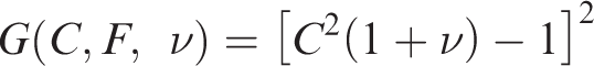

G (C, F, ν) = {[C^{2} (1 + ν) - 1]}^{2}

Φ [2 π \sqrt{β F^{2} (1 + ν) - {(F / C)}^{2}}] - [β C^{2} (1 + ν) - 1] \times \{C^{2} (1 + ν) - Φ [2 π \sqrt{2 F^{2} (1 + ν) - {(F / C)}^{2}}]\} = 0

(1)

If an F value is considered as the independent variable, the resultant C value that satisfies equation (1) can be obtained under a fixed value of ν. Once the C (=c/c_o) vs. F (=af/c_o) relation is obtained, the c–f relation necessary for dispersion correction can be obtained in the post-processing stage by using the information on the medium, i.e., c_o and a values. This study solves equation (1).

Solution process

Backgrounds: F_max and dF_dc

As a background for the PC equation solution process, reviewing the necessary values of maximum F (F_dc__max) and F interval (dF_dc) in a typical dispersion correction of elastic waves in the (split) Hopkinson bar may be informative. Consider a linearly elastic wave travelling along the axial direction of a circular bar with a radius (a) of 10 mm and a thin-bar sound speed (c_o) of 5000 m/s (c_o = $\sqrt{E / ρ}$ ). Suppose the elastic wave is measured at a time interval (dt) of 0.2 µs and a time window (T_o) of 200 µs is considered. Then, the sampling frequency (f_s = 1/dt) is 5 MHz; the number of time data (N = T_o/dt) is 1000; the frequency interval (df_dc = f_s/N) for dispersion correction is 5 kHz; the dF_dc (= adf_dc/c_o) value is 0.01, the Nyquist frequency (f_Ny = f_s/2) is 2.5 MHz, and the maximum F value (F_{dc_max} = af_Ny/c_o) for dispersion correction is 5.0. The number of frequencies in dispersion correction (N_y; Nyquist number) is N_y = f_Ny/df_dc = F_{dc_max}/dF_dc = 500.

The F_{dc_max} and dF_dc values calculated using the above approach are listed in Table 1 for a range of a values in the case where T_o = 200 µs, dt = 0.2 µs, and c_o = 5000 m/s. The list indicates that if the bar radius is increased to 50 mm, an F_{dc_max} value as high as 25 is required under the considered condition. This study aims to solve an F_{dc_max} value of up to 30. The table further indicates that the frequency interval necessary for dispersion correction, dF_dc, increases in proportion to the bar radius. According to the procedure described in the preceding paragraph, an increase in dt by x times results in 1/x times the value of F_{dc_max}; increasing the time window (T_o) by x times yields 1/x times the value of dF_dc. A review paper on the dispersion correction of elastic waves in the (split) Hopkinson bar will be published elsewhere.

Scheme

The shapes of the PC function curves in two dimension and PC function surfaces in three dimension are illustrated in the Supplemental Material (Sections 4.1 and 4.2). This study derives the conventionally known n-series solutions which are located on the PC function surface that relatively gradually vary in the vicinity of the roots. It further obtains new-type solutions, named m-series solutions, located between two PC function surfaces with (nearly) positive and negative infinity values (see Section 4.1 of the Supplemental Material).

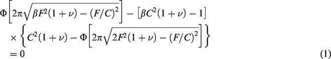
Based on the illustrated function shapes in the Supplemental Material, a schematic of the dispersion curve (with n $\geq$ 2 and m $\geq$ 1) in the C–F domain is shown in Figure 1. In this figure, the index (subscript) of F increases, starting from one, as the F value decreases from F_max (= F₁). In the regime where the F value is relatively high, routine X is implemented; in this routine, the F value is independently varied to obtain the root of C. When the slope of the dispersion curve increases towards infinity with a decrease in F, routine Y is implemented. In this routine, the C value is independently varied to obtain the root of F.

Figure 1.

Algorithm (bisection method combined with linear extrapolation) employed in routines X (X_a and X_b) and Y for solving the PC equation for n $\geq$ 2 and m $\geq$ 1.

In this research, the orders of dispersion curves are counted at intermediate F values: F_start(1) and F_start(2). The pre-processing details for determining F_start(1) and F_start(2) and the routine for counting the order are described in the Supplemental Material (Sections 5.1 and 5.2). Once the orders are determined, routines X_a and X_b are implemented. In routine X_a, the search for the root proceeds by increasing F starting from F_start(1) and F_start(2), whereas in routine X_b, the program searches for the root by decreasing F starting from F_start(1) and F_start(2).

The algorithm of routine X is explained here using the case of routine X_b. The roots, C_i-2 and C_i-1, in the two previous frequencies (F_i-2 and F_i-1, respectively) are linearly extrapolated to obtain the approximate solution, C_a, at the current frequency, F_i. This is followed by obtaining the numerical solution C_i at F_i by the bisection method.

In the low F regime (Figure 1), where the dispersion curve increases extremely rapidly towards infinity with the decrease in F (routine Y), considering C as the independent variable and obtaining the resultant value of F at each C value is convenient. In this regime (routine Y), the F values (F_j-2 and F_j-1) in the two previous sound speeds (C_j-2 and C_j-2, respectively) are linearly extrapolated to obtain the approximate solution, F_a, at the current sound speed, C_j. This is followed by obtaining the numerical solution, F_j, at C_j by the bisection method; the C values are varied independently (C-driven process) to obtain the F values. Detailed algorithms for manifesting routines X (X_a and X_b) and Y are described in the Supplemental Material (Sections 5.3–5.5).

After routines X_a, X_b, and Y are completed, the F values in each routine are merged to form a single matrix; this is also the case for the C values in these three routines. Subsequently, for each order, the (F, C) dataset for plotting the obtained solution (the C–F plot) is prepared. The obtained solutions (both n- and m- series) for a range of Poisson’s ratios are presented in the Solutions of PC equation section.

The C_g (normalised group velocity) vs. F plots are prepared in the post-processing stage using the obtained (C, F) dataset. The definition of C_g in the C–F domain and the method of obtaining it are available in the Supplemental Material (Section 5.6).

If the solution itself is required for the purpose of plotting the C vs. F diagram, the (F, C) dataset is then sufficient. Furthermore, the C vs. F diagram can be prepared via a graphical method.⁴⁵ As mentioned, for the purpose of dispersion correction, the exact C_dc values at exactly necessary F_dc values must be obtained, while the (F, C) dataset generally differs from the (F_dc, C_dc) dataset. The (F_dc, C_dc) dataset is obtained herein via linear interpolation of the (F, C) set, followed by the application of the bisection method (see Section 5.7 of the Supplemental Material).

Results and discussion

Solver verification

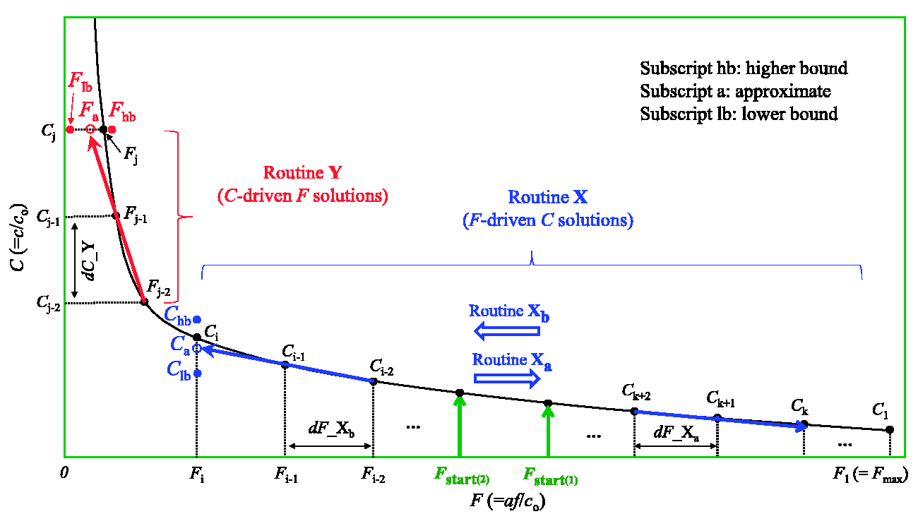
The proposed solver was verified first using tabular solutions available in the literature. Figure 2(a) plots the n = 1 solutions available in Bancroft’s study (Table I in³⁵) at varying Poisson’s ratios. In Ref. 35, the solutions in the C–L domain were listed at L intervals of 0.025 or 0.1. Accordingly, this study transformed the tabulated L values to F values in order to obtain the C–F domain solutions; the results are presented in Figure 2(a) as open circles. In this figure, the intervals in Bancroft’s data are irregular in the F axis owing to the transformation from L to F. The figure also shows the solutions obtained using the proposed solver at a constant F interval (dF) value of 0.05 (marked as “×”); the C solutions at a regular F interval are necessary for dispersion correction.

Figure 2.

(a) Comparison of n = 1 solutions of Bancroft³⁵ with those of present study (dF = 0.05) at different Poisson’s ratios; (b) comparison of n = 2 and n = 3 solutions of Davies³⁶ with this study (dF = 0.05) at a Poisson’s ratio of 0.29.

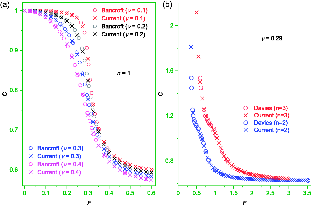
Figure 2(b) plots the n = 2 and n = 3 solutions available in Davies’s study (Table 11 $\cdot$ 1 in³⁶) at a Poisson’s ratio of 0.29. Davies's study also obtained the solutions in the C–L domain. The L values of the tabulated data were transformed to F values, which yielded irregular F intervals in the C–F domain. The results are presented in Figure 2(b) as open circles. The figure also shows the solutions obtained herein at a constant dF value of 0.05 (marked as “×”).

As shown in Figure 2, reasonable consistency is observed between the results reported in the literature (open circles) and those herein (marked as “×”), indicating the reliability of the solutions obtained in this research. In the studies of Bancroft and Davies, solutions (the C value at a given L) are available down to fifth and third (or fourth) decimal places, respectively. In the proposed solver, the tolerance limit (error) in the bisection algorithm is set as 10⁻¹⁰; the solutions obtained herein are accurate down to the ninth decimal place.

Solutions of PC equation

The proposed solver yielded n-series solutions over a range of Poisson’s ratios up to n = 20. The results presented in Figure 3 are for an F value of up to 10 and a C value of 2 or 3; the insets plot the curves in wider ranges. Figure 3 shows points around which the given dispersion curve abruptly changes; herein, these points are referred to as abrupt-change points (ACPs). At a given Poisson’s ratio (Figure 3(a)), the distance between two ACPs in adjacent curves decreases as the order (n) increases. At higher orders, this distance becomes extremely small such that the adjacent curves seem to be connected, but a magnified view (not shown) verifies that they are not. An overly close ACP distance causes a deviation of the curve-tracking process; nearby curves are falsely tracked around the ACPs. Accordingly, more refined dC and dF values are necessary around the ACPs to keep track of higher-order dispersion curves, especially at a small Poisson’s ratio; however, this increases the computational burden. The proposed solver considers the positions of the ACPs in the C–F domain while setting up the dC and dF values for tracking the dispersion curves.

Figure 3.

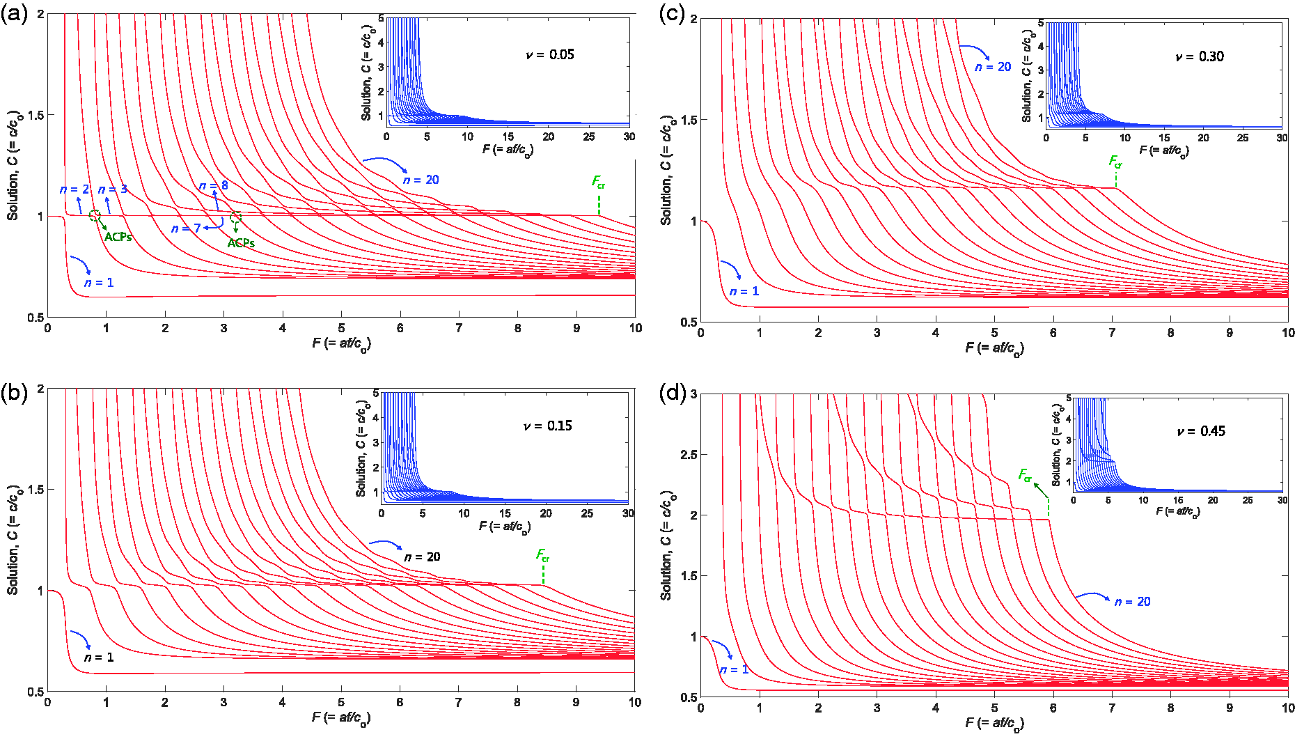
‘n-series’ solutions at Poisson’s ratios of (a) 0.05, (b) 0.15, (c) 0.30 and (d) 0.45; F_cr is explained in Supplemental Material (Section 6.1).

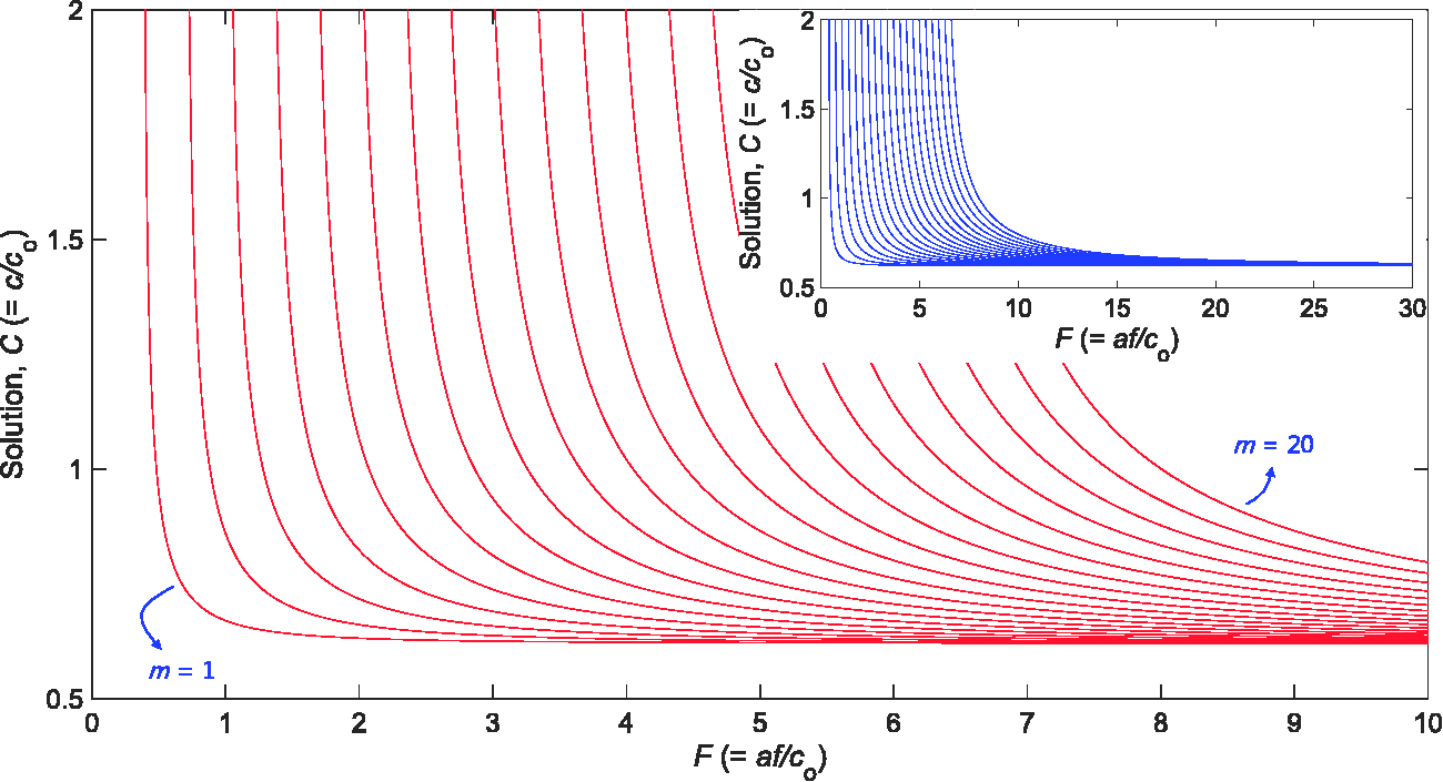
The proposed solver also yielded m-series solutions up to an order of 20 for a Poisson’s ratio of 0.3 (Figure 4). The curves for other Poisson’s ratios (0.05 $\leq ν \leq$ 0.45) are available in the Supplemental Material (Section 6.2). The presence of the second group of m-series curves is also discussed in the Supplemental Material (Section 6.3).

Figure 4.

‘m-series’ solutions at a Poisson’s ratio of 0.30.

The proposed solver obtains the C_g vs. F plot using the matrices of C and F (Figures 3 and 4). The results (C_g vs. F plots) for n-series and m-series solutions at a Poisson’s ratio of 0.3 are available in the Supplemental Material (Sections 6.4 and 6.5) up to order 20.

The solver finally calculates the F_dc and C_dc values by using the (C, F) dataset. The results (C_dc vs. F_dc plots) for n-series and m-series solutions at a Poisson’s ratio of 0.3 (dF_dc = 0.02) are presented in the Supplemental Material (Section 6.6) up to order 20. The proposed program writes the (C_dc, F_dc) dataset of each order to an Excel® file (Cdc-Fdc.xlsx).

Overall discussion

The proposed solver does not request the user to input any bar information other than the Poisson’s ratio. Once the C_dc vs. F_dc dataset (non-dimensional quantities) at a given ν is derived using the solver, in the second step, the c_dc vs. f_dc set (dimensional quantities) necessary for dispersion correction is obtained by the user using further specific information on considered bar (c_o and a). Therefore, only the influence of Poisson's ratio on dispersion curve shapes needs to be considered in developing a solver when the two-step approach is employed. On the other hand, in the one-step approach^[40–43], the c vs. f set (or c vs. Λ set) is directly solved under fixed medium variables (ν, a, and c_o in the Bancroft version; a, ρ, λ, and µ (or a, ν, ρ, and Ε) in Love and other versions); the solver requests to input the foregoing variable values. Therefore, the influences of these three or four medium variables on dispersion curve shapes must be considered in developing a solver if the one-step approach is to be employed. In this regard, the two-step approach based on the Bancroft version has an advantage in developing a robust PC equation solver.

The values of user variables such as dC and dF are pre-set in the proposed program. These values reflect the characteristics of the complicated shape of the PC function. The validity of the pre-set user variable values in tracking the dispersion curves was checked up to the order of 20 (for both n- and m-series) for a wide range of Poisson’s ratios (0.02 $\leq$ ν $\leq$ 0.48) at intervals of 0.001. The proposed solver with the pre-set user variable values is capable of solving the PC equation in the ranges of F $\leq$ 30 and C $\leq$ 500. The pre-set values of all user variables in this study may be subject to modifications for orders higher than 20 or under unverified Poisson's ratio conditions (if the order is ≤20) for the steady tracking of dispersion curves. In such a case, the curve of interest of a particular order can be tracked again after modifying the user variable values such as dC and dF specific to the curve (see Section 7 of the Supplemental Material).

Conclusion

A robust algorithm for solving the Bancroft version of the PC equation was developed based on an iterative root-finding process that refers to the illustrated function shape and combines the bisection, linear extrapolation, and linear interpolation methods. The developed algorithm was implemented in MATLAB®; it is available in the Supplemental Material accessible online.

The proposed solver not only obtains the conventionally known n-series solutions but also a new series of solutions, named m-series. Whereas the n-series solutions are located on the PC function surfaces that vary relatively gradually in the proximity of the roots, the m-series solutions are located between two PC function surfaces with nearly positive and negative infinity values. The solver derives a series of sound speeds exactly at the necessary frequencies for dispersion correction and yields solutions that are accurate to the ninth decimal place. Furthermore, it is capable of solving the PC equation up to n = 20 and m = 20 in the Poisson’s ratio range of 0.02 $\leq$ ν $\leq$ 0.48, F $\leq$ 30, and C $\leq$ 500.

The validity of the pre-set user variable (e.g., dC and dF) values in the proposed solver in tracking the dispersion curves was verified up to the order of 20 (for both n- and m-series) in a wide range of Poisson’s ratios (0.02 $\leq$ ν $\leq$ 0.48) at intervals of 0.001. For unchecked Poisson’s ratios (if any), the curve of interest of a particular order can be tracked again after modifying the user variable values such as dC and dF specific to the curve.

Supplemental Material

sj-zip-2-pic-10.1177_0954406220980509 - Supplemental material for Pochhammer–Chree equation solver for dispersion correction of elastic waves in a (split) Hopkinson bar

Supplemental material, sj-zip-2-pic-10.1177_0954406220980509 for Pochhammer–Chree equation solver for dispersion correction of elastic waves in a (split) Hopkinson bar by Hyunho Shin in Proceedings of the Institution of Mechanical Engineers, Part C: Journal of Mechanical Engineering Science

Supplemental Material

sj-pdf-1-pic-10.1177_0954406220980509 - Supplemental material for Pochhammer–Chree equation solver for dispersion correction of elastic waves in a (split) Hopkinson bar

Supplemental material, sj-pdf-1-pic-10.1177_0954406220980509 for Pochhammer–Chree equation solver for dispersion correction of elastic waves in a (split) Hopkinson bar by Hyunho Shin in Proceedings of the Institution of Mechanical Engineers, Part C: Journal of Mechanical Engineering Science

Footnotes

Declaration of Conflicting Interests

The author(s) declared no potential conflicts of interest with respect to the research, authorship, and/or publication of this article.

Funding

The author(s) disclosed receipt of the following financial support for the research, authorship, and/or publication of this article: This study was financially supported by two grants from the National Research Foundation of Korea under contract Nos. 2019R1H1A2039686 and 2020R1A2C2009083, funded by the Ministry of Science and Technology (Korea). The author expresses gratitude to Hyekyung Park for technical support.

ORCID iD

Hyunho Shin

Supplemental material

Supplemental material for this article is available online.

References

Hopkinson

A method of measuring the pressure produced in the detonation of high explosives or by the impact of bullets. Philos Trans R Soc Lond Series A 1914; 213: 437–456.

Clarke

Fay

Warren

, et al. A large scale experimental approach to the measurement of spatially and temporally localized loading from the detonation of shallow-buried explosives. Meas Sci Technol 2015; 26: 015001.

Rigby

Tyas

Clarke

, et al. Observations from preliminary experiments on spatial and temporal pressure measurements from near-field free air explosions. Int J Protective Struct 2015; 6: 175–190.

Yang J, He J, Zhang D et al. Local phase-amplitude joint correction for free surface velocity of Hopkinson pressure bar. Appl Sci 2020; 10(15): 5390.

Nagy

PB.

Longitudinal guided wave propagation in a transversely isotropic rod immersed in fluid. J Acoustical Soc Am 1995; 98: 454–457.

Kolsky

An investigation of the mechanical properties of materials at very high rates of loading. Proc Phys Soc B 1949; 62: 676–700.

Follansbee PS. The Hopkinson bar. Mechanical testing, ASM Handbook. vol. 8. American Society for Metals, Materials Park, OH, 1985, pp.198–203.

Al-Mousawi MM, Reid SR and Deans WF. The use of the split Hopkinson pressure bar techniques in high strain rate materials testing. Proc IMechE, Part C: J Mechanical Engineering Science 1997; 211: 273–292.

Gama BA, Lopatnikov SL and Gillespie JW. Hopkinson bar experimental technique: a critical review. Appl Mech Rev 2004; 57: 223–250.

10.

Chen

Song

Split Hopkinson (Kolsky) bar – design, testing, and applications. New York: Springer Science+Business Media, LLC, 2011.

11.

Othman

The Kolsky-Hopkinson bar machine. New York: Springer International Publishing, 2018.

12.

Shin

Kim

J-B.

Evolution of specimen strain rate in split Hopkinson bar test. Proc IMechE, Part C: J Mechanical Engineering Science 2019; 233: 4667–4687.

13.

Shin

Lee

J-H

Kim

J-B

, et al. Design guidelines for the striker and transfer flange of a split Hopkinson tension bar and the origin of spurious waves. Proc IMechE, Part C: J Mechanical Engineering Science 2020; 234: 137–151.

14.

Shin

Kim

One-dimensional analyses of striker impact on bar with different general impedance. Proc IMechE, Part C: J Mechanical Engineering Science 2020; 234: 589–608.

15.

Shin H, Kim S and Kim J-B. Stress transfer mechanism of flange in split Hopkinson tension bar. Appl Sci 2020; 10(21): 7601.

16.

Shin

Kim

J-B.

Understanding the anomalously long duration time of the transmitted pulse from a soft specimen in a Kolsky bar experiment. Int J Precis Eng Manuf 2016; 17: 203–208.

17.

Gorham

DA.

A numerical method for the correction of dispersion in pressure bar signals. J Phys E: Sci Instrum 1983; 16: 477–479.

18.

Follansbee

Frantz

Wave propagation in the split Hopkinson pressure bar. J Eng Mater Technol 1983; 105: 61–66.

19.

Felice

CW.

The response of soil to impulse loads using the split Hopkinson pressure bar technique, AFWL-TR-85-92, Final Report, Air Force Weapons Lab, Kirtland Air Force Base, NM, 1986.

20.

Gong

Malvern

Jenkins

DA.

Dispersion investigation in the split Hopkinson pressure bar. J Eng Mater Technol 1990; 112: 309–314.

21.

Lifshitz

Leber

Data processing in the split Hopkinson pressure bar tests. Int J Impact Eng 1994; 15: 723–733.

22.

Lambros

Determination of the dynamic response of brittle composites by the use of the split Hopkinson pressure bar. Compos Sci Technol 1999; 59: 1097–1107.

23.

Rigby

Clayton

Barr

AD.

A review of Pochhammer–Chree dispersion in the Hopkinson bar. Proc Inst Civil Eng Eng Comput Mech 2018; 171: 3–13.

24.

Bragov AM, Lomunov AK, Lamzin DA, et al. Dispersion correction in split-Hopkinson pressure bar: theoretical and experimental analysis. Continuum Mech Thermodyn. Epub ahead of print 17 April 2019. DOI: 10.1007/s00161-019-00776-0.

25.

Tyas

Ozdemir

On backward dispersion correction of Hopkinson pressure bar signals. Philos Trans A Math Phys Eng Sci 2014; 372: 20130291.

26.

Merle

Zhao

On the errors associated with the use of large diameter SHPB, correction for radially non-uniform distribution of stress and particle velocity in SHPB testing. Int J Impact Eng 2006; 32: 1964–1980.

27.

Tyas A and Pope DJ. Full correction of first-mode Pochammer-Chree dispersion effects in experimental pressure bar signals. Meas Sci Technol 2005; 16: 642–652.

28.

Safford

NA.

Materials testing up to 10⁵ s⁻¹ using a miniaturised hopkinson bar with dispersion corrections. In: Proceedings of the 2nd international symposium on intense dynamic loading and its effects (eds Zhang

Huang

), 1992, pp.378–383. Chengdu, PRC: Sichuan University Press.

29.

Love

AEH.

A treatise on the mathematical theory of elasticity. 1st–4th ed. New York: Dover Publications, 1905–1944.

30.

Pochhammer

Über fortplanzungsgeschwindigkeiten kleiner schwingungen in einem unbergrenzten isotropen kreiszylinder (on the propagation velocities of small oscillations in an unlimited isotropic circular cylinder). zeitschrift für reine und.

Angewandte Mathematik Z Reine Angew Math 1876; 81: 324–336.

31.

Chree

Longitudinal vibrations of a circular bar. Quart J Pure Appl Math 1886; 21: 287–298.

32.

Chree

The equations of an isotropic elastic solid in polar and cylindrical coordinates, their solutions and applications. Trans Cambridge Philos Soc 1889; 14: 251–369.

33.

Ruedy

On the propagation of longitudinal waves in cylindrical rods. Can J Res 1931; 5: 149–155.

34.

Field

GS.

Velocity of sound in cylindrical rods. Can J Res 1931; 5: 619–624.

35.

Bancroft

The velocity of longitudinal wave in cylindrical bars. Phys Rev 1941; 59: 588–593.

36.

Davies

RM.

A critical study of the Hopkinson pressure bar. Philos Trans R Soc London Ser A 1948; 240–821: 375–457.

37.

Redwood

Lamb

On propagation of high frequency compressional waves in isotropic cylinders. Proc Phys Soc B 1957; 70: 136–143.

38.

Onoe

McNiven

Mindlin

RD.

Dispersion of axially symmetric waves in elastic rods. J Appl Mech 1962; 29: 729–734.

39.

Zemanek

An experimental and theoretical investigation of elastic wave propagation in a cylinder. J Acoust Soc Am 1972; 51: 265–283.

40.

Laverty

RR.

Mechanics of layered cylindrical elastic waveguides. Ph.D. Thesis, Colorado State University, Fort Colins, CO, 2001.

41.

Puckett

AD.

Fidelity of a finite element model for longitudinal wave propagation in thick cylindrical wave guides. MS Thesis, Department of Mechanical Engineering, Colorado State University, Fort Colins, CO, 2000.

42.

Puckett

AD.

An experimental and theoretical investigation of axially symmetric wave propagation in thick cylindrical waveguides. PhD thesis, Department of Mechanical Engineering, The University of Maine. 2004.

43.

Govender

RA.

Numerical investigation of dispersion in Hopkinson pressure bars. MS Thesis, Department of Mechanical Engineering, University of Cape Town, Cape Town, 2005.

44.

Redwood

Mechanical Waveguides. London: Pergamon Press, 1960.

45.

Honarvar

Enjilela

Sinclair

AN.

An alternative method for plotting dispersion curves. Ultrasonics 2009; 49: 15–18.

Supplementary Material

Please find the following supplemental material available below.

For Open Access articles published under a Creative Commons License, all supplemental material carries the same license as the article it is associated with.

For non-Open Access articles published, all supplemental material carries a non-exclusive license, and permission requests for re-use of supplemental material or any part of supplemental material shall be sent directly to the copyright owner as specified in the copyright notice associated with the article.

0.01 MB

0.00 MB

27.00 MB

Pochhammer–Chree equation solver for dispersion correction of elastic waves in a (split) Hopkinson bar

Abstract

Keywords

Introduction

Pochhammer–Chree equation

Solution process

Backgrounds: Fmax and dFdc

Scheme

Results and discussion

Solver verification

Solutions of PC equation

Overall discussion

Conclusion

Supplemental Material

sj-zip-2-pic-10.1177_0954406220980509 - Supplemental material for Pochhammer–Chree equation solver for dispersion correction of elastic waves in a (split) Hopkinson bar

Supplemental Material

sj-pdf-1-pic-10.1177_0954406220980509 - Supplemental material for Pochhammer–Chree equation solver for dispersion correction of elastic waves in a (split) Hopkinson bar

Footnotes

Declaration of Conflicting Interests

Funding

ORCID iD

Supplemental material

References

Supplementary Material

Backgrounds: F_max and dF_dc