Sage Journals: Discover world-class research

Abstract

A new leak detection method is proposed here which is based on the cepstrum of the cross-correlation of the pressure signals from two transducers. Computational simulations of leaks with different properties, size, position and shape, in a straight pipe and a T-Junction network were studied. The proposed method was successful in estimating leakages and the pipeline features with a high precision. For the results with a straight pipe, this method is considerably more accurate than using the cross-correlation leak detection method or the cepstrum method alone. However, the results obtained by cepstrum and cepstrum of cross-correlation for the T-Junction case were quite accurate, while cepstrum alone showed a slightly better precision.

Keywords

Transient leak detection cepstrum analysis cross-correlation method unsteady flow computational fluid dynamics

Introduction

Leaks within pipeline systems are mainly caused by excessive pressures, material defects, ageing, external events and vibrations. Successful development of leak detection methods have been achieved in sectors where the final product value is much higher than the leak detection costs, such as the chemical, gas and oil industries. However, the massive growth in population rate, environmental hazards, public health and financial losses over water pipeline leakage has raised many concerns for the governments, pipeline owners and water suppliers. Therefore, developing an effective and affordable leak detection method has become a major priority.

Transient leak detection methods have the potential to be a robust, functional and low cost leak detection method in the future.¹ In these methods, a transient pressure wave is introduced to a system by a sudden change in the static pressure at the inlet (hydraulic shock/water hammer effect); this wave is mostly a positive pressure wave and it travels away from the place where it was caused.^2–4 When a positive pressure wave encounters a pipeline feature, such as a junction, a pump, or a leak, a lower amplitude pressure wave reflects back towards where it came from.⁵ The reflected wave is known as a negative pressure or rarefaction wave. Capturing the signal of these pressure waves at suitable locations in the system can provide very useful information about the system status.

This paper investigates the application of the cepstrum of the cross-correlation signal of static pressure for leak detection purposes. By applying a transient pressure wave to a straight pipeline (both 2D and 3D) and a T-Junction (2D), various leak types were investigated. Furthermore, the generated results are compared with the cross-correlation and cepstrum leak detection methods.^6–8

There are various types of transient leak detection methods, using different signal processing approaches notably by the Sheffield⁹ and Perugia groups.^10–12 Leak detection based on the cross-correlation method has been used for leak detection purposes in several studies. Beck et al.^6,7 applied the cross-correlation and its derivatives to identify pipeline features and a leaks, using one sensor. The experimental and numerical results were in an acceptable range. Hanson et al.¹³ compared the cepstrum analysis and the cross-correlation method on the noise and vibration signals generated by a leak. In this numerical study, a leak was modelled as white noise. Both methods performed correctly in this idealised simulation with uncorrelated noise. However, acoustic method applications are limited by distance of the sources of noise to the sensors, and pipe material. In a numerical study, Motazedi and Beck¹⁴ have used cross-correlation and its derivatives to identify different type of leakage in a straight pipe, using two sensors. In all cases, the leak was detected with less than a 2.5% error.

The application of the cepstrum analysis specifically for leak identification has been considered in a few published studies. Le et al.¹⁵ have compared the performance of a cepstrum analysis using a linear prediction coding¹⁶ within a multilayer perception neural network. Two pressure transducers at the outlet were installed to measure the transient wave. In conclusion, the results generated by using the cepstrum technique were claimed to be more accurate (95%) than the other method.

In an experimental approach, Taghvaei et al.¹⁷ investigated a T-Junction pipeline system with different leak sizes (diameter of 2 and 4 mm) at a single location. The pressure transient was created by using a solenoid valve and the pressure signal was measured near the system inlet. The output data were filtered by using the Orthogonal Wavelet Transform (OWT) and the location of the leak was predicted by the cepstrum method. For the case where the system has no leaks in the pipeline, the locations of the inlet and both outlets were estimated with a maximum error of 7.4%. The position of 2 and 4 mm leaks are detected with an error of 1.07% and 1.57%, respectively. It was also noted that the cepstrum amplitude had increased when enlarging the leak diameter. A computational fluid dynamic (CFD) study has been done based on this experiment and a leak was located with an error of 0.5%. Furthermore, a cepstrum analysis was applied to transient pressure signals in a 90 m pipe in an oval loop shape with six loops. Different leak sizes at two fixed locations, 35 and 72.5 mm from the system inlet, were created by using small ball valve. The errors for identifying the location of leaks, with the flow rates of 0.20, 0.25, 0.30 and 0.40 L/s, were claimed to be less than 0.7%.

Ghazali et al.⁹ studied the analysis of a transient pressure wave in a live water distribution system using a variety of instantaneous frequency (IF) techniques. Methods such as, Hilbert Transform (HT), Normalised Hilbert Transform (NHT), Direct Quadrature (DQ), Teager Energy Operator (TEO) and cepstrum were applied to the system. Results showed much more accurate estimations were acquired by using NHT and DQ, while TEO showed a moderate performance, interestingly and highly relevant to this present work, the cepstrum result was the least accurate method.

In an experimental investigation,¹⁸ the effect of changing the size and shape of small leaks were investigated, using a pressure-time history at one section of the pipe. The sensitivity of the pressure signal on the inlet and outlet boundary conditions were also considered. Small leaks with circular, triangle, rectangular and square leaks were tested. The results confirmed a dependence between the measured pressure signal and the shape and size of small leaks.

Methodology

CFD simulations were conducted to model various leak properties in two different computational domains. A transient pressure wave was created by introducing a hydraulic shock at the inlet of each system. Two sensors were used to monitor the static pressure during the transient event. The speed of the pressure wave was calculated using the travel time of the pressure wave between sensors.

As the pipeline components have a fixed position, the introduced transient pressure wave creates reflections with constant time lags. All the signals have a defined start point at time zero (the transient event) as well as delays corresponding to the echo delay time. Therefore, the cross-correlation function has peaks corresponding to the echo delay times, giving delta functions in the cepstrum, and also delays times between the different signals. Thus, the transient pressure wave travels through the system for a considerable amount of time, the time lags (peaks) of the cross-correlation profile will be repeated with constant frequencies/time.

Cross-correlation

The similarities between two signals, p and q, were determined using the cross-correlation technique.¹⁹ Equation (1) shows the cross-correlation signal (r) between the inlet (p) and outlet q static pressure outputs during the simulation (n and k represent the respective data point (index) number).

\begin{matrix} r (k) = \sum_{- \infty}^{+ \infty} p (n) q (n + k) \end{matrix}

(1)

Complex cepstrum

Generally, there are three types of cepstrum analysis: the power cepstrum, complex cepstrum and real cepstrum. The power cepstrum can be used for echo identifications and it is not valid for wavelet recovery, as the phase information is lost.^20–23 Real cepstrum is defined as inverse Fourier transform (IFT) of the log amplitude spectrum. This method is mostly used where the phase measurement is not required. Complex cepstrum, which is used in this research, is mostly applied to well-behave signals such as impulse responses. The phase in the complex cepstrum must be unwrapped for a continuous function of frequencies. The complex cepstrum of the cross-correlation signal r(k) and inlet pressure p(k) are derived to identify local singularities and harmonics within the signal's history. The complex cepstrum method is defined as the IFT of the logarithm of the Fourier transform of the signal; therefore, it is reversible to the time domain.^20,24 Equation (2) shows the Fourier transform of the input signal Q(ω), where F is the Fourier transform, A(ω) is the amplitude, Φ(ω) is the phase and $j = \sqrt{- 1}$ .

\begin{matrix} Q (ω) = F {r (k)} = | A (ω) | e^{j Φ (ω)} \end{matrix}

(2)

The logarithmic form of Q(ω) is given in equation (3).

\begin{matrix} log Q (ω) = log | A (ω) | + j Φ (ω) \end{matrix}

(3)

The definition for the complex cestrum is shown in equation (4), where $F^{- 1}$ is the IFT.²⁵

\begin{matrix} C_{A} = F^{- 1} {log Q (ω)} = F^{- 1} (log | A (ω) |) + j Φ (ω) \end{matrix}

(4)

The autocorrelation function can be defined as the IFT of the power spectrum, whereas the cepstrum is the IFT of the logarithm of the estimated spectrum of a signal. The cepstrum method is not sensitive to the colour of the spectrum and creates delta functions to echoes. However, the autocorrelation method only gives a delta function, where the spectrum is in white (either white noise or impulse). It should be noted that when the length of the autocorrelation function is inversely proportional to the 3-dB bandwidth of the narrowest resonance peak, where the signal is coloured within a system with resonances. As the results show, dispersion of the signal does not manifestly affect the results.

Numerical simulations

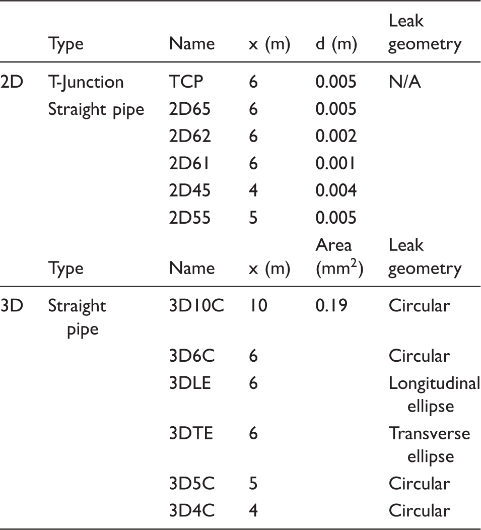
The commercial ANSYS FLUENT (CFD) code was used to simulate different pipeline systems. In this study, two general types of computational domains have been assessed: a T-Junction (Figure 1(a)) and a straight pipe (Figure 1(b)). Several leak properties have been investigated by changing the leak diameter (d) and the distance of the leak from the inlet (x) in a straight pipe. Table 1 summarises the properties of each case and its corresponding computational domain.

Figure 1.

Computational domains descriptions: (a) T-Junction, (b) straight pipe. x: distance of the leak from the inlet, d: leak diameter.

Table 1.

Case studies specifications.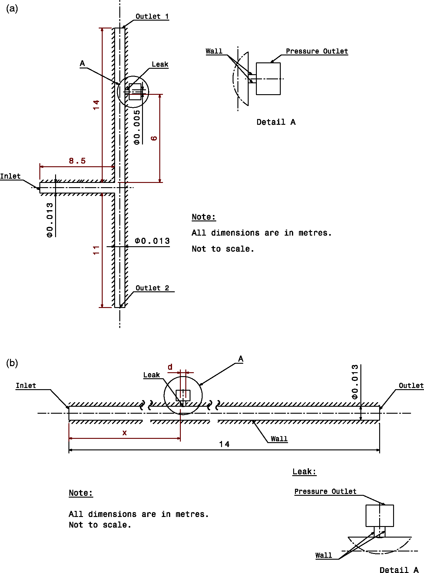

	Type	Name	x (m)	d (m)	Leak geometry
2D	T-Junction	TCP	6	0.005	N/A
	Straight pipe	2D65	6	0.005
		2D62	6	0.002
		2D61	6	0.001
		2D45	4	0.004
		2D55	5	0.005
	Type	Name	x (m)	Area ( $m m^{2}$ )	Leak geometry
3D	Straight pipe	3D10C	10	0.19	Circular
		3D6C	6		Circular
		3DLE	6		Longitudinal ellipse
		3DTE	6		Transverse ellipse
		3D5C	5		Circular
		3D4C	4		Circular

Modelling considerations

In all the simulations, a similar solution method has been applied. Liquid compressible water (using the Tait formulation²⁶) at a temperature of 300 K was used as the working fluid. The density of water, ρ, was set to 998.2 ( $kg / m^{3}$ ), and the water bulk modulus K_W was 2.16 GPa. The theoretical speed of the pressure wave was equal to 1471.7 m/s, using the standard equation, $\sqrt{K_{W} / ρ}$ .

To introduce the transient pressure wave, the inlet pressure from the steady state condition of 15,000 Pa (Re = 83,177) was dropped to 2500 Pa (Re = 33,957) after 22.2 µs.

The boundary condition for the outlets and leaks were set to atmospheric pressure. No-slip boundary conditions were assigned to the walls. It will be noted that both two- and three-dimensional models were conducted. The 2D models were in effect of an infinite flow channel with an slit for the leak. The 3D models were more accurate, with the leak modelled as a hole in the pipe, but these were computationally far more expensive to run.

Solution methods

The standard k-∈ scheme was applied for turbulence modelling.²⁷ The turbulent length scale was set to the internal diameter of the pipe and the turbulent intensity at the inlet was set to 10%. The SIMPLE scheme was used for pressure-velocity coupling. The second-order upwind scheme was used as the discretisation method for the momentum, turbulent kinetic energy and dissipation rates. In the unsteady simulations, the transient formulations (pressure, momentum, turbulent kinetic energy and turbulent dissipation rate) were set to second-order.

After comparing a wide range of structured quadrilateral mesh densities, meshes with 6000 and 180,000 nodes for 2D and 3D straight pipelines, respectively, were selected, whilst the mesh density for the T-Junction case was about 7000 nodes. In these unsteady cases, the time step of $10^{- 5}$ s was deemed to be acceptable to capture the key flow features.

Results and discussion

Figure 2 shows the variation of the introduced transient wave at different positions of the straight pipe computational domain. The original defined inlet pressure profile is shown in Figure 2(a). Figure 2(b) highlights the measured profile at the inlet sensor, whilst, Figure 2(c) shows the captured transient wave just before a leakage. In Figure 2(c), the introduced transient wave is shown as a sudden pressure drop after about 4 ms, and then after a short delay, the pressure can be seen to increase, due to the arrival of the reflected negative pressure wave from the leak. As the introduced transient wave is the same for all the simulations, one would expect the same type of response for all the T-Junction simulations.

Figure 2.

Transient pressure wave profile: (a) Before the inlet, (b) after the inlet and (c) before a leak.

The introduced transient pressure wave and its reflections were measured 0.01 m after the inlet and before the outlet. Consequently, the cepstrum, the cross-correlation and the cepstrum of cross-correlation signal analysis methods were applied to a variety of cases for both straight pipe and T-Junction geometries and hence computational domains. The results are individually discussed and compared later.

Straight pipe

Different leak properties (size, position and geometry) were numerically simulated in a straight pipeline, both 2D and 3D. The pressure signal 0.01 m after inlet and before the pipe outlet was monitored. The speed of sound inside the pipeline was determined by the time that the introduced transient pressure wave requires to reach the outlet; which gave a celerity of 1471.7 m/s (the signal time is converted to distance using this value). The measured celerity is equal to the theoretical value, which is given in the ‘Modelling considerations’ section of the paper.

The cepstrum method

The cepstrum of the inlet pressure signal on its own is used to estimate the leak location in the straight pipeline cases (Figure 3). A very sharp peak can be observed at the distance from each of the leaks to the inlet sensor. Figure 3(a) shows the results for 2D cases with different leak size at 6 m from the inlet, the leak is predicted with a slight variation of 1% in all cases. The cepstrum results for different leak positions in both 2D and 3D simulations are shown in Figure 3(b) to (d), the errors in predicting the leak location was considerably lower for the 3D cases. Furthermore, changing the leak geometry has not affected the results, the longitudinal and transverse ellipse and the circular leaks were detected with exactly the same precision (1%). Comparing the results with Brunone and Ferrante,¹⁸ experimental investigation confirms the dependency of the pressure signal to the leak size. However, changing the leak shape has not affected the results. Overall, the leak at the 3D4C case was detected with the highest accuracy (0.75%), while 2D55 had the worst prediction (2.20%).

Figure 3.

The cepstrum of the inlet pressure signals for different leak geometries: (a) 2D models with different leak sizes, (b) 2D models with leak at different positions in the pipe (4, 5 and 6 m), (c) 3D models with leak at different positions of the pipe (4, 5 and 6 m), (d) 3D models with leak placed at different positions of the pipe (10 m) and (e) 3D leak with various geometries (circular, longitudinal ellipse and transverse ellipse).

The cross-correlation method

The extracted pressure signal from the inlet and outlet sensors were used to calculate the cross-correlation, the results are provided in Figure 4. The time-delay captured within the cross-correlation result has been used to locate the leak position. Changing the leak size has made a minor effect on the signal pattern. As was expected, changing the location of the leak caused a shift in the signal position. In the 3D10C case, the x-axis is given in negative values, since the leak was more closer to the outlet sensor than the inlet. Overall, the positions of the leaks are slightly over-predicted by about 1.5%, except for the 3D10C, 2D61 and 2D62 cases.

Figure 4.

The cross-correlation results for different leak geometries: (a) 2D cases with different leak sizes, (b) 2D cases with a leak placed at different positions in the pipe (4, 5 and 6 m), (c) 3D cases leak placed at different positions of the pipe (4, 5 and 6 m), (d) 3D cases, leak placed at different positions in the pipe (10 m) and (e) 3D leak with various geometries (circular, longitudinal ellipse and transverse ellipse).

The cepstrum of the cross-correlation

Figure 5 is an example (using the 3D4C case) that demonstrates the effectiveness of the cepstrum analysis approach for extracting the periods between the delay peaks of the cross-correlation signal.

Figure 5.

Use of the proposed method for the 3D4C case: (a) Cross-correlation signal and (b) cepstrum of cross-correlation results.

Figure 5(a) shows the cross-correlation signal, and it is possible to observe that the peaks and delay peaks are repeated within certain periods. Considering the periods of 8 m that are highlighted with dashed light grey arrows, the reason for this observation is the transient pressure wave and its reflections are trapped between inlet and leak. This period is clearly identified by the cepstrum of cross-correlation; the largest peak in Figure 5(b). Also, there is a smaller peak around 4 m in the cepstrum figure; this period is shown by the grey arrows in Figure 5(a).

When looking at Figure 3, it can be seen that the most repeated period is roughly equal to the twice distance between the inlet sensor and the leak, so there is going to be a noticeably large peak equal to twice of this distance within the cepstrum results. For a clearer presentation of the results, this periodicity has been removed in all the graphs by dividing the distances by two.

The cepstrum of cross-correlation results for different leak sizes (2D61, 2D62 and 2D65) are shown in Figure 6(a). The signal patterns are almost unaffected; however, the amplitudes varied noticeably. The highest amplitude is observed for the largest leak size (2D65), while the smallest leak (2D61) has generated a larger amplitude signal than the medium one (2D62). It is therefore not yet possible to estimate the leak size based on the amplitude of the output signal. The smaller leak is detected with considerably higher accuracy (less than 0.6% error), while in the 2D62 case, the leak is over-predicted by about 1.8%. Figure 6(b) to (d) shows the results of the cepstrum analyses for a single leak size at different positions in the pipe from both 2D and 3D simulations, respectively. For both 2D and 3D cases, the analysis has shown large peaks at the distance to the leak position from the inlet. For both the 3D4C and 2D45 cases, the largest peak is located around 4 m and the leaks were detected with 0.5% and 0.75%, accuracy, respectively. Interestingly, the peak for 2D55 has captured two reflections (a double peak) at this point; this could be due to the resolution and the sensor positions, such that signal of the leak is spread across two time steps. The errors for identifying the leaks in 2D55 and 3D5C were 1% and 0.4%, respectively.

Figure 6.

The cepstrum results for different leak geometries: (a) 2D models with different leak sizes, (b) 2D models with leak at different positions in the pipe (4, 5 and 6m), (c) 3D models with leak at different positions of the pipe (4, 5 and 6 m), (d) 3D models with leak at different positions of the pipe (10 m) and (e) 3D leak with various geometries (circular, longitudinal ellipse and transverse ellipse).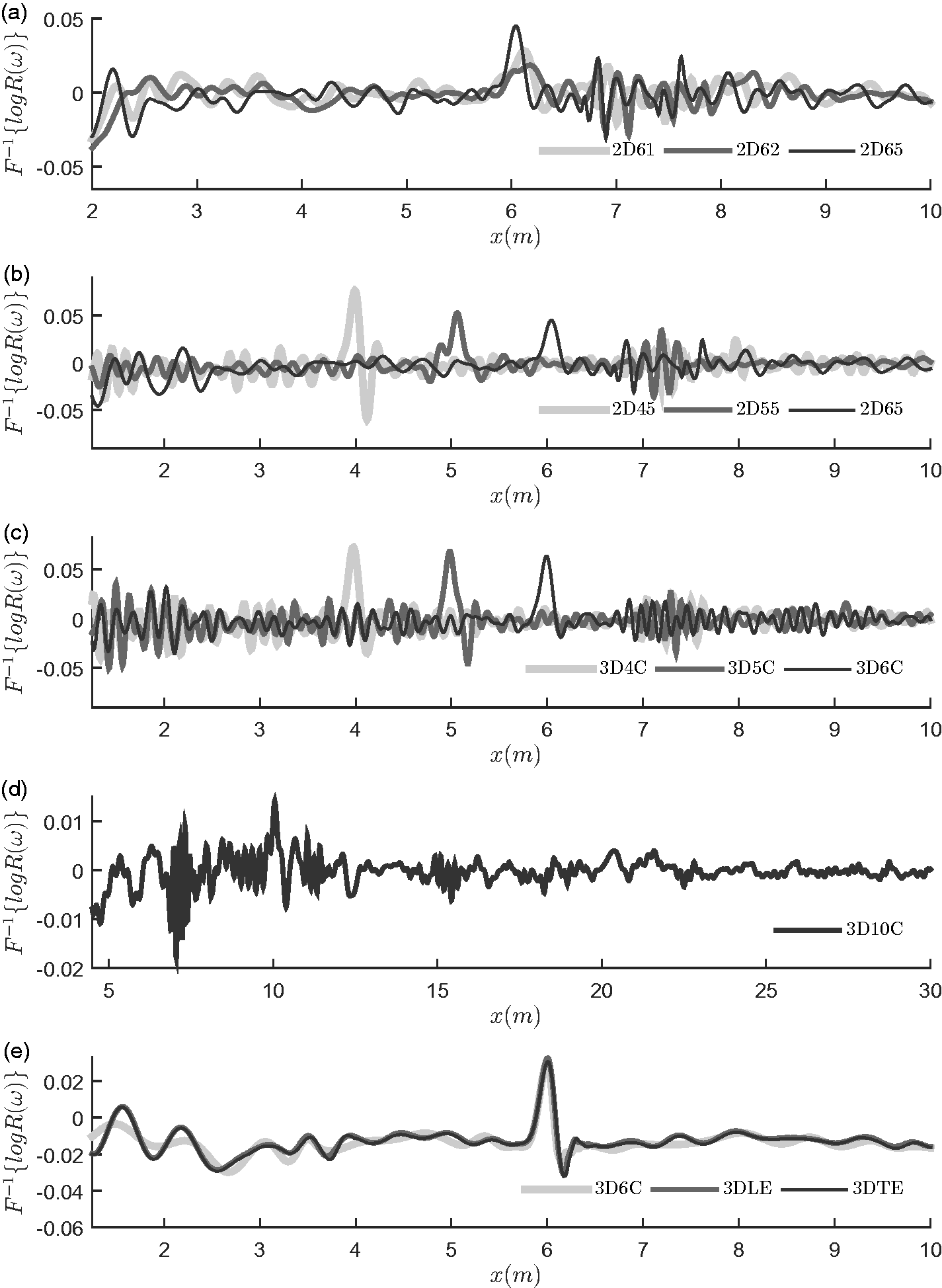

Finally, the peak describing the leak at 6m streamwise is observed around 6m in both 2D65 and 3D6C (0.17%). Considering the case where the leak is located at 10 m (3D10C) in Figure 6(d), the output signal can be seen to fluctuate, which is because the leak position is close to the outlet where reflections will occur. A peak can be identified at around 10 m and this leak is detected with a 1.4% error. Furthermore, the signal attenuation rate was higher in the 2D cases and double peaks were also mainly observed in 2D cases (2D62 and 2D55).

Figure 6(e) shows that the output signal for the leaks with different shapes have a very similar pattern. The output for the circular leak had more fluctuations than the other cases, although the errors for detecting the leak were similar in all cases and equal to 0.17%. The proposed method is not sensitive to leak shape and it is able to identify leaks, regardless of their geometry.

Idealised pressure signals

The signal processing methods are also tested on two idealised pressure signals. It is possible to approximately estimate the time that the pressure waves are going to be sensed near the inlet and outlet of a straight pipe. Therefore, two idealised pressure signals for a straight pipe with a leak placed 4 m downstream of the inlet were created. Figure 7(a) and (b) shows the idealised inlet and outlet pressure waves signals compared to the CFD simulation results, respectively. Note the time is converted to distance by having the speed of the pressure wave.

Figure 7.

Idealised inlet and outlet pressure waves simulated for a straight pipe with a leak placed 4 m upstream from the inlet compared to measured signals in the CFD simulation. CFD: computational fluid dynamics.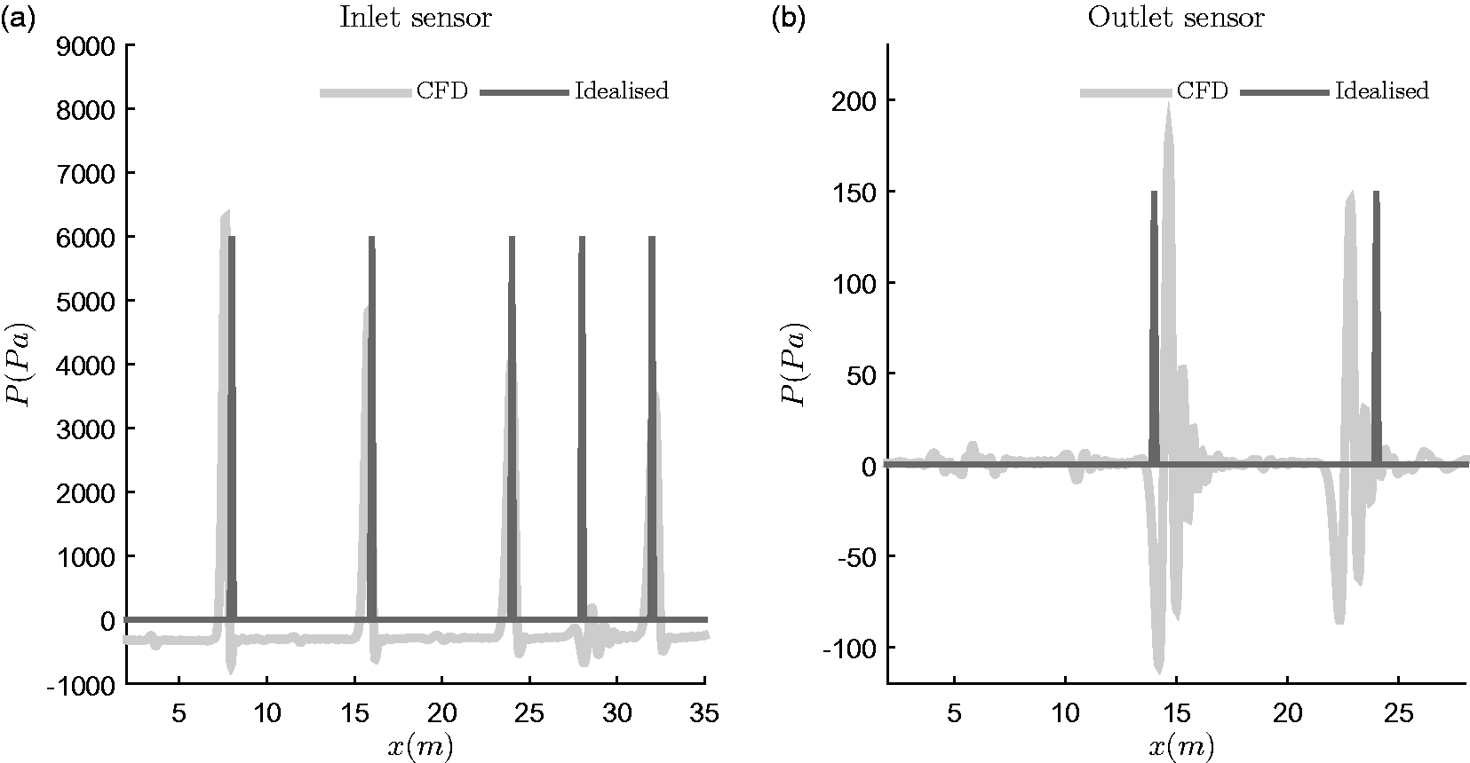

The idealised pressure signals are used to calculate cepstrum, cross-correlation and cepstrum of cross-correlation. The results of the analysis can be found in Figure 8. Comparing the results with the CFD simulation data shows a close estimation of the locations that the peaks were expected.

Figure 8.

Idealised inlet and outlet pressure waves created for a straight pipe with a leak placed 4 m upstream from the inlet compared to measured signals in the CFD simulation. CFD: computational fluid dynamics.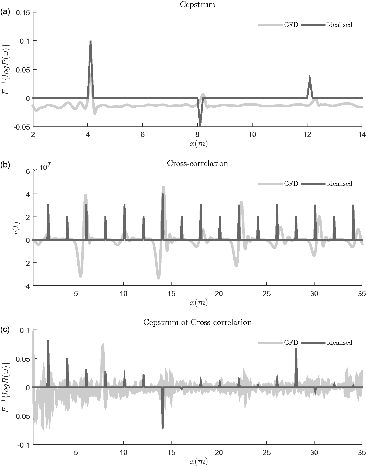

Comparing the methods

Table 2 shows the numerical calculations for each case, using different signal processing methods. The first column introduces case specifications, while the actual and predicted location of the leaks are given in the X_a and X_p column, respectively. Finally, the errors are shown in the last column for each method.

Table 2.

The results of cross-correlation, cepstrum and cepstrum of cross-correlation leak detection methods.

Case Specifications		Cross-correlation		Cepstrum of Pressure		Cepstrum of Cross-correlation
Name	X_a (m)	X_p (m)	Error (%)	X_p (m)	Error (%)	Xp	Error (%)
3D6LH	6	6.09	−1.50	6.06	−1.00	5.99	0.17
3D6TE	6	6.08	−1.33	6.06	−1.00	5.99	0.17
3D6C	6	6.09	−1.50	6.06	−1.00	5.99	0.17
3D4C	4	4.06	−1.50	4.03	−0.75	3.97	0.75
3D5C	5	5.07	−1.40	5.04	−0.80	4.98	0.40
3D10C	10	9.8	2.00	10.03	−0.30	10.14	−1.40
2D61	6	5.95	0.83	6.05	−0.83	6.03	−0.50
2D62	6	5.95	0.83	6.13	−2.17	6.11	−1.83
2D45	4	4.15	−3.75	4.04	−1.00	3.98	0.50
2D55	5	5.07	−1.40	5.11	−2.20	5.05	−1.00
2D65	6	6.29	−4.83	6.08	−1.33	6.01	−0.17

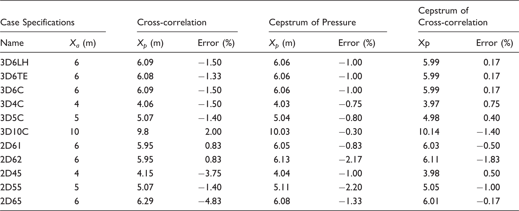
X_a: actual leak location; X_p: predicted leak location.

T-Junction

Two T-Junction cases, with and without a leak were studied. Two “sensors” were used to capture the static pressure signal, 0.01 m after the inlet and 0.01 before the downstream outlet (outlet 2 in Figure 1). The speed of the pressure wave was estimated to be equal to 1471.7 m/s.

Figure 9(a) represents the cross-correlation outputs. The position of the leak and the outlet can clearly be identified around 14 and 19.4 m, whilst the position of the junction is not clearly observed. On examining the cepstrum of the inlet pressure (Figure 9(b)), the position of junction, leak and outlet are all predicted with less than a 0.5% error.

Figure 9.

The results for T-Junction cases: (a) Cross-correlation signal, (b) cepstrum and (c) cepstrum of cross-correlation.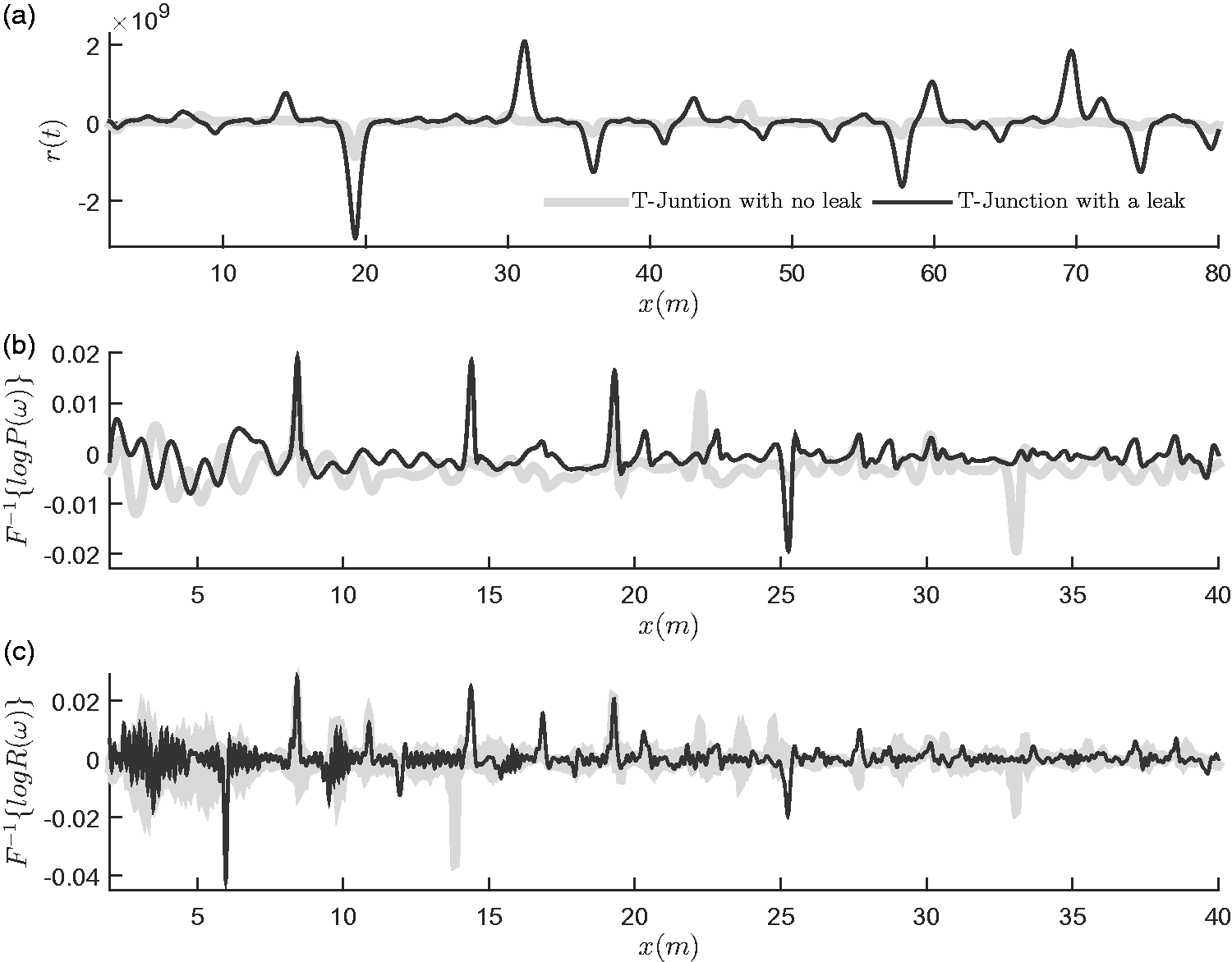

The cepstrum of the cross-correlation is shown in Figure 9(c). Four sharp peaks are noticeable at the beginning of graph; the first peak, about 6 m, is related to the distance between the junction and leakage. This peak is negative as positive reflections from the leak or a junction will give the opposite sign in the cross correlation to an open end. Furthermore, the second peak around 8.5 m identifies the junction with a 0.71% error, the third predicts the leak location (about 14.4 m) with a 0.21% error, and finally, the outlet (near 19.5 m) position is located within 0.5%. (Details of the results can be found in Table 3).

Table 3.

T-Junction results.

Case specification		Cross-Correlation		Cepstrum of Pressure		Cepstrum of Cross-correlation
Name	X_p (m)	X_p (m)	Error (%)	X_p (m)	Error (%)	X_p (m)	Error (%)
Junction	8.4	–	–	8.42	0.24	8.46	0.71
Leak	14.4	14.36	0.28	14.41	0.07	14.37	0.21
Outlet	19.4	19.32	0.41	19.29	0.57	19.3	0.52

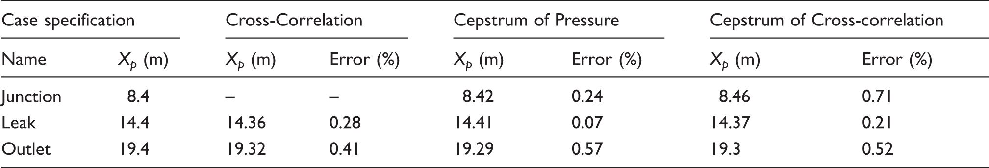
X_a: actual leak location; X_p: predicted leak location.

It can be seen from this that the cepstrum result is clearest for the 3D case. The accuracy of both the cepstrum and the cross correlation of the cepstrum are good with a slightly better location shown by the cepstrum. Not surprisingly, as the cepstrum of the cross-correlation should pick up the resonances within the system, it finds the distance between the leak and the junction as an additional peak. This indicates that there is a lot of information in the signals, which can be extracted using signal analysis techniques.

For these more complicated systems, it may be useful to use a variety of techniques and find the common peaks to identify features with greater surety. In the cases shown above, this would be particularly useful in removing the spurious peaks from the non leak analyses in Figure 9(b) and (c).

Conclusions

An improved transient leak detection method is introduced, which is based on the cepstrum of the cross-correlation of the signals upstream and downstream of the leak. Different leak properties are simulated within a straight pipe and a T-Junction system. This novel technique is more accurate than the cross-correlation and cepstrum results on their own for a straight pipe. However, for more complicated systems, the number of peaks increases and it is harder to discern features for certain. The cepstrum of the cross-correlation method is more accurate than using the cross-correlation alone, since it picks up the periodicity in the cross correlations.

Changing the leak position in both 2D and 3D simulations showed that there was a more accurate prediction resulting from the 3D cases, showing the importance of good data for the signal analysis techniques. A 3D leak gives a sharper (though smaller) reflection. When the location was kept the same and the leak size was altered, the prediction error was fundamentally unchanged. From the work shown here, there does not appear to be a straightforward method to ascertain the leak flow rate based on this method.

The proposed technique is not sensitive to the leak's geometry as it has predicted different leak shapes with roughly the same precision. It is relatively simple to pick up multiple features using this approach. For example, in the case of a T-Junction network with a leak, both features were detected with approximately a 1% error; however, it was not always clear what was a relevant peak in these more complicated systems.

Footnotes

Declaration of Conflicting Interests

The author(s) declared no potential conflicts of interest with respect to the research, authorship, and/or publication of this article.

Funding

The author(s) received no financial support for the research, authorship, and/or publication of this article.

Appendix

References

Colombo

Lee

Karney

. A selective literature review of transient-based leak detection methods. J Hydro-Environ Res 2009; 2: 212–227.

Wylie

Streeter

Suo

. Fluid transients in systems 1993; vol 1, Englewood Cliffs, NJ: Prentice Hall.

Wylie EB and Streeter VL. Fluid transients. New York: McGraw-Hill International Book Co., 1978, p. 401.

Lighthill

. Waves in fluids, Cambridge: Cambridge University Press, 2001. .

Thorley

. Fluid transients in pipeline systems, New York: ASME Press, 2004.

Beck

Williamson

Sims

et al.

Pipeline system identification through cross-correlation analysis. Proc IMechE, Part E: J Process Mechanical Engineering 2002; 216: 133–142.

Beck

Curren

Sims

et al.

Pipeline network features and leak detection by cross-correlation analysis of reflected waves. J Hydraul Eng 2005; 131: 715–723.

Taghvaei

Beck

Staszewski

. Leak detection in pipelines using cepstrum analysis. Measure Sci Technol 2006; 17: 367–372.

Ghazali

Beck

Shucksmith

et al.

Comparative study of instantaneous frequency based methods for leak detection in pipeline networks. Mech Syst Signal Process 2012; 29: 187–200.

10.

Ferrante

Brunone

Meniconi

. Wavelets for the analysis of transient pressure signals for leak detection. J Hydraul Eng 2007; 133: 1274–1282.

11.

Ferrante

Meniconi

. Leak-edge detection Détection des fuites-contours. J Hydraul Eng 2009; 47: 233–241.

12.

Ferrante

Capponi

Collins

et al.

Numerical transient analysis of random leakage in time and frequency domains. Civil Eng Environ Syst 2016; 33: 70–84.

13.

Hanson

Randall

Brown

et al.

Locating leaks in underground water pipes using the complex cepstrum. Austr J Mech Eng 2008; 6: 107–112.

14.

Motazedi N and Beck SBM. The use of the cross-correlation of two signals as a transient leak detection method. In: BHR Group - 12th International conference on pressure surges, Dublin, Ireland, 2016, pp.581–594.

15.

Watton

Pham

. Fault classification of fluid power systems using a dynamics feature extraction technique and neural networks. Proc IMechE, Part I: J Systems and Control Engineering 1998; 212: 87–97.

16.

Wiener

. Extrapolation, interpolation, and smoothing of stationary time series 1966; vol 2, Cambridge, MA: MIT Press.

17.

Taghvaei

Beck

Boxall

. Leak detection in pipes using induced water hammer pulses and cepstrum analysis. Int J COMADEM 2010; 19: 25.

18.

Brunone

Ferrante

. Detecting leaks in pressurised pipes by means of transients. J Hydraul Eng 2001; 39: 539–547.

19.

Lange

Johns

. Correlation techniques, London: Iliffe, 1967.

20.

Oppenheim AV. Superposition in a class of nonlinear systems. Massachusetts: MIT Research Laboratory of Electronics, 1965.

21.

Kemerait

Childers

. Signal detection and extraction by cepstrum techniques. IEEE Trans Inform Theory 1972; 18: 745–759.

22.

Childers

Skinner

Kemerait

. The cepstrum: A guide to processing. Proc IEEE 1977; 65: 1428–1443.

23.

Senmoto

Childers

. Adaptive decomposition of a composite signal of identical unknown wavelets in noise. IEEE Trans Syst Man Cybernet 1972; 1: 59–66.

24.

Bogert BP, Healy MJ and Tukey JW. The quefrency alanysis of time series for echoes: Cepstrum, pseudo-autocovariance, cross-cepstrum and saphe cracking. In: Proceedings of the symposium on time series analysis, New York, Vol. 15, 1963, pp.209–243.

25.

Randall RB. A history of cepstrum analysis and its application to mechanical problems. In: International conference at Institute of Technology of Chartres, France, 2013, pp.11–16.

26.

Hayward

ATJ

. Compressibility equations for liquids: a comparative study. Br J Appl Phys 1967; 18: 965–977.

27.

Jones WP and Launder BEi. The prediction of laminarization with a two-equation model of turbulence. Int J Heat Mass Transf 1972; 15: 301–314.

Leak detection using cepstrum of cross-correlation of transient pressure wave signals

Abstract

Keywords

Introduction

Methodology

Cross-correlation

Complex cepstrum

Numerical simulations

Modelling considerations

Solution methods

Results and discussion

Straight pipe

The cepstrum method

The cross-correlation method

The cepstrum of the cross-correlation

Idealised pressure signals

Comparing the methods

T-Junction

Conclusions

Footnotes

Declaration of Conflicting Interests

Funding

Appendix

References