
Abstract
The most common simulation approach in rotor dynamics is based on beam models. Usually, these models are very compact and come at low computational costs. However, they are afflicted with a number of limitations, making them insufficient for the analysis of more complex rotor systems, which require 3D solid modeling. General purpose FEM codes offer full 3D solid modeling capabilities, but the question still remains, whether they are capable of correctly taking into account all the effects that arise from rotation. This paper provides an example of a complex, highly nonlinear rotor system, which cannot be simulated or even modeled accurately by using beam elements, but rather requires 3D solid modeling. ABAQUS is used-as a representative example for a general purpose FEM code-to build up an appropriate model. By doing so, the paper addresses the question, whether a general purpose FEM code is able to cover the necessary rotor dynamic effects. The model which is derived here takes into account nonlinear stiffness behavior, and includes contact between different components of a rotor assembly. The objective is to simulate a run-up through a bending resonance, using direct time integration. The simulation results are compared with experiments, showing good consistency. During the crossing of the critical speed due to the bending resonance, mode-locking can be observed in the experiment and is well represented by the simulation model.
Introduction
The finite element method (FEM) has become a powerful tool for researchers and engineers to perform rotor dynamic analysis. Although general purpose FE codes offer full 3D solid modeling capabilities to analyze structural dynamic problems, the most common approach in rotor dynamics consists of using beam-element models,1,2 by some authors referred to as shaft-line models. 3 The name arises from the process of creating the mesh by simply placing nodes along the shaft line. These models are very compact, consisting mainly of beam elements and concentrated masses equipped with moments of inertia to account for the gyroscopic effects. Timoshenko beams should be used, since shear deformation can have a strong influence on critical speeds, 4 which is neglected in Euler beams. Spring elements and joints can be added to account for elastic bearing behavior.
For many applications, such models may be sufficient since they are providing the advantages of an intuitive geometric interpretation and low computational costs. However, the simplifications that are necessary to apply a beam model lead to a number of limitations. From a mathematical point of view, there are three major limitations to classical, axisymmetric beam models. At first, they assume the rotor-bearing-foundation system to be linear. At second, they assume that the rotor’s cross-section remains fixed, and that plain cross-sections remain plane in deformed configuration. This is an assumption which is violated at sections with sudden changes in diameter. 5 The third assumption is that there is no coupling between the lateral, axial, and torsional movement of the rotor. As will be shown in the further course of this paper, the outlined example does not fulfill any of these requirements, and therefore requires a more complex approach.
From a more industrial engineering point of view, the most important drawback of beam models is that they cannot be built up automatically from a CAD model, but rather need to be derived manually. This can be a very tedious and time-consuming task. For more complex rotor systems, it is a common practice to set up a detailed 3D solid FE model in order to validate the beam model (in standstill condition).6–9 The simpler beam model is then used, to examine the critical speeds and the loads on the system during rotation. These load cases are afterward returned to the detailed 3D model for a stress and lifetime analysis. If the results require a design change, the beam model needs to be updated and the procedure starts over again. This stepping back and forth between two different simulation approaches can be very time-consuming, and since the two simulations usually require different software programs, the procedure is prone to errors. The interaction between the two models in the approach mentioned previously is indicated in Figure 1.
Flow chart of the role of structural dynamics in the design process of rotating machinery.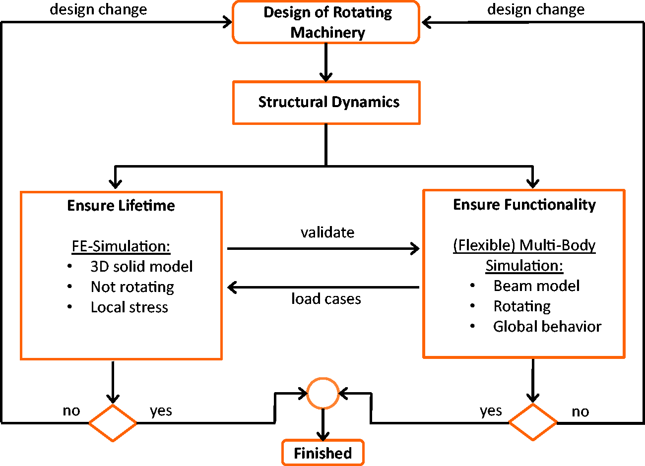
As a consequence and alternative, a detailed 3D solid model could be chosen for the rotor dynamic analysis. One problem might be that solid modeling of a geometrically complex structure requires the use of a commercial program. In the past, a number of known rotor dynamic specialists had their doubts, whether these general purpose FE codes were able to produce correct results when dealing with rotor dynamics. They raised the objections—being right at that time—that these programs lack gyroscopic element formulations and the capability of distinguishing between rotating and nonrotating damping.2,10 Within the last few years, these limitations are claimed to be resolved for some of the most commonly used programs such as ANSYS, 11 ABAQUS, 12 and NASTRAN, 13 which are providing extended rotor dynamic capabilities now. Since in some cases these improvements have been added only in the last couple of years, the number of applications is still limited.
This paper deals with a complex and highly nonlinear rotor system which is shown in Figure 2 and will be described in detail in the next chapter. The nonlinearity arises mainly from the contact situation in the force-locked coupling. Other sources of nonlinearity are the load-displacement curves of the roller bearings and the large displacements of the rotor support foundation (housing). In addition to the nonlinearities, part of the rotor system is asymmetric. The complexity of the system and the number of nonlinearities require the use of solid 3D modeling. ABAQUS is used to develop a 3D solid model, and the simulation results are compared with experimental data. Focus of the research is a bending resonance that occurs during run-up. If the clamping force of the force-locked coupling is exceeded during run-up, mode-locking can be observed in the experiment and is well represented in the simulation model.
Schematic diagram of the outlined rotor system.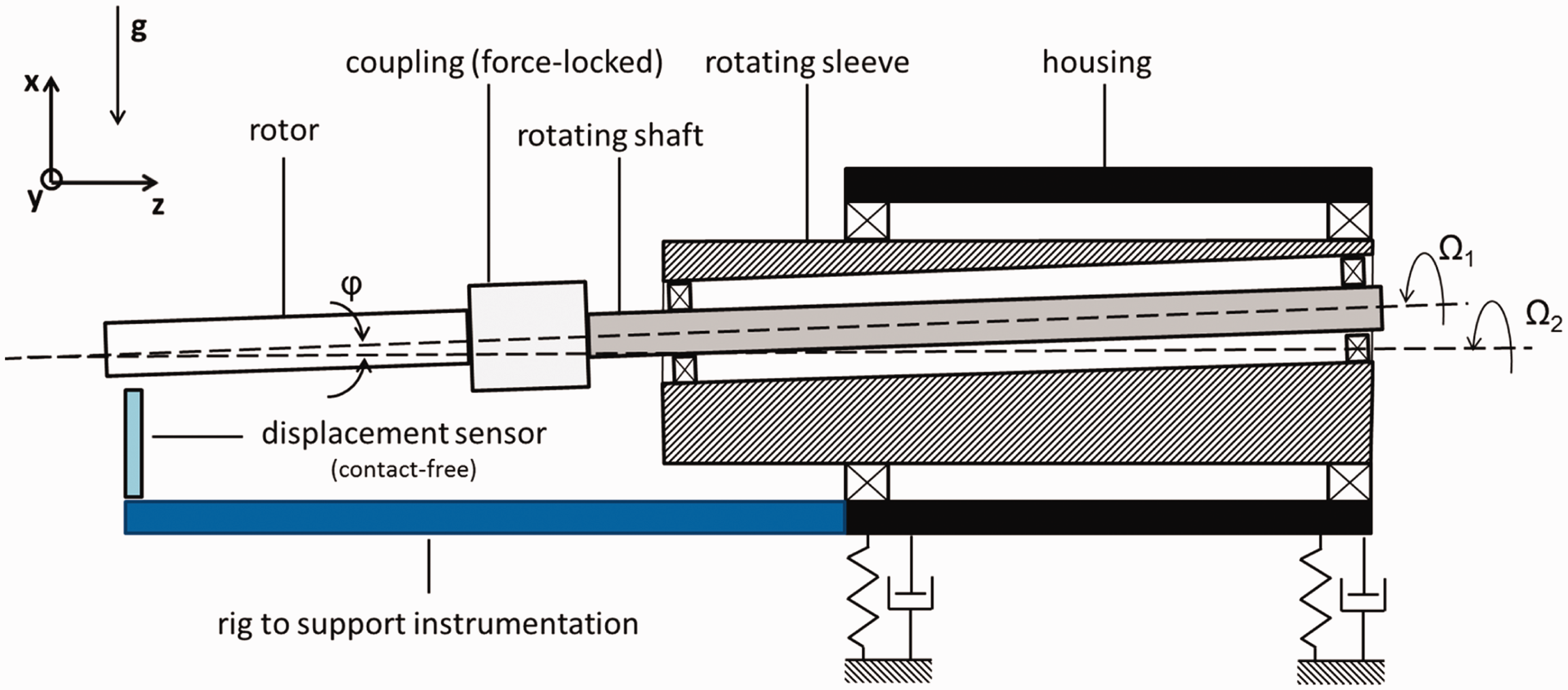
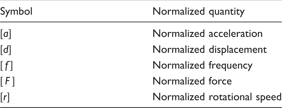
Symbols of normalized quantities.
The outlined rotor system
A schematic diagram of the considered rotor system is shown in Figure 2. At first, the rotor system will be described in general by going from the inside to the outside of the system. After that, some components are described in more detail; especially the force locked coupling needs to be further explained.
The heart of the system consists of a rotor, which is connected to a rotating shaft by a coupling. The three components rotor, coupling, and shaft form a subsystem, which will be referred to as drive shaft, and can be considered as an overhung rotor. The shaft is supported by roller bearings in a sleeve, which is also rotating, but at a lower speed. The bore of the sleeve, in which the shaft is rotating, is not coaxial to the sleeve’s axis of rotation, but has an offset and is twisted by an angle ϕ. This causes the drive shaft to rotate around its own spinning axis, and in addition to perform a tumbling movement around the sleeve’s axis of rotation. The sleeve is supported by roller bearings in a housing, which is in turn elastically supported. Both, the shaft and the sleeve, are driven by an electric motor. The ratio between the turning speed of the shaft (
The coupling, which connects the rotor to the shaft, has a strong influence on the dynamic system behavior and needs further explanation. For reasons of confidentiality, no pictures of the real machine can be shown at the current date. Instead, sketches and sectional views of the FE model are used. Figure 3 shows the rotating parts of the machine and a close-up of the coupling. Figure 4 holds a sectional view of the coupling. The coupling consists of an inner and an outer part, which are pressed axially together by a preloaded disk spring, thereby clamping the connecting end of the rotor in between. The contact between the rotor and the coupling is based mainly on three pins that are evenly spaced in circumferential direction. The part of the rotor, which extends into the inner part of the coupling, is a little smaller in diameter than its counterpart, by this creating a radial clearance. Although the clearance is small, it can lead to a radial misalignment between the rotor and the coupling or the shaft, respectively, depending on how the rotor is mounted.
Sketches of the rotor system with focus on the coupling. Sectional view of the coupling.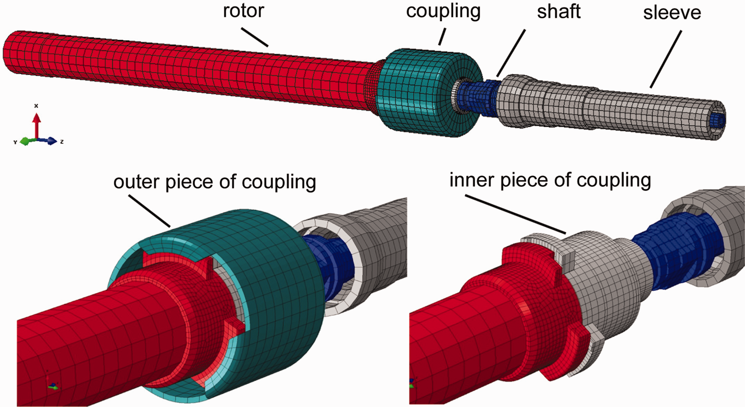
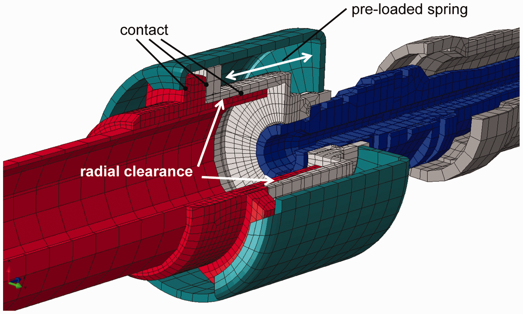
As described, the rotor is held by pressing together the two-piece coupling using a preloaded spring. The three pins of the connecting end of the rotor are clamped axially. The inner part of the coupling is forming sockets around each clip of the rotor. During normal operation, they do not have contact with the coupling in the tangential direction; the torque transfer is ensured purely by friction. It is important to notice that in this design, a lateral force to the rotor will result in axial forces on the pins, and therefore on the coupling. This means that the lateral stiffness of the rotor is strongly linked to the axial stiffness of the coupling. Furthermore, since the clamping spring is highly prestressed, the axial stiffness of the coupling will decrease significantly if the preload of the spring is exceeded, thus leading to a decrease in the rotor’s lateral stiffness as well. This regressing stiffness characteristic causes a strong nonlinear system behavior, leading to interesting rotor dynamic effects, as will be shown in the further course of this paper. It should be mentioned, though, that in normal operation, the pre-load of the clamping spring is sufficient to safely hold the rotor and cannot be exceeded. In the context of the underlying research, the preload was reduced significantly for the sake of provoking the above mentioned rotor dynamic effects.
Figure 2 shows schematically the instrumentation used to measure the displacement of the rotor tip relative to the housing. The rig which supports the displacement sensor(s) is assumed to be rigid. It is designed such that the frequency of its first structural resonance is located far above the first bending resonance of the system, which is the focus of this study. The first resonance frequency of the rig is also located well above the main excitation mechanisms that occur during operation, namely the rotational frequency of the rotor and the sleeve.
Modeling of the system
The model is derived using ABAQUS as a commercial FEM program. ABAQUS is not a special rotor dynamic program, but rather a general purpose finite element code. However, its capabilities seem to be sufficient to even deal with the rotor dynamics of a complex rotor system, such as the one presented here.
The single components are modeled using three dimensional solid finite elements, as already shown in Figures 3 and 4. A rather coarse mesh is used to save computation time. Still, the total number of unknowns is approximately 250,000. The primary objective is to accurately describe the global system behavior during run-up and run-down of the rotor system. Once this is achieved, a finer mesh can be used to correctly compute the local stress distribution, for example, for lifetime analysis. Implicit time integration is used to solve the underlying equations. Although the model size seems quite manageable, the computational effort is very high. Simulating a 5 s run-up takes 12–15 days in real time on a high-performance workstation. The simulation time strongly depends on whether the clamping force in force-locked coupling is exceeded during run-up or not, as will be explained later.
The model is developed bottom-up, meaning that each component and some assembly groups are validated by using test data from experimental modal analysis (EMA) or by using forced response function (FRF) measurements. This approach leaves the compliant connections between different components, for example, the force-locked coupling and the roller bearings, as the parameters with the highest uncertainty.
The roller bearings are considered as a spring damper system, and are modeled using the surface, coupling, and connector functionality, as shown in Figure 5.
Schematic diagram of modeling the roller bearings.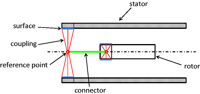
First, a surface is defined for every bearing seat on the shafts or in the housing. The degrees of freedom (DOFs) of the nodes forming a surface are then linked to a single master or reference node, using the coupling function which formulates the necessary kinematic constraints. In turn, the two reference nodes that belong to a corresponding couple of an inner and outer bearing ring (or rather bearing ring seat) are linked by a connector element. The two reference points are positioned at exactly the same geometric position (in undeformed configuration); it is just for better visualization that they have been separated. Going back once more to the coupling function, which creates kinematic constraints between nodes: Different ways of enforcing the corresponding constraints can be chosen. In ABAQUS, the terminus “kinematic coupling” refers to rigid constraints between the master and the coupling nodes, which would turn parts of the shaft and the stator into rigid bodies, therefore increasing the stiffness significantly, depending on the axial length of the defined surface or bearing seat, respectively. As an alternative, ABAQUS offers “distributed couplings” in which the constraints are enforced in an average sense, and in which weighting factors provide control of the load transmission. In the underlying paper, distributed couplings are chosen to model the bearings. This still creates a stiffening effect, which in the end is well appreciated, since it allows to take into account the added stiffness resulting from the press fit of the bearing rings.
The connector element offers manifold possibilities to define the bearing’s stiffness and damping behavior. These dynamic bearing parameters can either be identified by experiments or by using theoretical or numerical models. In the underlying paper, the latter was done. A vast quantity of research has been conducted on how to calculate the dynamic parameters of roller bearings. Literature by Harris and Kotzalas, 14 Jones, 15 Palmgren, 16 and Eschemann et al. 17 on theoretical models is considered to be well accepted by a number of authors. However, while these early models are able to calculate the translational stiffnesses, they lack the capability to accurately estimate the tilting stiffness and the cross-coupling between the different DOFs of a bearing. This insufficiency was overcome, when Lim and Singh18–21 published their model, which was later improved by Liew and Lim. 22 The approach is not only capable of estimating the tilting stiffness of a roller bearing, but can also estimate the cross-coupling between the different DOFs of a bearing. The model provides a fully populated (6 × 6) linearized stiffness matrix (while the line and the column of the DOF of the spinning axis are zero). Successful application of the modeling approach can be found among others in ref. 23 However, the approach by Liew, Lim, and Singh has a major disadvantage: It cannot take into account some geometric data of the bearing rings, which are known to significantly influence the bearing stiffness. 24 Experiments showed that the rotor system regarded here reacts very sensitive to the bearing geometry: Using the same bearing type but from different manufactures results in significant differences with regard to rotor tip displacement during run-up and run-down, indicating that the exact bearing geometry needs to be taken into account. To be able to do so, none of the above-described theoretical models is used. Instead, the load-displacement curves are derived by using 3D solid models of the bearings and performing static load simulations. To determine the exact geometry, the bearings are dissembled and the single parts are measured on a highly precise tactile 3D coordinate measurement machine.
Compared to identifying the stiffness characteristics of a roller element bearing, estimation of damping is more challenging. Most of the available research focuses on experimentally identifying the damping values. A summary and review of relevant articles is presented by Tiwari et al. 25 In this paper, viscous damping is assumed and the damping coefficients of the bearings are determined experimentally by performing a modal analysis when the system is at rest. The in situ approach offers the advantage of taking into account the damping that occurs due to interaction of the bearing races with the housing and the shaft, which is supposed to be significantly larger than the damping that occurs in the bearing itself. 26 According to Kraus et al. 27 the damping of roller element bearings depends strongly on the rotational speed and is decreasing with higher speed. Therefore, the damping in the current paper is probably overestimated, since it is evaluated at standstill condition.
The force-locked connection between the rotor and the coupling is modeled by using one connector element to represent the clamping spring between inner and outer piece of the coupling. The connector is equipped with a load-displacement curve of a preloaded linear spring. The spring parameters have been identified in static measurements. For the interaction between the rotor and the two-piece coupling, contacts are defined at the relevant areas of the different components, as shown in Figure 4. Contacts are defined
between the outer piece of the coupling and the connecting pins of the rotor, between the connecting pins of the rotor and the sockets of the inner piece of the coupling, and between the outer diameter of the connecting end of the rotor and the bore of the inner piece of the coupling. (In undeformed configuration, there is radial clearance between these two contact partners.)
The contact formulations contain friction in which the friction coefficients are taken from the literature 28 according to the combination of materials. In addition to the friction, a small amount of damping is added to the contact behavior. It is only a small value to represent a physical damping effect. The presence of damping significantly increases the convergence.
In nonstationary rotor dynamics, it is important whether the system is controlled through a moment or through displacement or velocity boundary conditions. Here, the electric drive is velocity controlled, but the boundary condition is not applied directly to the engine but through interconnected springs and a dummy mass to allow for elasticity of the drive train.
General dynamic system behavior
Before discussing selected measurements and simulation results in detail, the general dynamic system behavior is described using experimental data.
The system has a bending mode with a frequency located well within the range of rotational speed of the two spinning subsystems, the drive shaft and the sleeve. The mode shape of the vertical bending mode is shown in Figure 6.
Mode shape of the first vertical bending mode.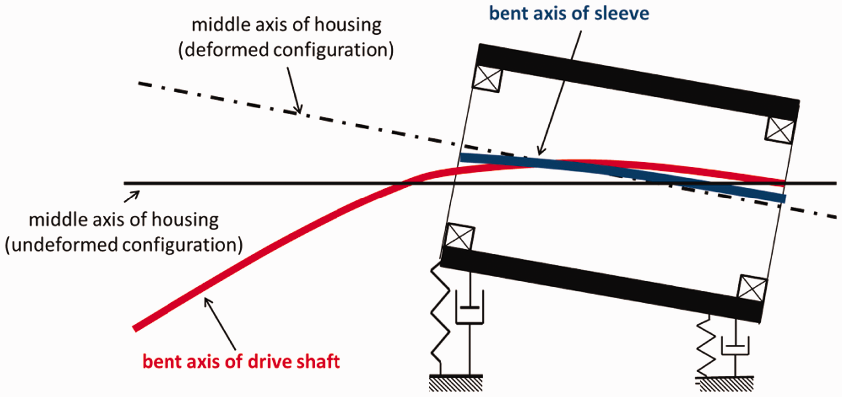
The housing is comparatively stiff with respect to the bending stiffness of the rotating parts and is performing mainly a rigid body motion. However, it is remarkable how much the housing is participating in the mode shape. This is due to the fact that the mass of the rotating parts is large, compared with the mass of the housing. Furthermore, the flexible support of the housing is relatively soft, when compared with the bending stiffness of the drive shaft and the sleeve. The largest deformation comes from the shaft, since it is rather soft with regard to the bending stiffness of the sleeve and the rotor. The housing’s moment of inertia around the y-axis is slightly larger than around the x-axis, causing small anisotropic system behavior. The mode shapes are in principal the same in both vertical (XZ plane) and horizontal (YZ plane) directions, while the latter is appearing at a slightly higher frequency.
The main excitation mechanisms arise from the natural unbalance of the drive shaft and from the tumbling movement, forced by the sleeve. When running up the system, two resonances occur when the rotating frequency of one of the rotors (drive shaft or sleeve) matches the bending frequency of the system. More precisely, it is a matter of four resonances due to the small anisotropic behavior.
The system is equipped with several displacement sensors to measure the relative movement of the rotating parts. In addition, several accelerometers catch the movement of the housing. Figure 7 shows the time signal of the rotor tip displacement in vertical direction relative to the housing during a slow run-up and run-down of the system.
Measurement data—vertical displacement of rotor tip relative to housing during slow run-up and run-down.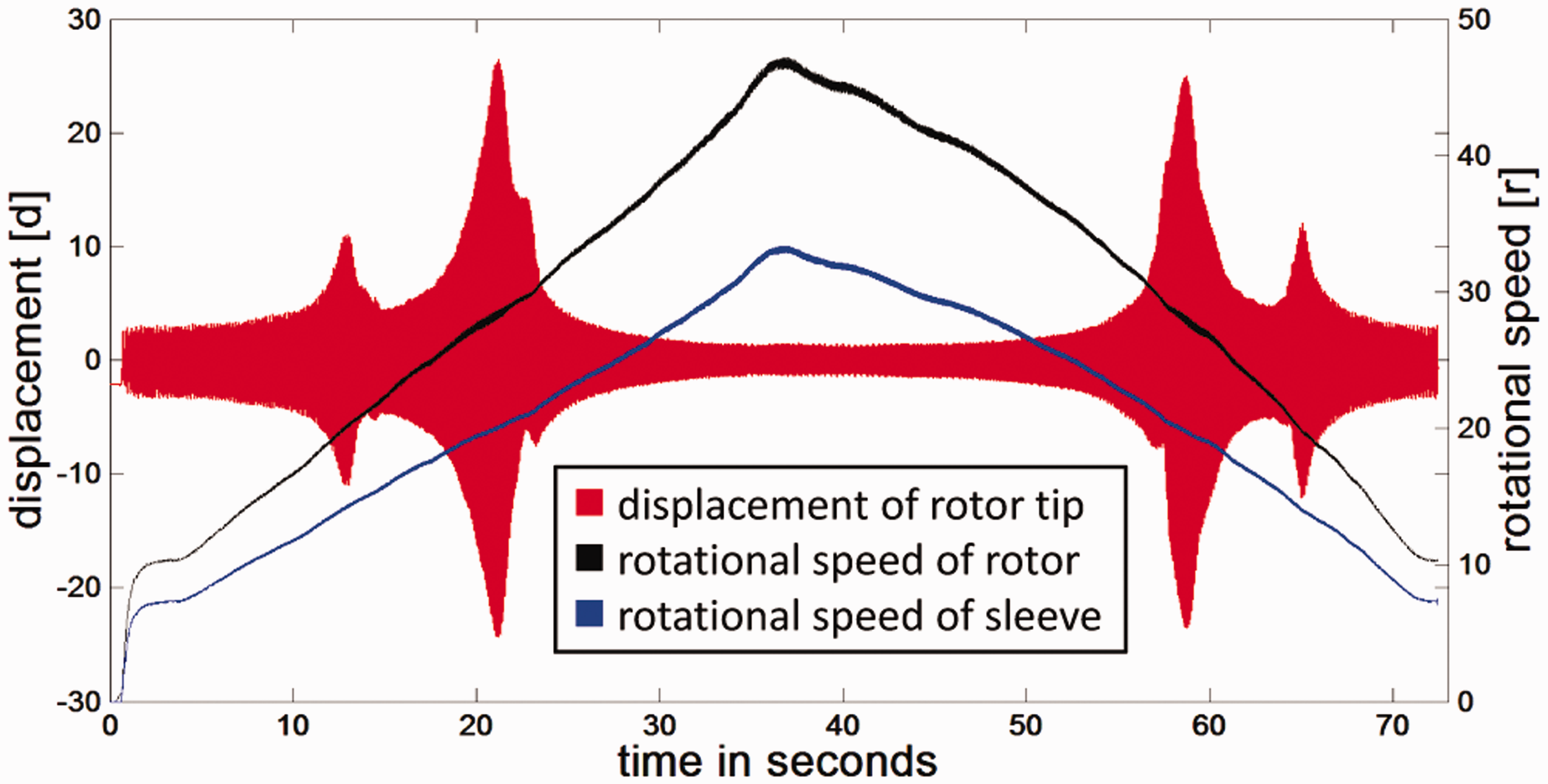
Since the drive shaft is rotating faster than the sleeve, the first resonance peak during run-up can be assigned to the system’s response to the unbalance of the drive shaft. The second peak is caused by the tumbling movement due to the sleeve. In this case, the drive shaft’s unbalance excitation is rather small, compared with the excitation caused by the tumbling.
A maybe more convenient way of presenting the data is to plot the displacement over the rotational speed instead of time. In Figure 8, a vibration order analysis has been performed to calculate the overall displacement level, as well as the share that can be assigned to the first order of the drive shaft and the sleeve. In rotor dynamics, orders are harmonics of the rotational speed, so the terminus “first order” refers to a sinusoidal vibration with the same frequency as the rotational frequency. The order analysis is done by calculating the frequency spectrum at different rotational speeds and cutting out the frequency line that represents the rotational speed of the shaft and that of the tumble sleeve. Since the ratio between the rotational speed of the sleeve and that of the shaft is fixed, according to Equation 1 the first order of the shaft can be considered as the nth order of the sleeve, which allows plotting both orders on the same scaling of the x-axis.
Measurement data—overall level and order plot of vertical displacement of rotor tip relative to housing during slow run-up.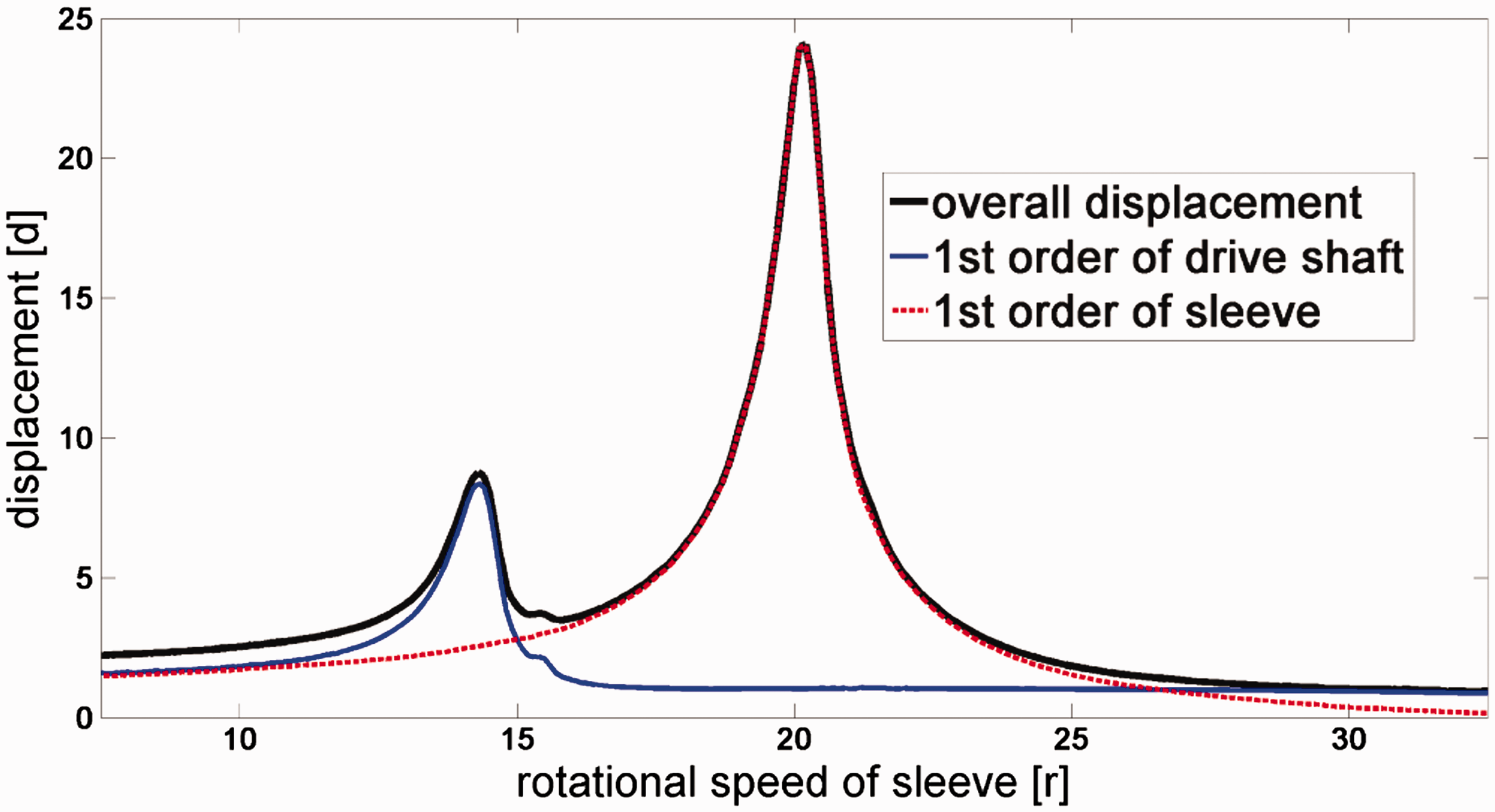
The results in Figure 8 are indicating that the two resonances are well separated, meaning that each resonance is dominated by only one of the two excitation mechanisms.
Figure 9 shows the corresponding Campbell diagram, confirming that the frequency range, relevant for the first bending mode, is clearly dominated by the two excitation mechanisms described above. The two vertical resonances appear at the same frequency.
Measurement data—Campbell diagram of vertical displacement of rotor tip relative to housing during slow run-up.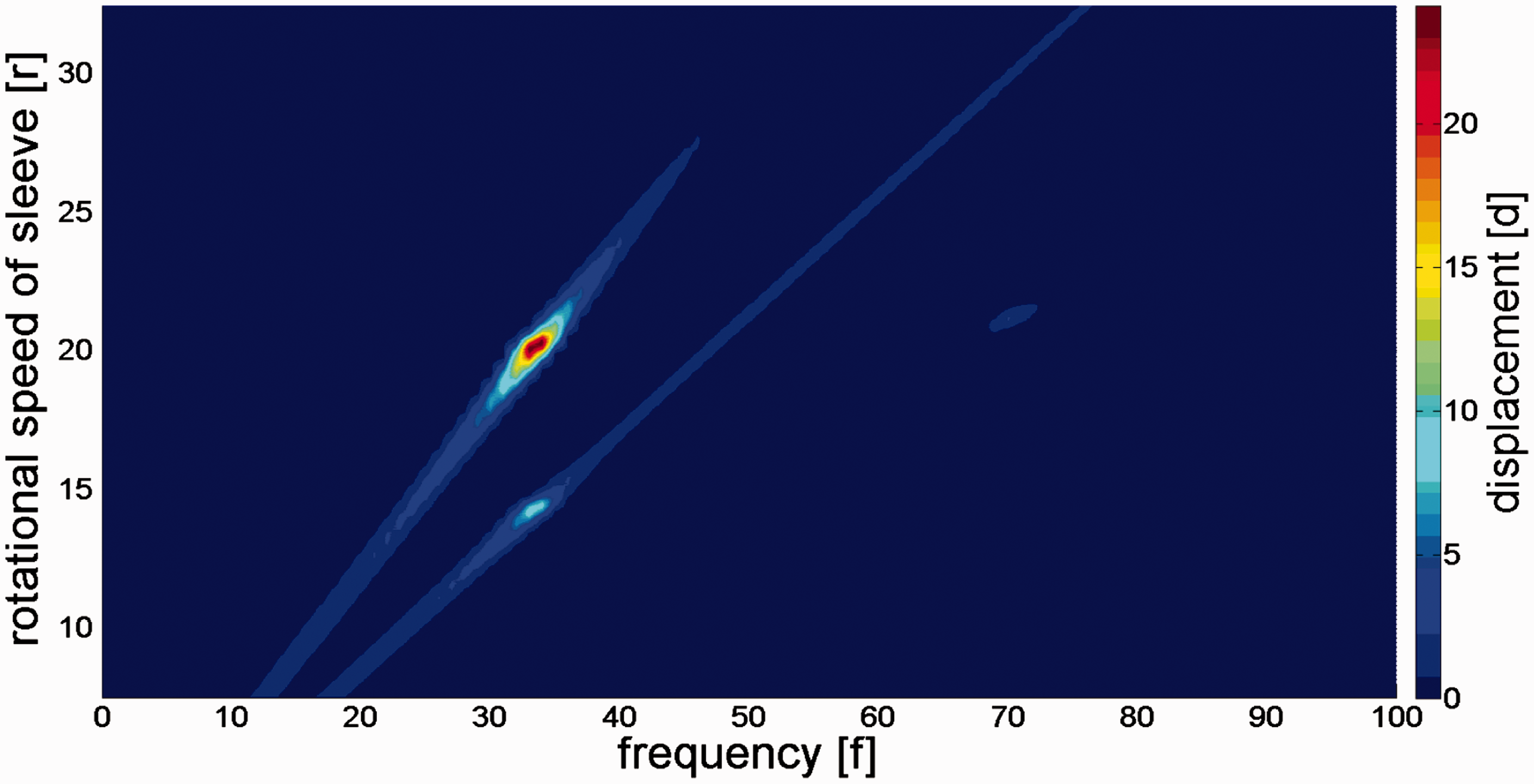
Comparing simulation results to experimental data
In Figure 7, the system was run up and down slowly in order to make the main effects directly visible in the time signal without any further postprocessing. In normal operation, the run-up of the machine is faster. Accordingly, the comparison between experimental data and simulation results in Figure 10 is done, using a shorter run-up time. The experiments are performed with a different rotor, which by chance has a larger natural unbalance than the rotor in Figure 7, therefore leading to a larger amplitude in the first resonance peak. However, it is a coincidence that in the experiment of Figure 10, the first resonance peak, which is caused by the natural unbalance of the rotor, has almost the same amplitude as the second resonance peak, which is caused by the forced tumbling movement of the sleeve.
Comparing simulation results to experimental data during run-up.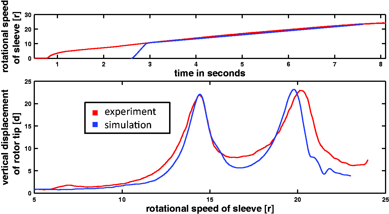
In the simulation, the system is run-up a little faster at the beginning to save simulation time. The comparison between simulation and experiment shows a good consistency. The difference is most likely due to shortcomings in modeling the bearings: To derive the exact geometry of the bearings as described in the modeling part, new bearings were used. In contrast, the experiments were done on a machine, whose bearings had already experienced some operational hours.
Mode-locking due to nonlinear stiffness characteristic
As described in the previous section, the coupling has the potential to create nonlinear system behavior. If the preload of the clamping spring is exceeded, the axial and torsional stiffness will decrease significantly. The effect on the dynamic behavior is at first examined by performing a linearity test, using hammer excitation while the system is not rotating. Figure 11 shows the accelerance FRFs taken at the rotor tip using different levels of excitation force.
Measurement data—accelerance forced response functions taken at the rotor tip with varying excitation force levels [F].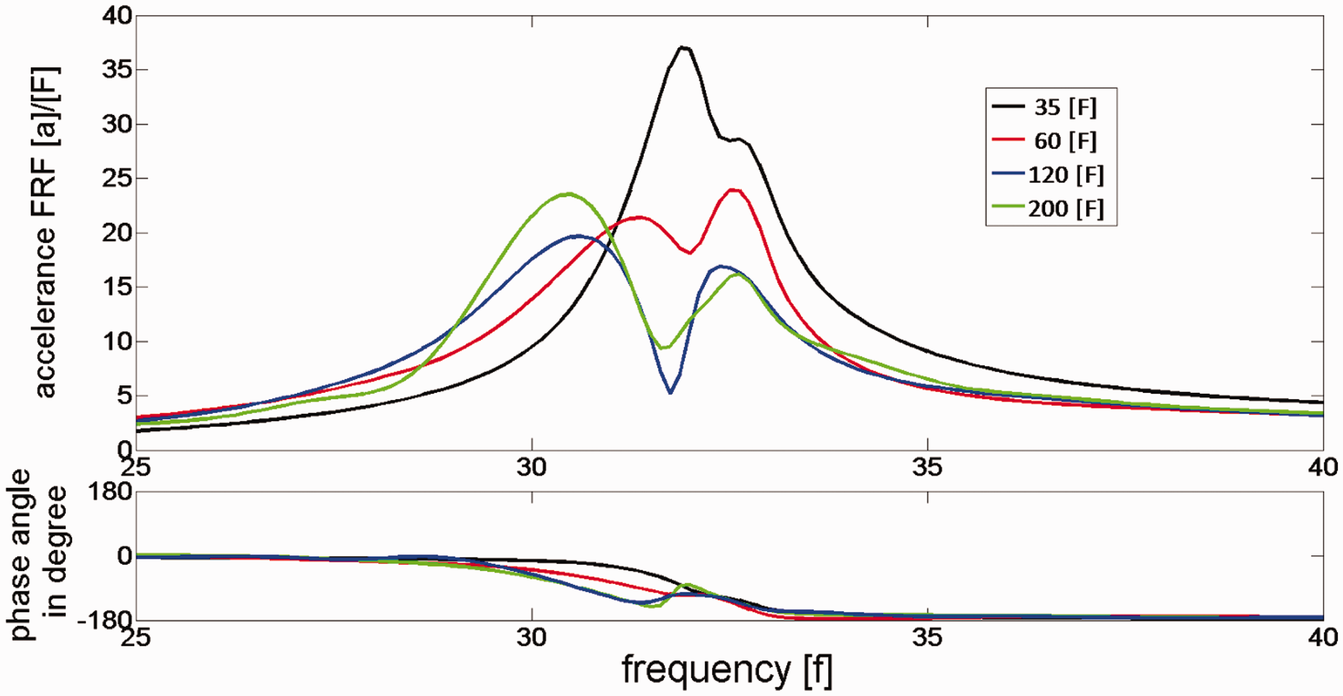
Applying increasing force levels to the rotor tip results in splitting up a former single resonance peak into two peaks, one at a higher and one at a lower frequency than the original peak. The corresponding mode shapes of the two peaks are identical and do not differ from the shape at a very small force. This dynamic behavior is matching well the nonlinear lateral stiffness characteristic of the rotor-coupling subsystem, which is reported in Figure 12 and will be explained in what follows.
Simulation results—lateral stiffness of the rotor in the coupling (load-displacement curve).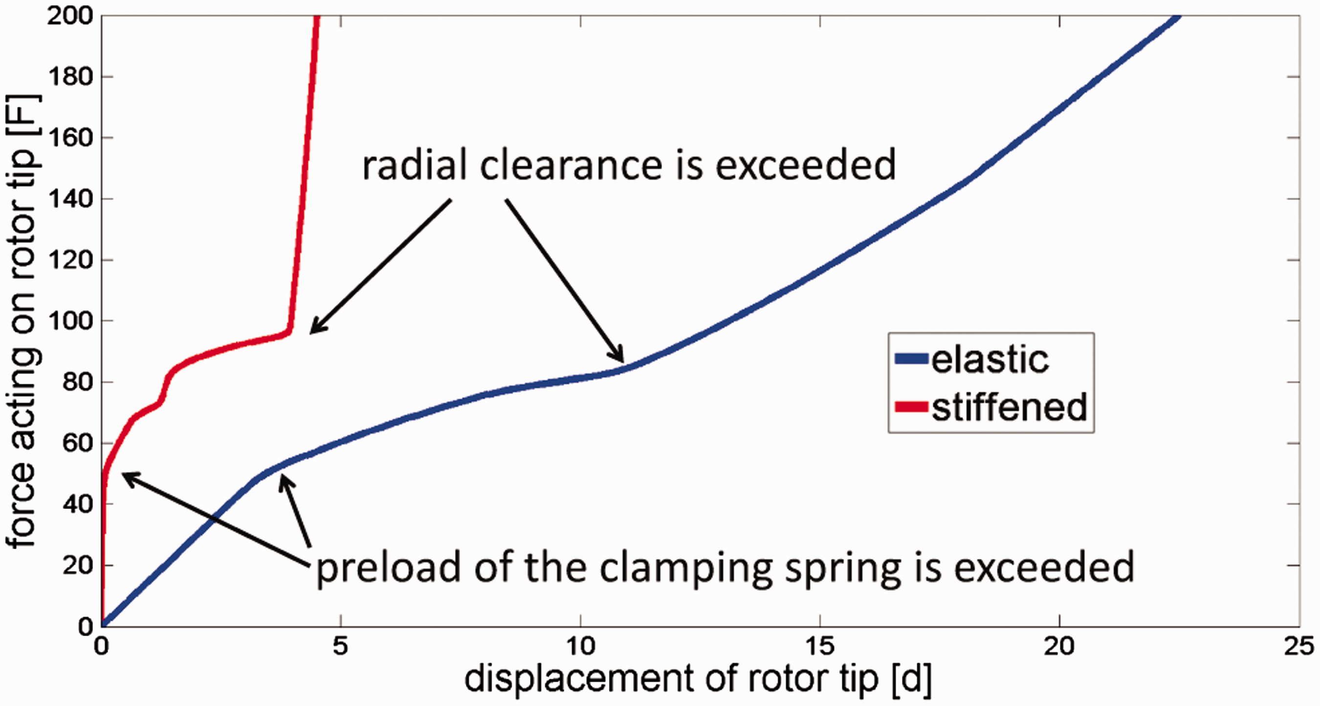
The data for the plot in Figure 12 have been created by applying a linearly increasing, static force to the tip of the rotor, while providing fixed boundary conditions to the inner coupling piece in the connecting area to the shaft. The simulation was carried out twice: first by using realistic, elastic material properties and second by providing an unrealistically high Young’s modulus to simulate stiffened component behavior in order to get the kinematic influence. Figure 13 shows the stress distribution and the contact situation in the elastic simulation.
Contact situation when the rotor is tilted inside of the coupling.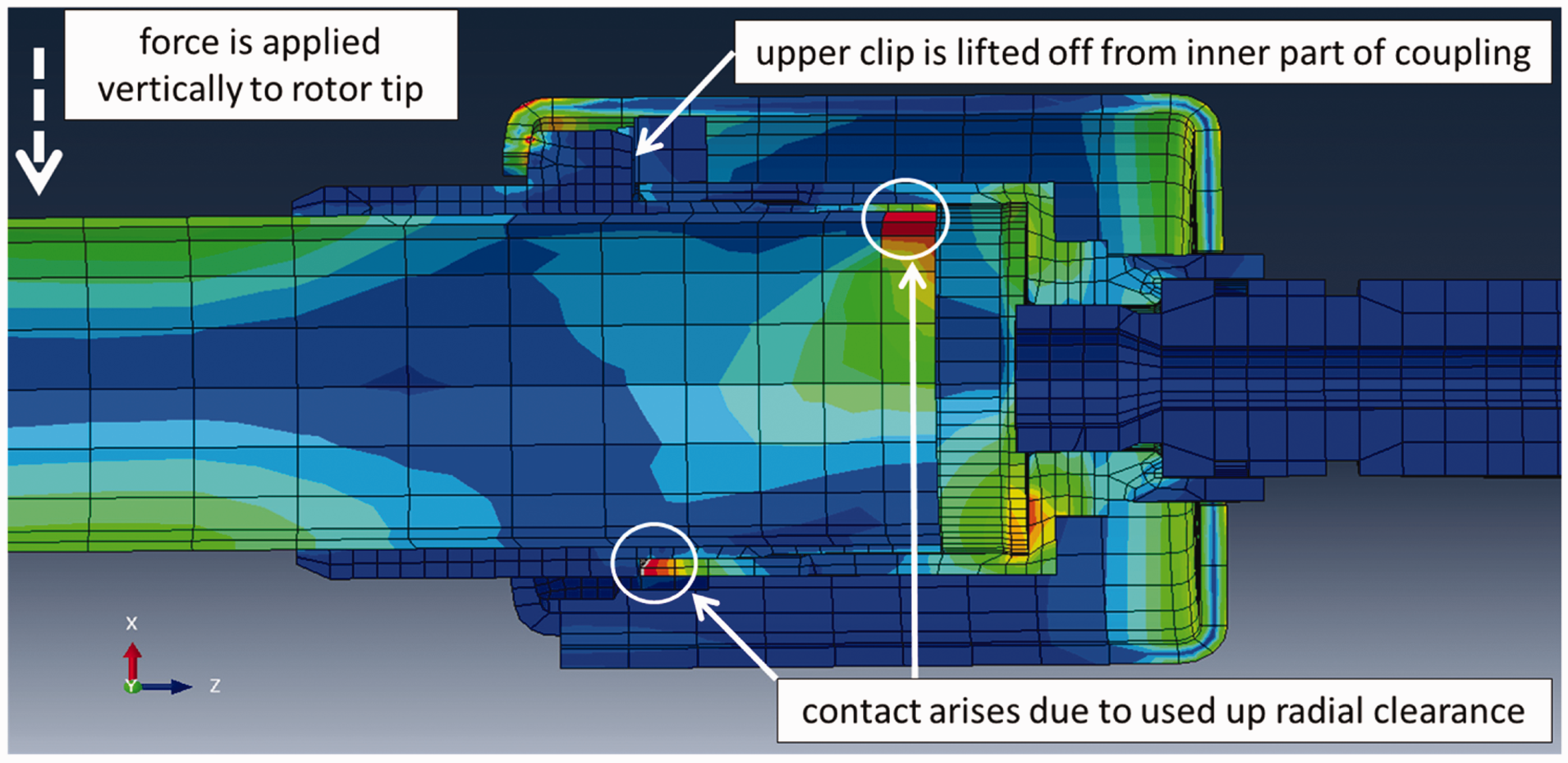
The load-displacement curve, cf. Figure 12, from the elastic simulation can be classified as “preloaded piecewise linear”. 29 The cause for the curve progression can be explained as follows: In the outlined load case, the rotor is positioned as indicated in Figure 3, lower left picture. Meaning that one pin is standing upright above the middle axis of the rotor, while the two other pins are positioned below the middle axis of the rotor; all three pins together form a tripod. If now a lateral force is applied on the rotor tip, the topmost pin is pulled away from the socket in the inner part of the coupling, therefore reducing the normal force in the contact. For the two lower pins, the opposite is the case; they are stronger pressed on the sockets of the inner coupling part. When the lateral force on the rotor tip is further increasing, at some point the axially clamping force can no longer hold the topmost pin, and it is lifted off from the socket, causing the rotor to tilt inside of the coupling. The excess of the clamping force creates the first discontinuity in the load-displacement curve in Figure 12. With a further increase of the lateral force, the tilting goes on, until the upper rear end of the rotor’s connecting end makes contact with the inner part of the coupling. As the force increases further, the rotor will slip radially (“downward”) inside of the coupling, until the radial clearance is used up and the lower front of the rotor’s connecting end makes contact with the inner piece of the coupling at the lower front area. In the load-displacement curve of the stiffened simulation, the slipping can be seen more clearly than in the elastic simulation. With even further increasing the lateral force, the rotor takes on a position as indicated in Figure 13, causing the second discontinuity. After that, the stiffness level is back to almost the same level as at the very beginning: dominated by the bending stiffness of the rotor. When computing the load-displacement curves in Figure 12, fixed boundary conditions were applied to the coupling, by doing so neglecting the compliance of the rest of system, especially that of the shaft. By taking into account the elasticity of the whole system, the discontinuities in the presented load-displacement curve will be softened significantly, depending on the stiffness relation.
It is important to notice that the difference between the stiffened and the realistic load-displacement curves in Figure 12 is not only caused by the bending stiffness of the rotor and the single components of the coupling, but is rather caused by the three dimensional interaction of the whole clamping mechanism, including slipping. This makes it hardly possible to derive a stiffness formulation without using a solid 3D FE model.
When the system is rotating, the lateral force on the rotor depends on the unbalance of the drive shaft and the excitation by the tumbling movement. If the unbalance is large enough, it might exceed the preload of the clamping spring. If this happens at a certain rotational speed, the rotor is tilting inside of the inner piece of the coupling, until the radial clearance is used up, as explained above. The tilting of the rotor increases the unbalance significantly, depending on the radial clearance. Neglecting the influence of the bending resonance, the rotor would never return to its original configuration during a run-up once the preload has been exceeded and the tilting has occurred. But with the bending resonance located within the range of the rotational speed, things are different. Once the system starts to run into the resonance, the displacement of the rotor tip will be higher than compared with the static displacement due to the unbalance force. Higher lateral displacement also means higher axial forces on the pins in the coupling. When the rotor speed is leaving the area of the resonance, the rotor displacement will decrease to its normal level. For the following experiment, the unbalance of the rotor and the preload of the coupling’s clamping spring have been carefully tuned in such a way that the preload will be exceeded when the rotor is reaching the speed of the first bending resonance. But when leaving the critical speed, the axial force on the coupling will fall below the preload of the clamping spring, allowing the coupling to “close” again.
In the experiment, the unbalance is tuned by an additional mass at the tip of the rotor. Owing to the abnormal high unbalance, the rotor displacements are much higher than in usual operation. Therefore, certain parts of the machine had to be dismounted in order to create enough space for the rotor displacements. This results in a smaller mass of the housing, causing the frequency of the bending mode to rise. The overall system behavior remains the same though.
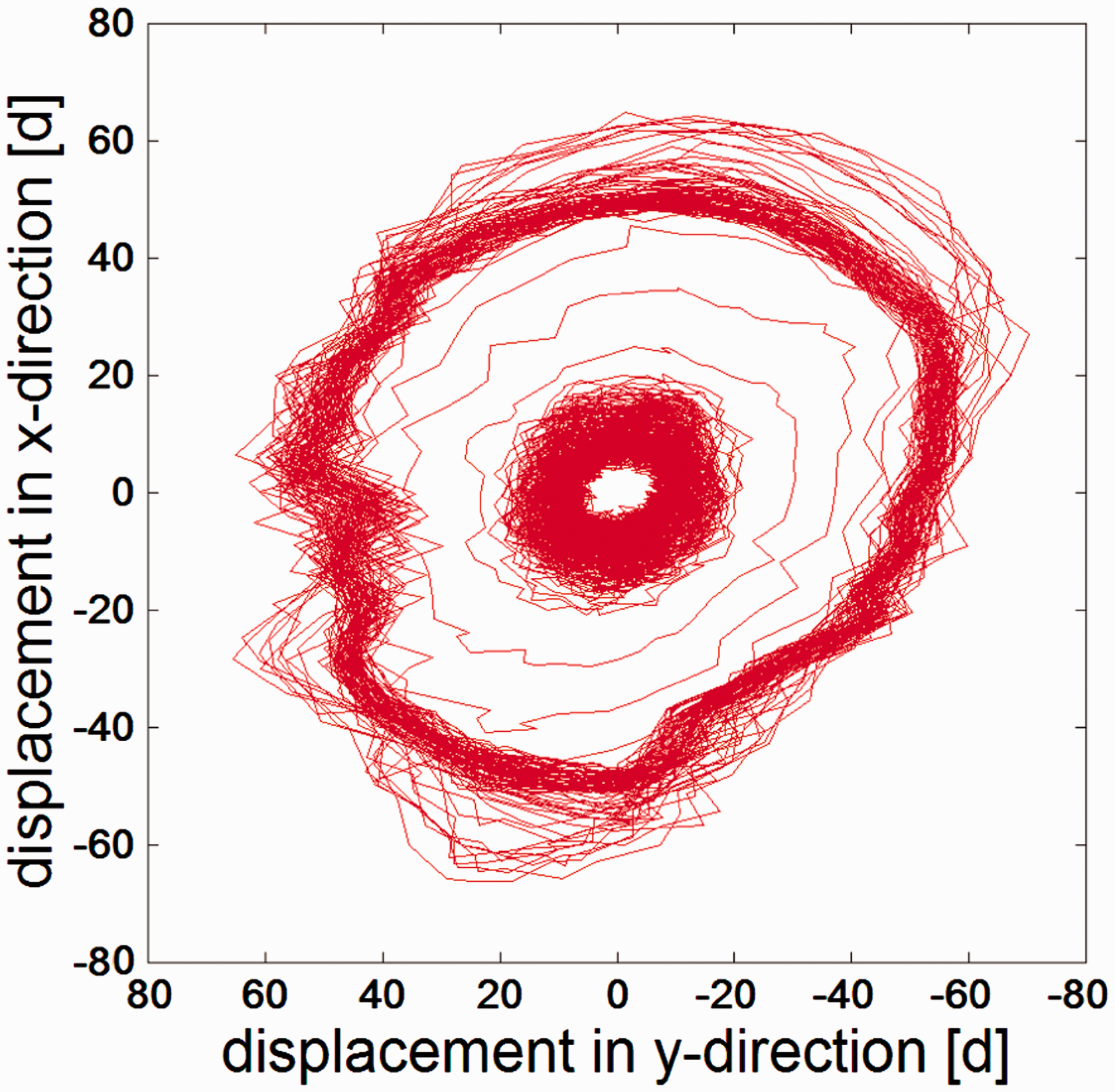
Figure 14 shows the results of the experiment by plotting the displacement of the rotor tip and the rotational speed of the drive shaft over time. The corresponding orbit plot for the time window between 9 and 11 s is presented in Figure 15.
Measurement data—vertical displacement of rotor tip relative to housing during slow run-up with additional unbalance mass at rotor tip. Measurement data—orbit plot of rotor tip, as seen from the housing looking toward the rotor.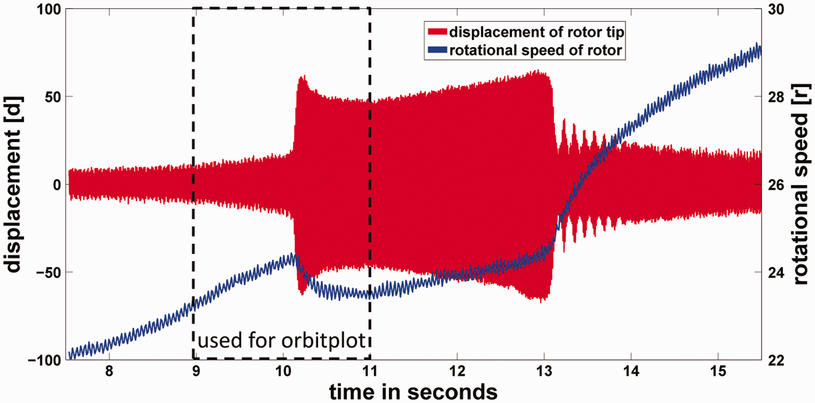
With the help of the simulation model, the data can be interpreted as follows: When the preload is exceeded at a certain rotational speed, the rotor is tilting inside of the inner piece of the coupling, until the radial clearance is used up. The discontinuity in the lateral stiffness causes a jump behavior in the lateral displacement of the rotor. Although the electric engine, which is driving the system, is relatively stiff, the rotational speed collapses significantly due to the suddenly increased moment of inertia of the rotor. Since the voltage of the electric engine is linearly increased during the run-up, the rotational speed stabilizes and starts to increase again. When the rotational speed is about to exceed the critical rotational speed, the displacement of the rotor slowly starts to decrease—and suddenly collapses when the coupling is closing again. The decreasing lateral rotor displacement leads to a decrease in the moment of inertia, causing the rotational speed to overshoot due to the principle of conservation of angular momentum. The phenomenon of the fluctuating rotational speed during the crossing of a bending resonance is known as Sommerfeld Effect 30 and is caused by a nonrigid electric engine. In the case outlined here, the Sommerfeld Effect is amplified by the opening and closing of the coupling, which leads to a sudden increase and decrease of the moment of inertia.
Right after the first “closing” of the coupling, a modulation is observed in Figure 14. The modulation frequency increases with increasing spin speed, while the amplitude is fading out. This is a very interesting phenomenon. The simulation shows that the modulation arises from a relative movement of the rotor inside of the coupling. In a coordinate system that is fixed to the coupling, the rotor is doing a backward-whirling motion. In an inertial coordinate system, the overall motion is still that of a forward whirl, which can be expected in the case of unbalance excitation. The combination of the two movements—the rotation of the coupling and the relative backward-whirling motion of the rotor within the coupling—allows the rotor to stay in resonance, even if the spin speed of the shaft is no longer matching the natural bending frequency. In other words: the mode shape is adapting to the excitation frequency to stay in resonance. This is a phenomenon which is known as mode-locking.
31
The modulation frequency matches the difference between the increasing rotation frequency and the constant whirling frequency, and is therefore also increasing. Figure 16 provides a Campbell diagram of the rotor displacement relative to the housing (measured data), showing the resonance staying on, even when the rotating speed is no longer matching the resonance frequency.
Measurement data—Campbell diagram of vertical displacement of rotor tip relative to housing during slow run-up with additional unbalance mass at rotor tip.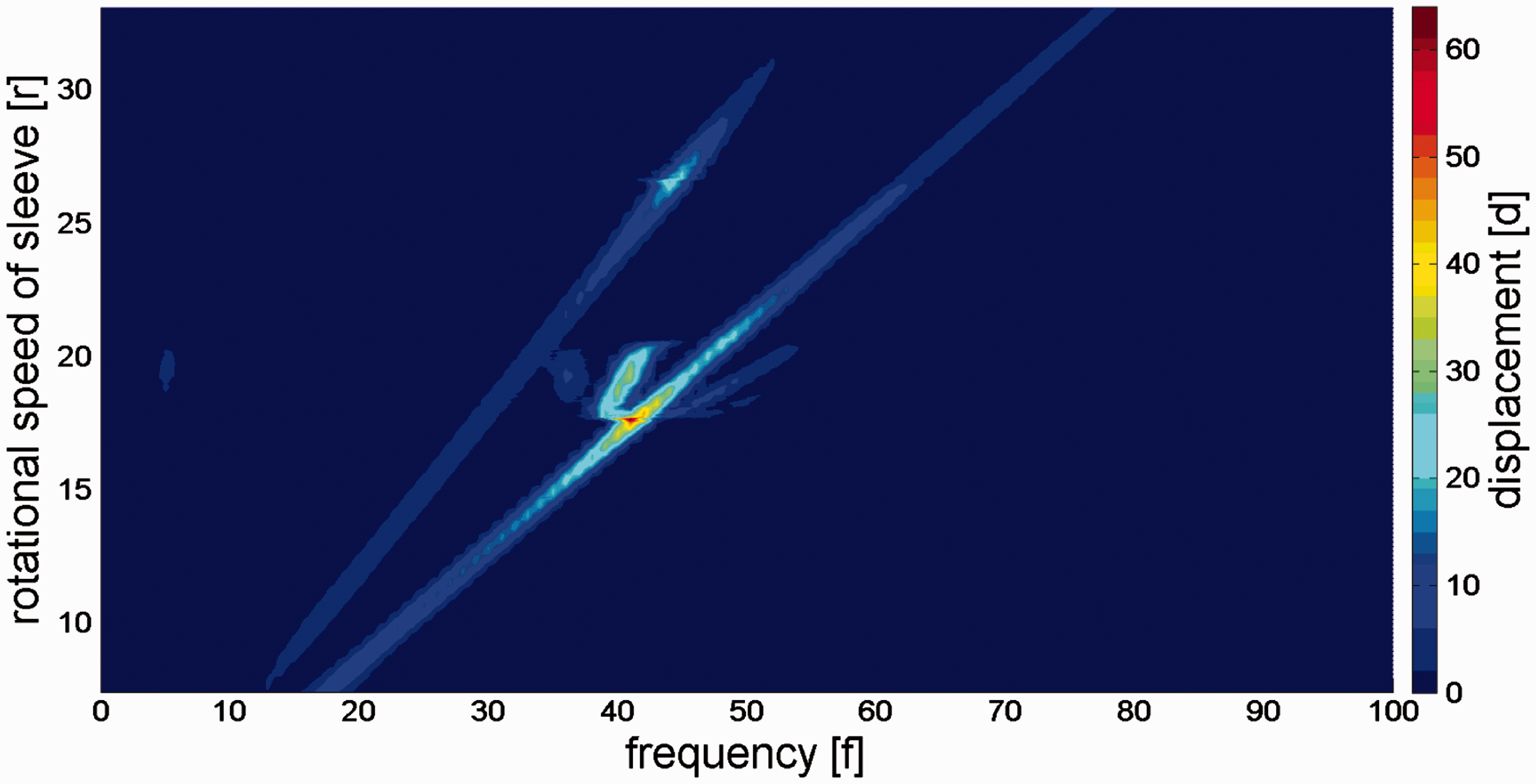
The simulation results represent the mode-locking effect well, which allows studying in detail the relative backward-whirling motion of the rotor in the coupling. An exact comparison between experiment and simulation, regarding the mentioned relative movement in the coupling, will be very difficult. It is hardly possible to place enough sensors in the rotating coupling to catch the exact movement. However, measurements at the rotor tip match well the simulation results.
Figure 17 shows simulation data corresponding to the measurements in Figure 14. There is, however, a difference between the data in the two figures: To save simulation time while still building up the model, the run-up speed in the simulation is increased compared to the one used during the measurement. Still, the simulation model represents well the effects, which can be observed in the measurements: The tilting of the rotor, when the preload of the coupling is exceeded, happens at the same rotational speed, and the modulation when running out of the critical speed due to the mode-locking effect is also present. Most likely due to the increased run-up speed, the rotor remains in resonance for a shorter period of time. The resonance amplitudes are somewhat smaller in the simulation and the Sommerfeld effect is reduced. Apart from different run-up speeds, damping could be another source for the discrepancy between simulation and measurement results. In the simulation, the tilting of the rotor does not seem to appear as abrupt as indicated by the measurement data, and may be due to an overestimated damping.
Simulation results—vertical displacement of rotor tip during run-up with additional unbalance mass at the rotor tip.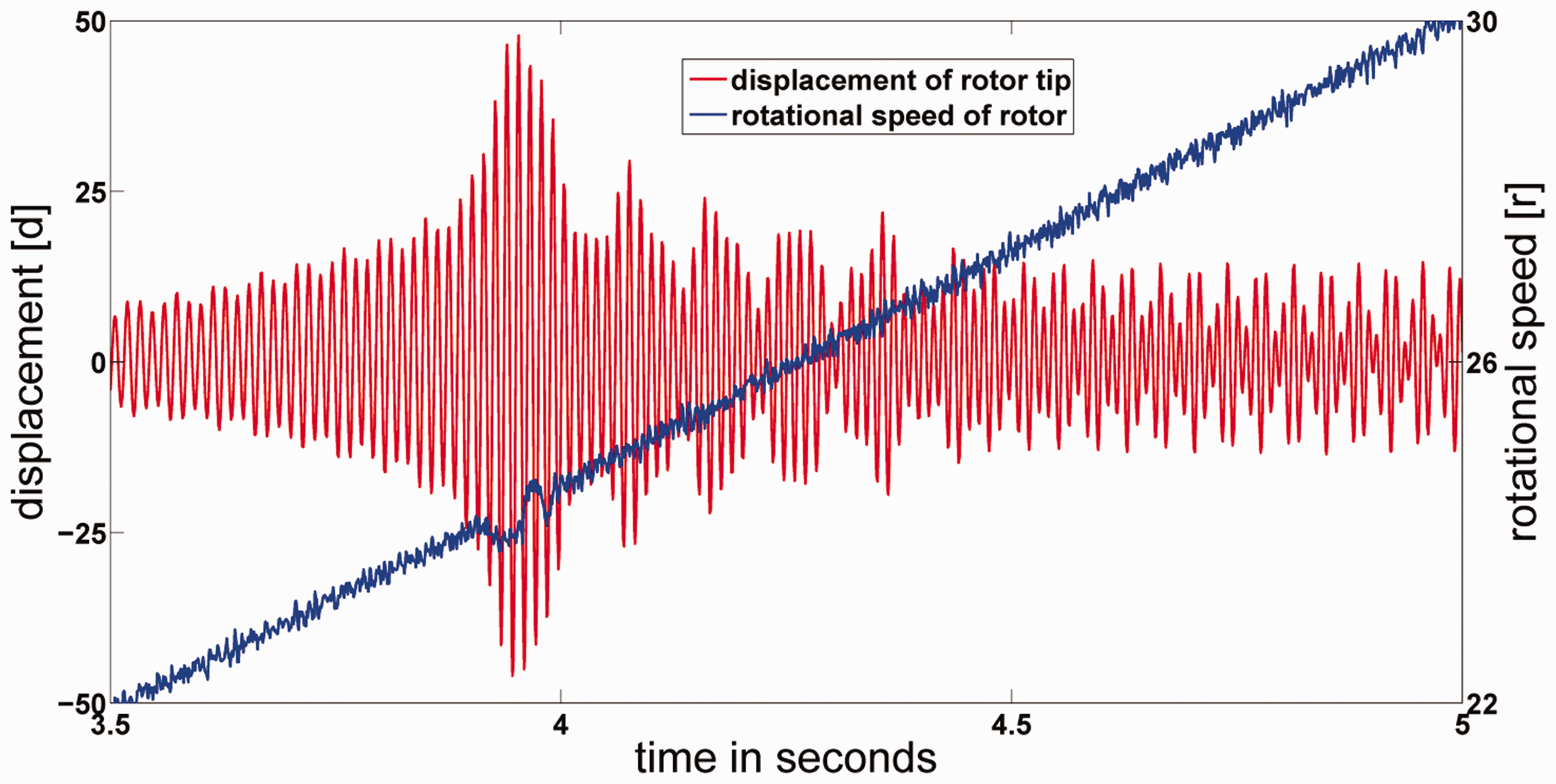
So far, additional unbalance mass at the rotor tip has been used to exceed the clamping force in the coupling. But the clamping force can be also exceeded by increasing the tumble angle ϕ of the sleeve. Figure 18 shows the corresponding results of this experiment in form of a Campbell diagram. Yet, there is an important difference compared to Figure 16. While Figure 16 shows the displacement of the rotor tip relative to the housing of the machine, the displacement in Figure 18 is measured in an absolute coordinate system. The absolute coordinate system is not chosen completely arbitrarily, but is rather the consequence of necessary changes in the support of the machine, as will be explained soon. But before that, attention shall be turned on the effect of mode-locking, which can be seen much clearer in an absolute than in a relative coordinate system. The relative backward-whirling motion of the rotor within the coupling allows the rotor system to stay in resonance, even when the excitation frequency (here: rotational speed of the sleeve) is no longer matching the natural bending frequency. This effect appears as a vertical line in the Campbell diagram of Figure 18. As the spin speed increases further, the speed of the backward whirling likewise increases—making the backward-whirling frequency the difference between the spin speed of the sleeve and the natural bending frequency.
Measurement data—Campbell diagram of vertical displacement (absolute) of rotor tip during run-up with increased tumble angle ϕ.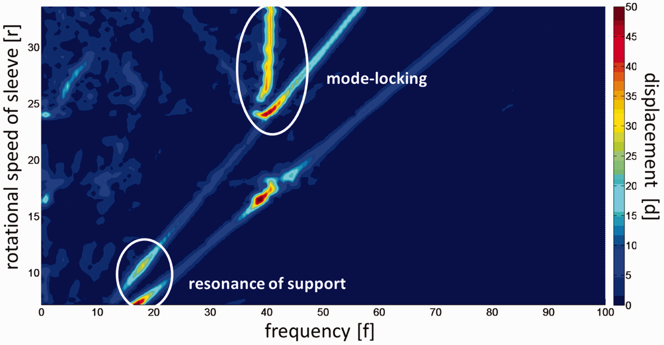
In order to be able to perform the previously described experiment, it was necessary to stiffen the supports of the machine to keep the displacement amplitudes within a reasonable range. With the new support conditions, there was no easy way to measure the relative movement between the rotor and the housing. Therefore, the displacement sensors covering the rotor movement were placed on the ground, now measuring the absolute displacement. Beside the change of the coordinate system, the new support conditions produce a noticeable resonance, which will be explained in what follows. The machine cannot be operated at a very low rotational speed, which can also be seen in Figure 7. Until now, the rigid body modes of the machine on soft supports are below the stable minimum operational speed and are therefore crossed rather fast, whereby no large resonance amplitudes occur. But with the stiffened support, the frequency of a rigid body mode lies close to the stable minimum operational speed, causing comparatively large amplitudes, which can be seen in the lower left of the Campbell diagram.
However, the structural resonances—caused by the unbalance of the rotor and by the tumbling movement—are unaffected by the changed support conditions, since they are more then two times higher in frequency.
Figure 19 shows the simulation results corresponding to the measurement data in Figure 18. The simulation requires a fast run-up at the beginning due to computational resources. Therefore, the resonance of the support does not appear in the Campbell diagram, since it is run through so fast, that it has no time to build up recognizably. Apart from that, the simulation model again represents the mode-locking effect very well. When crossing the second critical speed which is caused by the tumble excitation, the simulated resonance stays on at a higher amplitude than in the measurements, but it fades out at a lower rotational speed. Again, this might be due to an overestimated damping or due to a deviation of the friction coefficient used to model the contact between the connecting end of the rotor and the coupling.
Simulation results—Campbell diagram of vertical displacement (absolute) of rotor tip during run-up with increased tumble angle ϕ.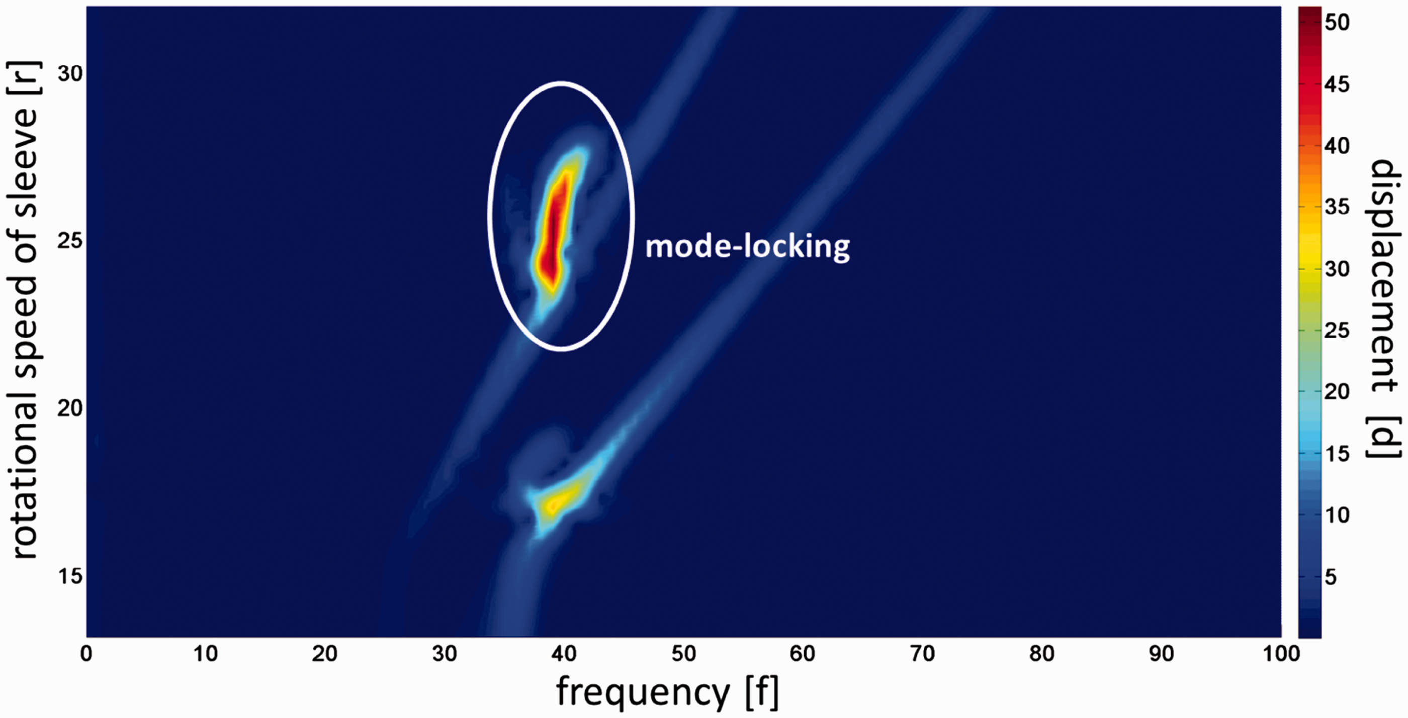
Further consistency between simulation and experiment was confirmed when certain marks at the pins of the rotor were analyzed after run-up. During the relative backward-whirling motion, the pins of the rotor are lifted off from the inner part of the coupling and returning back, according to the whirling. In doing so and according to the simulation, the pins can eventually hit the coupling during the backward whirling as indicated in Figure 20, where the edge of the rotor pin is hitting the skew surface of the coupling.
Possible contact situation between rotor and coupling during the relative backward-whirling motion.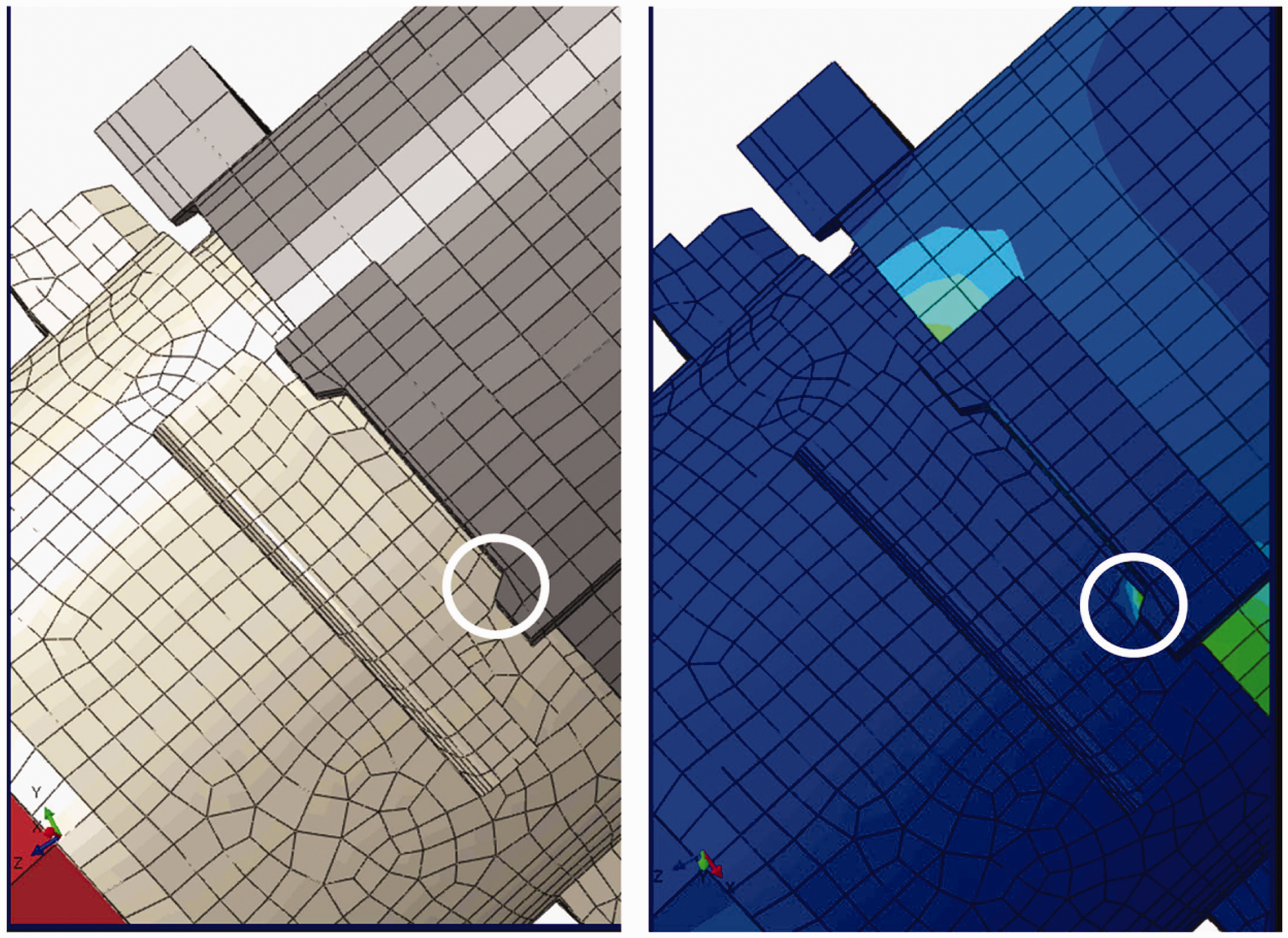
After the experiment, marks were found at the rotor pins which can only result from the described contact situation. Taken together, the simulation appears to correctly describe the overall system dynamics during the mode-locking effect.
Summary and conclusions
An example of a complex and highly nonlinear rotor system has been presented in this paper. The system cannot be simulated or even modeled accurately by using beam elements, but rather requires 3D solid modeling. This is due to the complexity and the highly nonlinear system behavior, especially with regard to the contact situation between the two-piece coupling and the rotor. ABAQUS has been used to derive an appropriate model. By doing so, the question has been addressed, whether a general purpose FEM code is able to cover the necessary rotor dynamic effects. The simulation results have been compared with measurement data, showing that the model is adequately representing the dynamic system behavior. Mode-locking resulting from nonlinear system behavior could be observed in the experiment and is well represented in the simulation model. The mathematical stability of the contact algorithm in this case is remarkable. Although the validation of the simulation model is not yet fully completed, one can state that ABAQUS—as a representative example for a general purpose FEM-code—seems to offer the modeling and computation capabilities necessary to deal with complex rotor dynamic analyses.
Footnotes
Declaration of Conflicting Interests
The author(s) declared no potential conflicts of interest with respect to the research, authorship, and/or publication of this article.
Funding
The author(s) received no financial support for the research, authorship, and/or publication of this article.