Sage Journals: Discover world-class research

Abstract

Free-form objects which have vast engineering applications are inspected using coordinate measuring machines (CMM) and non-contact scanners. The output from the devices, that is the measured point-set, must be registered with the reference profile and later inspected for the profile error. Registration is accomplished in two phases, that is coarse registration and fine registration. The most crucial step in the fine-registration stage is the profile error estimation at each point of the measured point-set. Generally, this is accomplished using the point-inversion method, which has relatively high time complexity. This work proposes a two-stage framework based on the Voronoi diagram concept for profile error estimation of 2D free-form profiles. A discretized profile is prepared for the measurement process in the first stage. The profile errors are estimated from the measured point-set using the discretized profile in the second stage. Two profile error estimation technique has been proposed based on Voronoi vertices and the Voronoi edges. The effective time-complexity of the proposed framework is O(lm log n). Implementations were executed on simulated NURBS profiles and practically measured CT-scanner data of two machined airfoils modelled as NURBS profiles. The validation results illustrate that the proposed framework’s accuracy is on par with that of the point-inversion method and is at least 56% faster than the latter; thus making it a fast and accurate alternative for CMM (operated in continuous scanning mode), CNC machine-based (in-situ) and vision-based 2D profile inspection.

Keywords

Free-form objects 2D free-form profiles Voronoi diagram NURBS profiles airfoils CT-scanner point-inversion method

Introduction

Free-form objects are objects whose surfaces cannot be categorized as planar, cylindrical or spherical surfaces. Parametric formulations like Bezier, B-spline and Non-uniform Rational B-spline (NURBS) are used to model the free-form surfaces and profiles. Due to enhanced functionality and aesthetical reasons, many aerospace, biomedical and automobile components are composed of free-form profiles and surfaces.¹ Various manufacturing operations are used for physically realizing the modelled free-form surfaces and profiles. Among them, CNC based machining process is widely used primarily for components like turbine blades² and impellers.³ Recently, Dong and Wang⁴ proposed an iterative algorithm for milling tool interference avoidance for plunge milling (rough milling operation) of impellers. Apart from this, Mali et al.⁵ gave a brief review of various aspects of free-form surface (in general) milling. The manufactured free-form surfaces and profiles will deviate from the actual surface despite precise machine tools and manufacturing devices. Hence, tolerance in both form (profile in 2D) and dimension is provided. Contact type devices like Coordinate measuring machine (CMM) and non-contact scanners are widely used to measure free-form surfaces.⁶ This work deals with profile error inspection of 2D free-form profiles measured using these devices.

CMM operates in two modes, that is discrete and continuous scanning mode. This work emphasizes the inspection of 2D profiles measured using CMM operated in continuous scanning mode or non-contact scanners. The output of the CMM or non-contact scanners will be in the form of a discrete point-set called measured point-set (M). This M needs to be compared with the reference profile (or surface in 3D) to check for tolerance conformance.

Figure 1 shows the profile tolerance specifications according to the Bureau of Indian Standards (BIS).⁷ It consists of two offset profiles separated by a distance δ which is the designer specified maximum allowable profile error. The profile error at each measured point M_i $\in M$ is given by its orthogonal distance from the reference profile (true profile). For the manufactured profile to be accepted, this profile error (at each M_i $\in M$ ) must be less than δ/2. In the case of CMM inspection, the surfaces must be sampled into sample points or scanning paths. Mian and Al-Ahmari⁸ reviewed various aspects of sampling for CMM inspection. In the case of CMM operated in continuous scanning mode, Rajamohan and Shunmugam⁹ proposed dominant isoparametric lines as CMM scanning lines. Zhou et al.¹⁰ proposed a semi-automatic path planning method for 5-axis CMM based free-form surface inspection. Later this method was improvised by Zhang et al.¹¹ Recently, Sang et al.¹² proposed a new method for generating the scanning lines for CMM inspection of free-form surfaces. However, this work deals with the profile error estimation of 2D free-form profiles measured using CMM or non-contact scanners.

Figure 1.

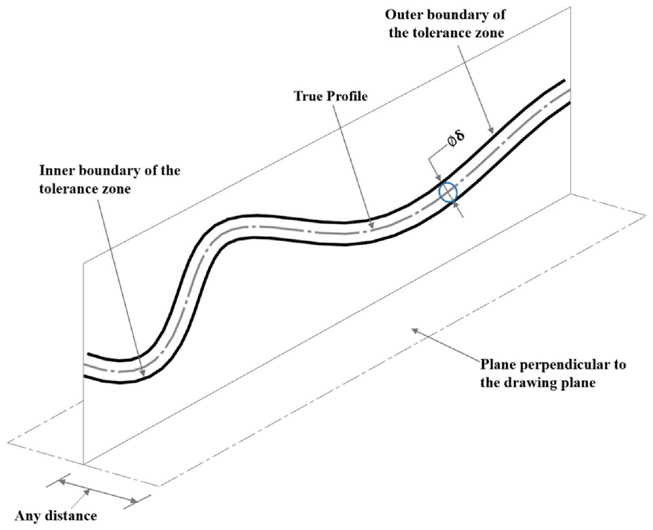
Profile tolerance zone specification according to BIS standards (Geometrical tolerancing-tolerances of form, orientation, location, and run-out).

The output of the CMM or non-contact scanners after measurement (i.e. M) needs to be aligned with the reference profile (or surface) before the profile error estimation. This process of alignment is called registration. In the presence of a datum, the alignment is with respect to it, whereas in its absence, the alignment is based directly on the free-form profile (or surface).¹ Registration is accomplished in two stages, that is, coarse and fine registration. M is initially aligned (rough alignment) with the reference profile during the coarse registration stage. In the fine registration stage, the coarsely registered M (i.e. Mc) is iteratively brought closer to the reference profile (or surface) until each of Mc_i’s (Mc_i $\in Mc$ ) profile errors is lower than δ/2. This work emphasizes profile error estimation at each Mc_i∈Mc; hence, a brief overview of various coarse and fine registration methods is presented here. In the case of CMM measurement, the coarse registration is through the traditional 3-2-1 method or customized fixtures.¹³ Apart from this, Ravishankar et al.¹⁴ proposed using a calibrated spherical gauge (CSG) for coarse registration of CMM measured data. Mehrad et al.¹⁵ proposed a four-points based method for coarse registration of M with the reference surface. In the case of CMM data, Jiang et al.¹⁶ formulated an integrated vector (based on free-form surface points) that was used to arrive at the transformation matrix needed for registration. In the case of generalized coarse registration (when there are non-contact scanners measured point-sets), Díez et al.¹⁷ reviewed various coarse registration methods. Recently Ghorbani and Khameneifar¹⁸ used Principal Component Analysis (PCA) for coarse registration of turbine blades. According to Díez et al.¹⁷, the objective function of the coarse registration stage is to reduce the Mean Square Distance (i.e. MSD) and is given by equation (1) as follows:

\begin{matrix} Meansquaredistance (MSD) \\ = \frac{1}{m} \sum_{i = 1}^{i = m} ‖ P e_{i} - ((R \times M_{i}) + t) ‖^{2} \end{matrix}

(1)

Where m is the number of points in M, R and t are the rotation and transformation matrices, and Pe_i is the nearest point to M_i in the reference profile (or surface). The Principal Component Analysis (PCA) based method is fast and useful among the coarse registration algorithm if M represents more than 95% of the manufactured profile (or surface). Hence in this work, the coarse registration algorithm used is based on PCA. The coarsely registered point-set is denoted as Mc.

In the case of fine registration, the Iterative Closest Point (ICP) algorithm proposed by Besl and McKay¹⁹ is the widely used algorithm. Brujic and Ristic²⁰ studied the effect of parameters like measurement noise, initial misalignment and the accuracy of profile error estimation on the performance of the ICP algorithm in the field of inspection. Li and Gu¹³ gave a brief overview of various fine registration techniques for the inspection of free-form surfaces. Later, Ravishankar et al.²¹ proposed the ICP based algorithm for CMM measured data. ICP algorithm is linearly convergent, and to overcome this limitation, Li et al.²² proposed an adaptive distance function (ADF) for estimating the distance between each Mc_i $\in Mc$ and the surface. Later a non-linear optimization technique was used to reduce this ADF. Xie et al.²³ proposed the minimization of the variance of the profile errors as the criteria for the convergence of the fine registration algorithm. Their method (i.e. the Variance Minimization Matching (VMM)) was theoretically found to have quadratic convergence, and they also demonstrated the same on non-contact scanner measured data.²⁴ Recently, Lv et al.²⁵ improvised the VMM based method to perform better during measurement noise presence, especially for complex surfaces. Zhu et al.²⁶ showed that heuristic methods like Genetic algorithm (GA) perform better than ICP algorithm during inspection of aero-engine blades (a typical example of a free-form object).

In all the fine registration techniques, it was observed that the profile error estimation step is essential and time-consuming. In the case of NURBS profiles, each Mc_i $\in Mc$ is projected orthogonally on the continuous profile (C(u)) using the point-inversion method to get its corresponding point (i.e. $Corres_p t_{M c_{i}}$ ) on C(u). Rajamohan et al.²⁷ used the point-inversion method explained by Piegl and Tiller.²⁸ This is an iterative method based on the Newton-raphson method. Zhang et al.²⁹ divided the NURBS surfaces into Bezier patches and projected each Mc_i $\in Mc$ on its nearest Bezier patch (using the point-inversion method) to find its profile error (or form error). Ko and Sakkalis³⁰ gave a brief overview of various geometric based methods (i.e. geometric iterative algorithms) to reduce the execution time of the point-inversion method. Recently, Li et al.³¹ proposed a normal-curvature-based method to accelerate the point-inversion method.

Apart from the point-inversion method, Lang et al.³² and He et al.³³ used the subdivision based method (in the parametric domain). Similar to this method, Liu³⁴ proposed the usage of linear quadtree based for estimating the $Corres_p t_{M c_{i}}$ for each Mc_i $\in Mc$ . Biradar and Pande³⁵ used the reference surface’s tessellated (i.e. triangulated) representation. Similarly, Lang et al.³² used the reference surface’s stereolithography (STL) model. Instead of triangulated representation, Ravishankar et al.²¹ proposed the quadrilateral facet method for form error estimation.

Among all the above methods, the point-inversion method is the most accurate. However, it executes in O(ms) time for m measured points. The value of s depends on the number of iterations, which depends on the user-defined convergence criteria. A lower convergence criterion increases the accuracy and the number of iterations. The geometric algorithms reviewed by Ko and Sakkalis³⁰ accelerate the convergence of the point-inversion method. However, they are iterative. The surface subdivision method is similar to that of the point-inversion method. Tessellated representations, STL models and quadrilateral facets are discrete representations of the free-form profiles (and surfaces). However, there always exists a trade-off between the point density and the profile error estimation accuracy in this case. Hence, a discretization strategy and profile error estimation technique (with at least logarithmic time-complexity) from the discretized profile (especially 2D profiles) is needed.

The algorithms of most of the computational geometric techniques have logarithmic time-complexities and are promising. Techniques like the Voronoi diagram and its dual, that is the Delaunay triangulation, are used for curve and surface reconstruction.³⁶ Samuel and Shunmugam³⁷ proposed using the farthest-point Voronoi diagram to estimate circularity. OuYang et al.³⁸ developed a coarse registration technique (for point clouds) based on the concept of Delaunay Pole Spheres (DPS). This DPS is based on the poles concept proposed by Amenta and Bern³⁹ for surface reconstruction. Amenta and Kolluri⁴⁰ and Amenta et al.⁴¹ theoretically proved that for a dense sampling, the pole spheres approximate the surface. Based on this fact, Hari Ganesh and Samuel⁴² developed a method for form error estimation of free-form surfaces. The theoretical proof of Amenta et al.⁴¹ holds true even in the case of 2D profiles, and the 2D pole circles approximate the continuous profile.

Moreover, the 2D Voronoi diagram has O(n log n) time-complexity, unlike the 3D Voronoi diagram (i.e. O(n²log n) time-complexity). Hence, the 2D Voronoi diagram is used in this proposed work. The method proposed by Hari Ganesh and Samuel⁴² is dedicated to CMM operated in discrete scanning mode. A more generalized method, primarily for CMM operated in continuous scanning mode, and non-contact scanners are needed. In this direction, the contribution of this work is as follows:

A new method for discretizing the 2D reference free-form profiles (especially for profile error inspection).

Techniques for fast and accurate estimation of profile errors at each Mc_i $\in Mc$ using the discretized profile.

The rest of the paper is organized as follows: Section 2 describes the Voronoi diagram and the associated theoretical details used in this work. Section 3 describes the algorithms of the proposed framework. Section 4 explains the proposed framework’s practical implementations, and section 5 concludes the paper.

Preliminaries

Voronoi diagram and poles

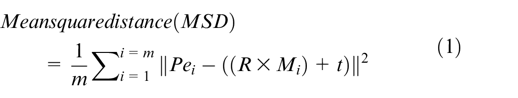
For a set of points P in $R^{d}$ , the nearest point Voronoi diagram divides the space into regions called Voronoi cells enclosing each P_i $\in P$ and bounded by hyperplanes. In the case point-set Pe in $R^{2}$ (i.e. 2D), the hyperplanes are Voronoi edges which are the equi-distant line between any two points [Pe_i, Pe_j]i≠j. The intersection points of the Voronoi edges are the Voronoi vertices (Figure 2(a)). As observed in Figure 2(a), the Voronoi cells of Pe_i’s lying on the convex hull of Pe is open, whereas those not lying on the convex hull of Pe is closed.

Figure 2.

Voronoi diagram, poles and profile error estimation: (a) Voronoi diagram of a point-set Pe, (b) Voronoi cell and Poles of Pe_i, (c) Profile error estimation using max.pole circle, and (d). Profile error estimation using min. pole circle.

Poles are extreme Voronoi vertices of a Voronoi cell. Amenta and Bern introduced this concept.³⁹ Consider the Voronoi cell of a point Pe_i $\in Pe$ (i.e. V(Pe_i)). Since this point is not on the convex hull of Pe, V(Pe_i) is closed (Figure 2(b)). Among the Voronoi vertices of V(Pe_i), $υ_{2}$ is farthest from Pe_i, and hence it is chosen as the maximum pole of Pe_i (i.e. $Max . Pol e_{P e_{i}}$ ). Among, the remaining Voronoi vertices of V(Pe_i), $∠ υ_{2} P e_{i} υ_{5}$ is maximum. Hence, $υ_{5}$ is considered as the minimum pole of Pe_i (i.e. $Min . Pol e_{P e_{i}}$ ). This angle is considered as the pole angle at Pe_i (i.e. θ).

Pole circles and profile error estimation

In the case of the nearest point Voronoi diagram, the poles of a point Pe_i are centres of empty circles that pass through it. Amenta et al.⁴¹ have theoretically proved that in the case of dense 3D point-sets (following the ε-sampling criteria), the poles approximate the medial axis and the pole spheres approximate the surface from which the 3D point-set is sampled. However, in the case of 2D, all the Voronoi vertices (including the poles) approximate the medial axis and the pole circles the continuous Profile C(u) from which Pe is discretized. This theoretical concept is used in this work. Consider a measured point Mc_i $\in Mc$ and let Pe_i be its nearest point in Pe. The profile error can be approximated using the Max. Pole circle (Figure 2(c)) and the Min. Pole circle (Figure 2(d)) of Pe_i and the equations are as follows:

e_{1} = r_{\max} - ‖ Max . Pol e_{P e_{i}} - M c_{i} ‖

(2)

e_{2} = r_{\min} - ‖ Min . Pol e_{P e_{i}} - M c_{i} ‖

(3)

e_{P_M c_{i}} = \max (| e_{1} |, | e_{2} |)

(4)

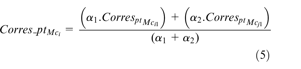
Where r_max (in equation (2)) is the radius of the Max. Pole circle and r_min (in equation (3)) is the radius of the Min. pole circle. The profile error is represented by $e_{P_M c_{i}}$ (equation (4)) and only the absolute value of $e_{1}$ and $e_{2}$ is considered in this work.

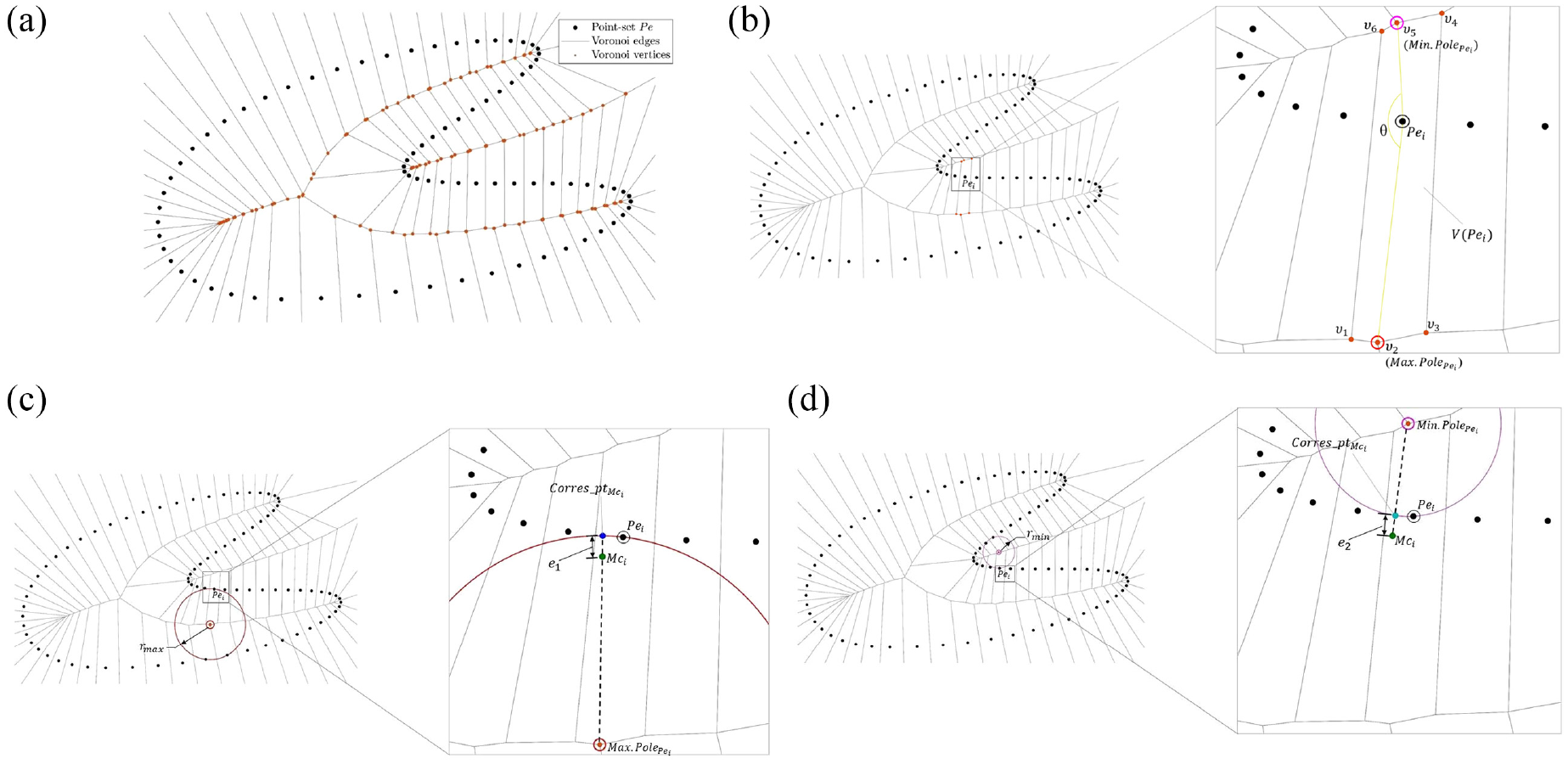
The corresponding point of Mc_i on C(u) is approximated by projecting it on both the pole circles of Pe_i (shown as $Corres_p t_{M c_{i}}$ in Figure 2(c) and (d)). Depending upon the maximum values of $e_{1}$ and $e_{2}$ , the appropriate $Corres_p t_{M c_{i}}$ is chosen as the approximate point of projection (i.e. the corresponding point) of Mc_i on C(u). Since Mc_i is projected on the pole circles, the order of approximation of profile error is two. Since each Mc_i is projected on the pole circles, this technique is also called Poles Circles Project (PCP) technique.

Voronoi edge assisted weighing (VEAW)

In the case of a continuous profile, the projection point of the measured point Mc_i $\in Mc$ on C(u) lies in the vicinity of its nearest point in Pe (i.e. Pe_i). This projection point (or the corresponding point) can be approximated using interpolation in the discrete case. For this purpose, the two nearest points of Mc_i are considered (i.e. Pe_i and Pe_j, Figure 3). The Voronoi vertices of the edge E_ij (represented by the line segment $\underline{υ_{1} υ_{2}}$ ) between Pe_i and Pe_j is used for computing the angular weights ( $α_{1}$ and $α_{2}$ ) and it is graphically depicted in Figure 3.

Figure 3.

Angular weights computation using the Voronoi edge.

As shown in Figure 3, $υ_{1}$ is farthest from both Pe_i and Pe_j. Hence it is considered for angular weights computation. The approximate projection point of Mc_i on C(u) (i.e. $Corres_p t_{M c_{i}}$ ) (equation (5)) and the corresponding profile error (i.e. $e_{P_M c_{i}}$ ) (equation (6)) is estimated as follows:

Corres_p t_{M c_{i}} = \frac{(α_{1} . Corre {s_{pt}}_{M c_{i 1}}) + (α_{2} . Corre {s_{pt}}_{M c_{j 1}})}{(α_{1} + α_{2})}

(5)

e_{P_M c_{i}} = ‖ Corres_p t_{M c_{i}} - M c_{i} ‖

(6)

Where, $Corre {s_{pt}}_{M c_{i 1}}$ is the projection of Mc_i on the Max. Pole circle of Pe_i and $Corre {s_{pt}}_{M c_{j 1}}$ is the projection of Mc_i on the Max. Pole circle of Pe_j. Since Pe_i is relatively near to Mc_i, higher weight (i.e. $α_{1}$ ) is considered for Pe_i. This proposed formulation (i.e. equation (5)) is similar to the Lagranges first-order interpolation. Since the Max. Pole circles of Pe_i and Pe_j are considered in equation (5); the order of approximation of the profile error (equation (6)) is two.

Oriented Bounding-box (OBB)

This geometrical entity is a rectangle that encloses all the points of Pe. This box is computed through PCA of Pe. The computed OBB consists of four corner points. Initially, the covariance matrix of Pe (i.e. Cov(Pe)) is calculated using equation (7) as given by Chung et al.⁴³

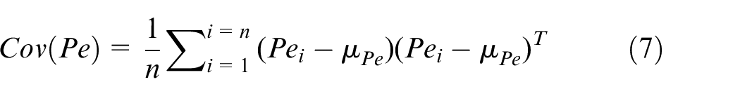
Cov (Pe) = \frac{1}{n} \sum_{i = 1}^{i = n} (P e_{i} - μ_{Pe}) {(P e_{i} - μ_{Pe})}^{T}

(7)

Where n is the number of points in Pe and $μ_{Pe}$ is the mean-coordinate of Pe. Later the eigenvectors ( $υ_{1}$ and $υ_{2}$ ) are obtained through eigendecomposition of Cov(Pe). The sides of OBB are parallel to the eigenvectors.

Methodology

As shown in Figure 4, the proposed methodology consists of two stages. Before developing the methodology, the following assumptions are made:

The profile has a well-defined parametric formulation and does not have any self-intersections.

The profile is at least C2 continuous without straight portions and sharp corners (except at the starting and ending points).

The measured point-set is outlier free and represents at least 98% of the reference profile.

The measured point-set is dense enough (at least 500 points) and is distributed evenly throughout the profile.

Figure 4.

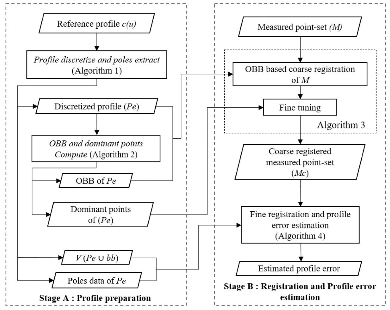
The schematic of the proposed framework.

In stage A, initially, the profile is discretized, and the poles data for each discrete point is extracted using the profile-discretize and poles extract algorithm. Later, PCA based oriented bounding-box (OBB) and the dominant-points of Pe are computed. This stage can be implemented apriori to the measurement process, and hence it is not part of the actual inspection cycle. The discretized Profile (Pe), its OBB, and the dominant-points are used for initial coarse registration and fine-tuning of the measured point-set (M) with Pe in stage B. Later in the same stage, the Voronoi diagram and poles data of Pe is used in the profile error based fine registration algorithm for fine registration of Mc with Pe.

Profile-discretize and poles extract

This Voronoi diagram-based algorithm is used to arrive at the discretized Profile (Pe) and its corresponding poles data. As shown in Supplemental Figure 1, an arbitrarily discretized profile (P) is given as input in this algorithm. A limit for pole angle (θ_max) and minimum step value (in the parametric domain (Δm) is set (Step 1 and 2 of Supplemental Figure 1). Initially, P is enclosed in an arbitrary box (bb) (Step 4) to avoid infinite Voronoi vertices. Later, the point-density of P is increased iteratively (Steps 5–9) until all the pole angles corresponding to each P_i $\in P$ are above θ_max. The poles.extract function (Step 6) and the nurbs.pt.calculate are MATLAB functions written by the authors – the former extracts the poles data from the V(P $\cup bb$ ). The latter is used for discretizing the profile and is based on the NURBS formulation given by Piegl and Tiller.²⁸ The outputs of this algorithm are, discretized Profile (Pe) (having n points) and the Voronoi diagram of $Pe \cup$ bb (i.e. V( $Pe \cup$ bb)). Supplemental Figure 2 shows the graphical representation of this algorithm.

Oriented Bounding Box(OBB) and Dominant points compute

In this algorithm (Supplemental Figure 3), the OBB of Pe (Supplemental Figure 4(a))is computed using the PCA of Pe as explained in the previous section (i.e. Oriented Bounding Box (OBB)). The eigenvectors of Cov(Pe) is considered as Pe’s local reference frame (LRF) (Supplemental Figure 4(b)), and the mean coordinate of Pe (i.e. µ_e) is chosen as the origin of the LRF (Step 2, Supplemental Figure 3). The computed OBB (Supplemental Figure 4(c)) consists of the coordinates of the four corner points of OBB. The local coordinates of Pe (i.e. Loc.Pe) are calculated using the considered LRF. Later, the absolute curvature Kc_i $\in Kc$ of each Pe_i $\in Pe$ is computed using the formulation given by Liu et al.⁴⁴ The dominant points (i.e. Pe_dom) are selected from Pe based on the Kc values (Steps 3–7) (Supplemental Figure 4(d)). The local coordinates (Loc.Pe_dom) corresponding to each Pe_dom are chosen from Loc.Pe.

Coarse registration and fine-tuning

In this algorithm (Supplemental Figure 5), the OBB of the measured point-set (M) is initially calculated using the eigenvectors obtained through M’s PCA (Step 1, Supplemental Figure 5) (Supplemental Figure 6(b)). M is coarsely registered with Pe by aligning the OBB of M with that of Pe (Step 2) (Supplemental Figure 6(c)). To avoid the flipping of M, the alignment is brought by considering the diagonal points of both the OBB. The local coordinates of measured points after coarse registration (i.e. Mco) are computed (i.e. Loc.Mco) (Step 3, Supplemental Figure 5). The indices of the nearest points in Loc.Mco for each point in Loc.Pe_dom is found. Later, the points in Mco corresponding to those indices are used for transforming Mco to Mc (closer to Pe) (Steps 4 and 5, Supplemental Figure 5) (Supplemental Figure 6(d)). This transformation process constitutes the fine-tuning part after coarse registration.

Fine registration and profile error estimation

This algorithm is used for profile error estimation at each Mc_i $\in Mc$ . In this algorithm, Mc is iteratively moved closer to Pe so that the profile error of the measured component reduces. As mentioned in Supplemental Figure 7, this algorithm consists of a nested loop. In the outer while loop, the Transformation of Mc is accomplished using the ICP method of Besl and McKay. In the inner for loop, the profile error at each Mc_i $\in Mc$ (i.e. $e_{P_M c_{i}}$ ) and its corresponding point on the profile (i.e. Corres_pt_Mc(i)) is computed (Steps 4 and 5, Supplemental Figure 7). The pole-circle-projection-(PCP) technique or the Voronoi edge assisted weighing (VEAW) technique is used in the profile. Error.Estimate function. The computed Corres_pt_Mc is used to transform Mc (Steps 10 and 11) during each iteration. The value of maximum profile error (i.e. $e_{P_\max}$ ) (Step 7) is the estimated profile error during each iteration. The authors defined ‘Transformation. Compute’ function uses the quaternion based method proposed in the ICP algorithm. The outer loop iteration stops if either of the three conditions (mentioned in Steps 1, 2 and 3) is achieved. The final value of $e_{P_\max}$ is the profile error of the measured component.

Time-complexity

The profile discretize and poles extract algorithm (algorithm 1) is based on the concept of the 2D Voronoi diagram, which has O(n log n) time-complexity.⁴⁵ The Voronoi diagram and the associated poles in this algorithm is computed for each iteration. Moreover, the value of n increases as this algorithm is executed. The OBB and dominant points compute algorithm (algorithm 2) is based on the PCA technique and discrete curvature computation method and executes is O(n) time.

Among the techniques used in the coarse registration and fine-tuning algorithm (algorithm 3), the nearest neighbour search technique (based on the Voronoi diagram) executes in O(m log n) time for m number of points in Mc and n number of points in Pe. Moreover, the OBB based coarse registration and the dominant-points based fine-tuning method executes in O(m) time. In the case of the fine registration and profile error estimation (algorithm 4), the nearest neighbour search technique executes in O(m log n) time for each iteration and the Transformation. Compute’ function executes in O(m) time. As this section’s beginning says, stage A (consisting of the first two algorithms) can be completed apriori and does not form part of the measurement process. Hence the effective time-complexity is O(m log n) for algorithm3 and O(lm log n) for algorithm 4(for l iterations of the outer while loop).

Implementation and its results

The proposed two-stage methodology algorithms were programmed using MATLAB 2018a software in a PC with Intel © Core™ i5 3.0GHz(4cores) processor with 31.9 GB RAM. Implementations were executed for simulated profiles and practically measured data obtained by measuring two machined profiles.

Implementations for simulated profiles

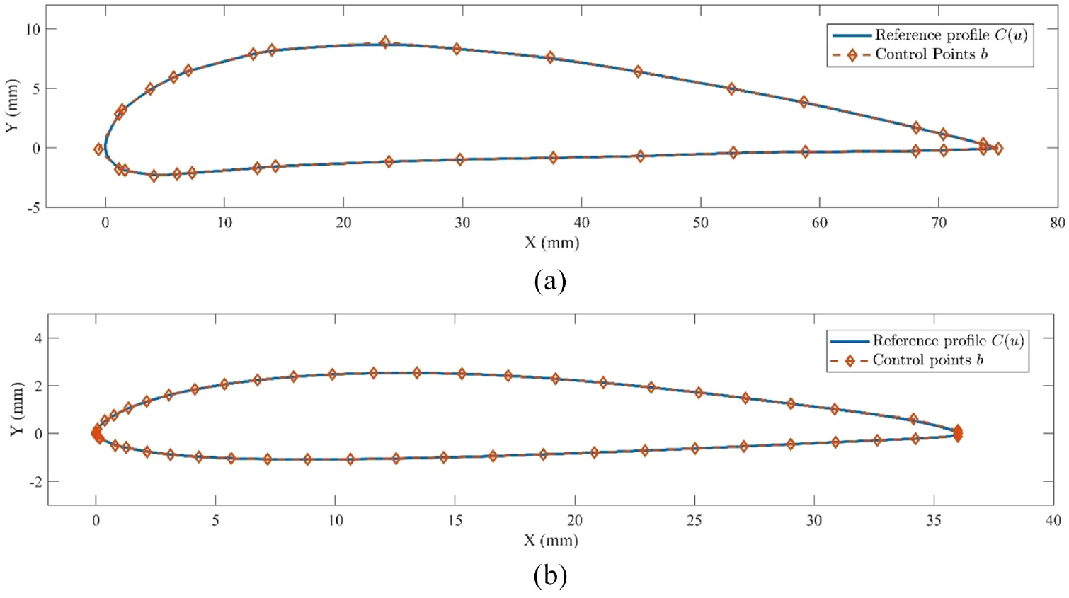
Two open profiles and one closed profile are modelled using the NURBS formulation. Figure 5(a) to (c) show the control points and the corresponding profiles. The degree of the profiles is chosen as 2, 3 and 4, respectively. Supplemental Tables 1, 2 and 3 give the coordinates of the control points of the profiles.

Figure 5.

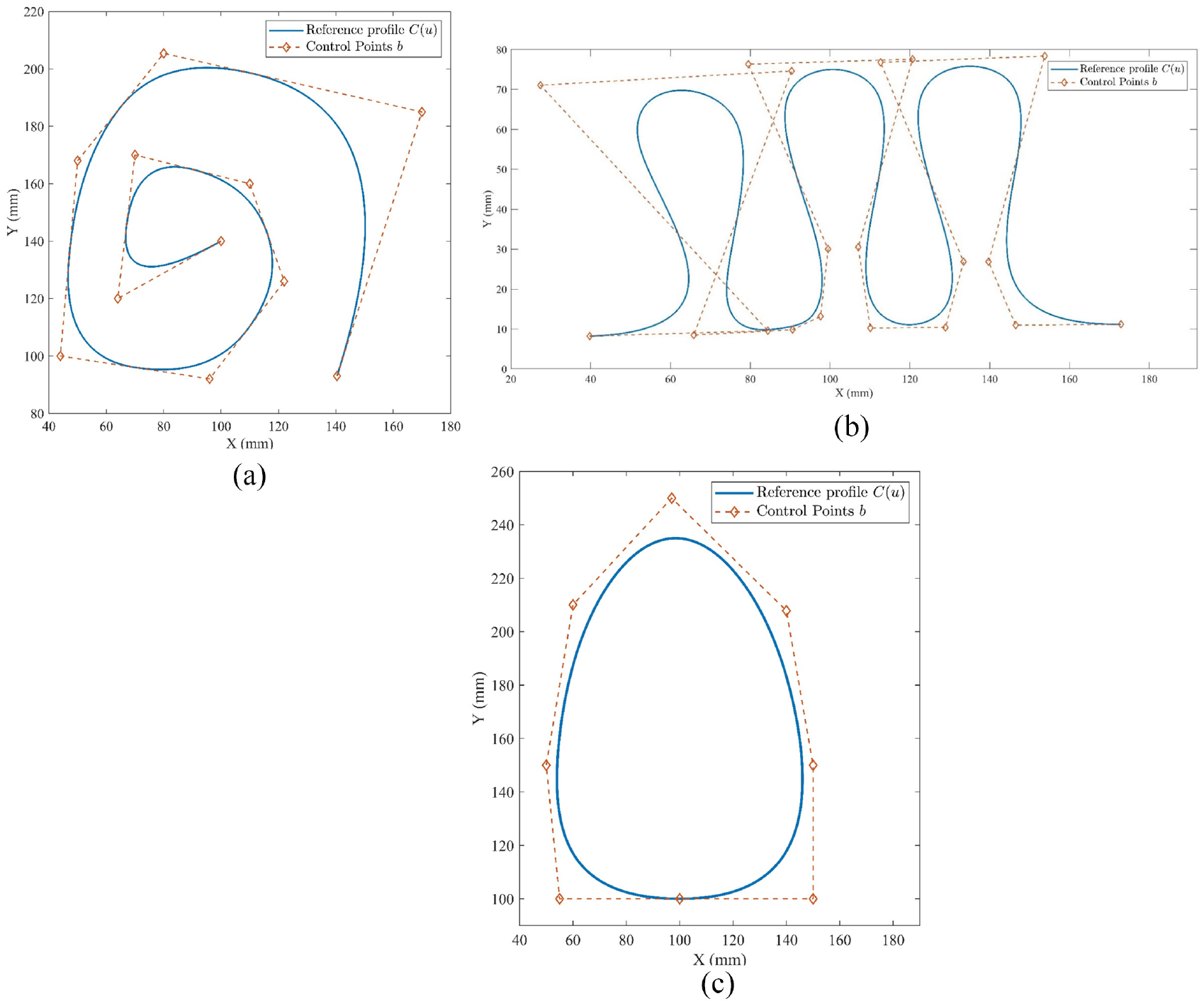
Free-form profiles considered for implementations: (a) Free-form profile 1, (b) Free-form profile 2, and (c) Free-form profile 3.

Profile discretize and poles extract algorithm (algorithm 1) is implemented for all the three reference profiles to get their respective Pe’s (i.e. Pe_P1, Pe_P2 and Pe_P3). The minimum step size (i.e. Δm in the parametric domain) of 10⁻⁴ and the minimum pole angle (i.e. θmin) of 178° is considered during the implementation. The number of points (i.e. n) in the three Pe’s was 10,000. Later, the OBB and the dominant points for the Pe’s were computed using the OBB and dominant points compute algorithm (algorithm 2).

Simulation of measured profiles

During the manufacturing processes, errors are bound to occur due to which the manufactured profiles deviate from the reference profile. Apart from this, errors also add up during the measurement process. In the case of free-form profiles, these errors are classified as profile errors and random errors. Similar to the authors’ previous work,⁴² in this work, the profile errors and random errors are simulated as follows:

Inducing profile errors: The control points (b) of the profile are perturbed by adding random numbers to get a new set of points (b_per). Later, a new discrete profile (D_per) is generated using b_per. For the free-form profiles mentioned previously, the control points of each of the profiles are perturbed by adding random numbers having 0 mean and 0.05 mm standard deviation. Later three D_per’s (i.e. D_{per_P1}, D_{per_P2} and D_{per_P3}) having 1000, 1250 and 2000 points (respectively) are generated using their respective b_per’s.

Inducing random errors: Each point of D_per is randomly perturbed (along its normal direction). For each the three D_per’s, corresponding random number arrays (having 0 mean and 0.01 mm standard deviation and following Gaussian distribution) is generated. Each random number arrays have 1000, 1250 and 2000 random numbers corresponding to D_{per_P1}, D_{per_P2} and D_{per_P3}, respectively. Later the D_per_s are perturbed by their corresponding random number arrays.

Furthermore, D_{per_P1} is rotated by 124°, D_{per_P2} is rotated by 92°, and D_{per_P3} is rotated by 82° (all in the anti-clockwise direction) to get three sets of simulated measured point-sets (M).

Coarse registration and profile error estimation

The simulated measured point-sets (i.e. M’s) are roughly aligned with their corresponding Pe’s using the Coarse registration and fine-tuning algorithm (algorithm 3) to get their corresponding coarsely registered measured point-sets (i.e. Mc). Figure 6 shows the results of the implementation of algorithm 3 for simulated profiles, whereas Table 1 shows the reduction in the MSD values after coarse registration.

Figure 6.

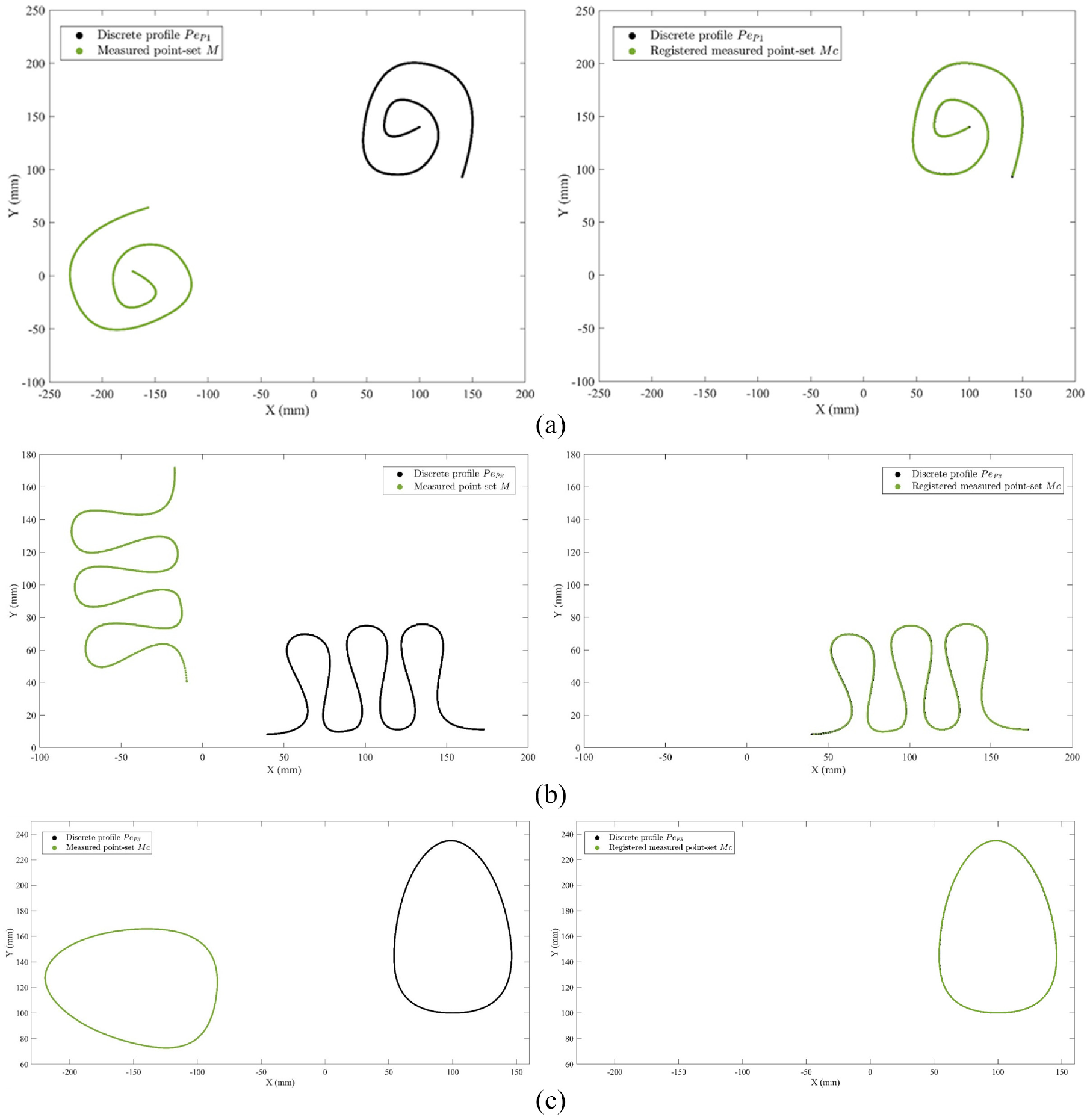
Implementation of Coarse registration and fine-tuning algorithm for simulated profiles (algorithm 3): (a) Free-form profile 1, (b) Free-form profile 2 and (c) Free-form profile 3.

Table 1.

Implementation results of stage B of the methodology for simulated profiles θmin = 178°, $Δ$ m = 10⁻⁴.

Profile and degree	No. of points in Mc (m)	Coarse registration and fine-tuning (Mean. Sq. distance) (mm²)		Fine registration and profile error estimation			Absolute deviation (µm)		Gain in accuracy (%)
Profile and degree	No. of points in Mc (m)	Before	After	$e_{P_\max_PI}$ (mm)	$e_{P_\max_PCP}$ (mm)	$e_{P_\max_VEAW}$ (mm)	$d_{ab s_{PCP}}$	$d_{ab s_{VEAW}}$	Gain in accuracy (%)
n = 10,000
Profile 1 (Degree = 2)	1000	6.49 × 10⁴	0.0107	0.073475	0.073459	0.073464	0.016	0.011	31.25
Profile 2 (Degree = 3)	1250	1.19 × 10⁴	0.0082	0.094486	0.094508	0.0944856	0.02	4×10^-4	98.00
Profile 3 (Degree = 4)	2000	4.81 × 10⁴	0.0040	0.090606	0.090602	0.090607	0.004	0.001	75.0

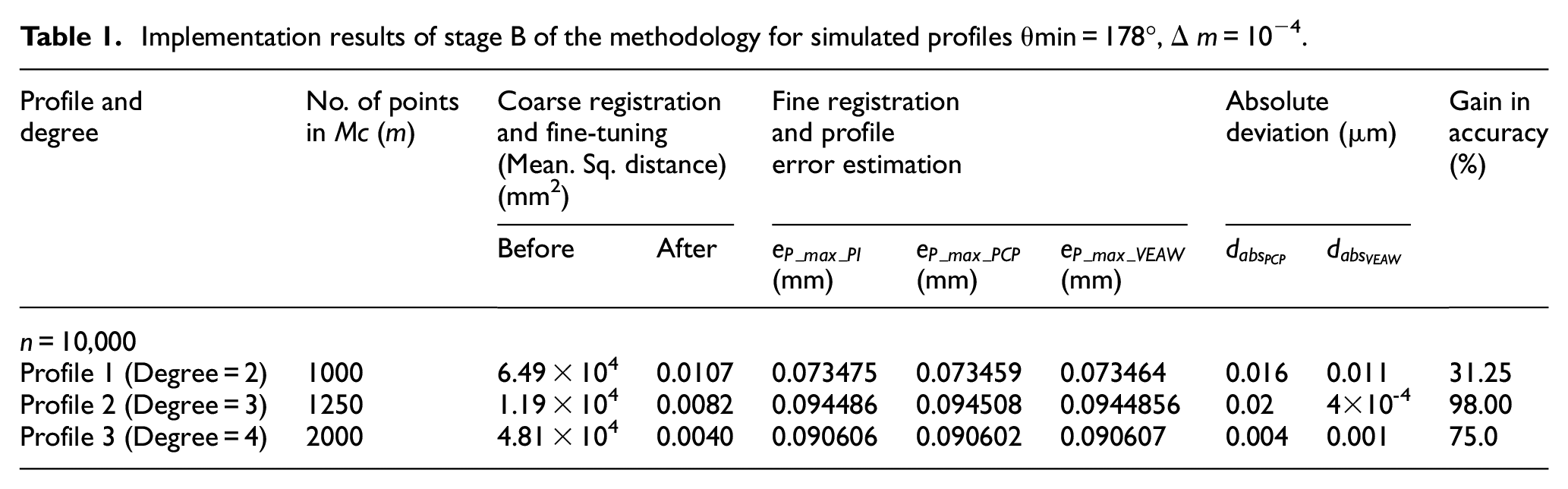
After implementing algorithm 3, each of the Mc’s (corresponding to free-form profiles 1, 2 and 3) are fine registered with Pe_P1, Pe_P2 and Pe_P3 using the Fine registration and profile error estimation algorithm (algorithm 4). During each iteration of algorithm 4 (ICP based method), the profile error and the corresponding point-set, respectively (containing the projection of Mc_i on C(u)), were estimated using both PCP ( $e_{P_\max_PCP}$ , $Corres_p t_{Mc_PCP}$ ) and VEAW ( $e_{P_\max_VEAW}$ , $Corres_p t_{Mc_VEAW}$ ) techniques.

Later the values of both $e_{P_\max_PCP}$ and $e_{P_\max_VEAW}$ are validated using the point–inversion method (i.e. using it in the inner for loop of algorithm4). A cosine error of 10⁻⁶ is considered for each Mc_i $\in Mc$ to ensure an accurate orthogonal projection of Mc_i on C(u). The absolute deviation (d_abs) between $e_{P_\max_PI}$ , $e_{P_\max_PCP}$ (i.e. $d_{ab s_{PCP}}$ ) and $e_{P_\max_PI}$ , $e_{P_\max_VEAW}$ (i.e. $d_{ab s_{VEAW}}$ ) is calculated. Supplemental Figure 8 depicts the convergence plots of the fine registration and profile error estimate algorithm (algorithm 4) for the Mc’s corresponding to all the three profiles. The execution time per iteration (i.e. ET/iter of algorithm 4) is mentioned for each Mc in Table 2.

Table 2.

Comparison of Execution time per iteration (ET/iter) for simulated profiles.

Profile no.	Execution time per iteration(ET/Iter) of algorithm 4 (s)			Gain in ET/iter (%)
Profile no.	Point–Inversion (PI)	Pole Circles Project (PCP)	Voronoi edge Assisted Weighing (VEAW)	Pole Circles Project (PCP)	Voronoi edge Assisted Weighing (VEAW)
n = 10,000
Profile 1	0.0432	0.0113	0.0180	73.84	58.33
Profile 2	0.0472	0.0130	0.0204	72.46	56.78
Profile 3	0.0629	0.0161	0.0277	74.40	55.96

Implementations for practically measured profiles

Two airfoil coordinate data, that is Gottingen 404 (GOE404) and Martin Hepperle 42 (MH42), were selected from the University of Illinois at Urbana-Champaign (UIUC) airfoil database.⁴⁶ The NURBS representations of the coordinate data were obtained using the online converter provided by Flusur.⁴⁷ The degree of these (in IGES format) profiles is three. The control points of both the profiles are extracted using Rhino 7 software (trial version). Figure 7(a) and (b) graphically depict the control points corresponding to GOE404 and MH42 profiles. In the case of MH42, the starting and the ending control points are modified to avoid sharp corners. Later, a 2.5D surface (using Solidworks 2019 software) is modelled using the continuous profiles of GOE404 and MH42, respectively. Supplemental Figures 9 and 10 show the corresponding CAD models.

Figure 7.

2D Free-form NURBS profiles of airfoils: (a) 2D Profile of GOE404 and (b) 2D Profile of MH42.

GOE404 model was machined using the Jyothi Kmill8 CNC machine (Figure 8(a)). This is a 3-axis vertical machining centre (VMC). MH42 model was realized through Wire Electric Discharge Machining (WEDM) (Figure 8(b)) accomplished using Electronica SRP EDM machine. Supplemental Tables 6 and 7 show the process parameters of both the machining processes.

Figure 8.

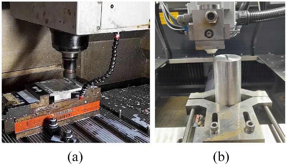
Manufacturing of the airfoils: (a) Machining of GOE404 and (b) Machining of MH42 using wire EDM.

Similar to the simulated profiles, algorithm 1 is used to extract the discrete profile for both GOE404 and MH42 profiles (i.e. Pe_GOE404, Pe_MH42). The parameter values, that is, Δm and θmin, are 10⁻⁴ and 178°, respectively. The number of points (i.e. n) was 10,000 in Pe_GOE404 and Pe_MH42. Later, the OBB and the dominant points for Pe_GOE404 and Pe_MH42 were computed using the OBB and algorithm 2 was implemented to get the OBB and dominant points of Pe_GOE404 and Pe_MH42.

The machined components are measured using GE PheonixVtome-XS240 Computed Tomography (CT) scanner (Figure 9(a)). The micro head of the CT-scanner is used for scanning purposes. The volumetric data acquisition and reconstruction were accomplished using the Pheonix dataosx software. Supplemental Table 8 shows the parameters considered during the measurement process.

Figure 9.

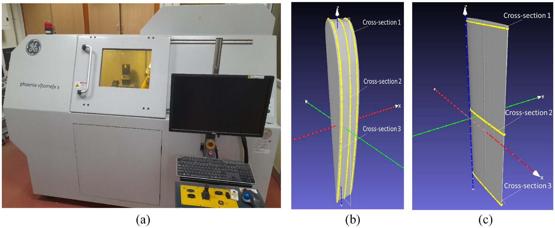
Measurement of airfoil profiles using a non-contact (CT) scanner: (a) GE CT-scanner used for measurement purpose, (b) STL model of GOE404 and (c) STL model of MH42.

VG studio 2.2 software was later used to process the CT scanner’s voxel data and STL model extraction. The STL models (both GOE404 and MH42) were sliced at three cross-sections using Meshlab software⁴⁸ (Figure 9(b) and (c)). The points along the sliced sections were considered as the measured point-set (Mc), and the proposed methodology is implemented for these measured point-sets.

The measured point-sets (Mc) of both GOE404 and MH42 are coarsely registered with Pe_GOE404 and Pe_MH42. Figure 10(a) shows the implementation of algorithm 3 for cross-section 2 of GOE404, and Figure 10(b) illustrate the same for MH42. Table 3(a) and (b) show the implementation results of algorithm 3 for both GOE404 and MH42 profiles.

Table 3.

Implementation results of stage B of the methodology for practically measured profiles θmin = 179°, $Δ$ m = 10⁻⁴.

Cross-section no.	No of points in Mc (m)	Coarse registration and fine-tuning (Mean. Sq. distance) (mm²)		Fine registration and profile error estimation			Absolute deviation (µm)		Gain in accuracy (%)
Cross-section no.	No of points in Mc (m)	Before	After	$e_{P_\max_PI}$ (mm)	$e_{P_\max_PCP}$ (mm)	$e_{P_\max_VEAW}$ (mm)	$d_{ab s_{PCP}}$	$d_{ab s_{VEAW}}$	Gain in accuracy (%)
(a) GOE 404 (n = 10,000)
1	1120	373.0785	0.0524	0.41739	0.41765	0.41742	0.2621	0.0250	90.46
2	1156	387.4003	0.0293	0.43282	0.43298	0.43284	0.1554	0.0174	88.81
3	1146	375.9898	0.0310	0.49106	0.49100	0.49110	0.0568	0.0398	29.93
(b). MH42 (n = 10,000)
1	1525	39.0275	0.0021	0.09105	0.09110	0.09104	0.0515	0.0080	84.47
2	1553	39.3178	0.0012	0.10066	0.10070	0.10066	0.0409	0.0018	95.60
3	1572	39.8327	0.0015	0.10397	0.10379	0.10397	0.1784	0.0045	97.48

Figure 10.

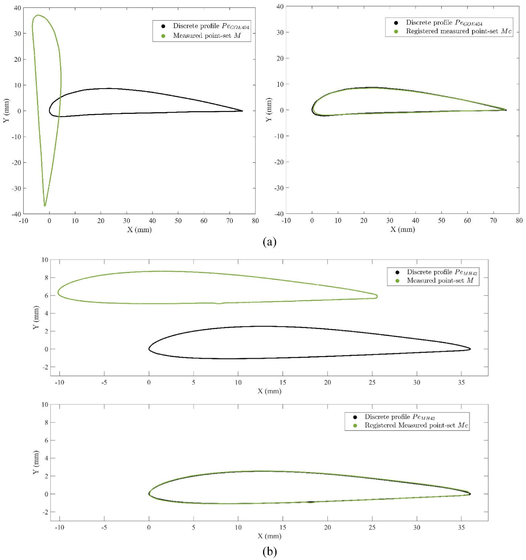
Implementation of Coarse registration and fine-tuning algorithm for practically measured profiles (algorithm 3): (a) GOE 404 and (b) MH42 (Cross-section 2).

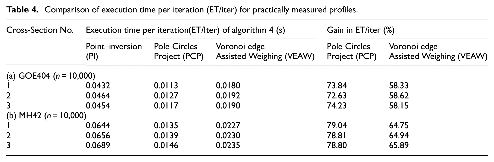
Similar to the simulated profiles (as mentioned in sec. 4.1.2), algorithm 4 is implemented for all the Mc’s. The corresponding profile error estimates (i.e. $e_{P_\max_PCP}$ and $e_{P_\max_VEAW}$ ) are validated using the point-inversion method (i.e. $e_{P_\max_PI}$ ). Table 3 shows the results of the implementation of algorithm 4. Supplemental Figure 11 depicts the convergence plots of algorithm 4 for GOE404 (cross-section 2) and MH42 (cross-section 2). The execution time per iteration (i.e. ET/iter of algorithm 4) is mentioned for each Mc (i.e. cross-sections) in Table 4.

Table 4.

Comparison of execution time per iteration (ET/iter) for practically measured profiles.

Cross-Section No.	Execution time per iteration(ET/Iter) of algorithm 4 (s)			Gain in ET/iter (%)
Cross-Section No.	Point–inversion (PI)	Pole Circles Project (PCP)	Voronoi edge Assisted Weighing (VEAW)	Pole Circles Project (PCP)	Voronoi edge Assisted Weighing (VEAW)
(a) GOE404 (n = 10,000)
1	0.0432	0.0113	0.0180	73.84	58.33
2	0.0464	0.0127	0.0192	72.63	58.62
3	0.0454	0.0117	0.0190	74.23	58.15
(b) MH42 (n = 10,000)
1	0.0644	0.0135	0.0227	79.04	64.75
2	0.0656	0.0139	0.0230	78.81	64.94
3	0.0689	0.0146	0.0235	78.80	65.89

Discussion

From Figures 6 and 10, it is observed that for both simulated and practically measured profiles, the Coarse registration and fine-tuning algorithm (algorithm 3) registers M with Pe within two steps. In Tables 1 and 3, it is observed that in all Mc’s, Mean Square Distance (MSD) significantly reduces upon implementing algorithm 3. In the case of the fine registration and profile error estimate algorithm (algorithm 4), as depicted in Supplemental Figures 8 and 11, the values of $e_{P_\max_PCP}$ and $e_{P_\max_VEAW}$ are closer to $e_{P_\max_PI}$ .

In Supplemental Figures 8(a) and 11(a), the values of $e_{P_\max}$ (for Mc corresponding to free-form profile 1 and cross-section 2 of GOE404) is initially not converging. This is attributed to the inherent limitation of the ICP method used in algorithm 4. However, after a few iterations, the values reducing. The linear convergence of the ICP method is evident in Supplemental Figures 8(b) and 11(b) after certain iterations.

Regarding the accuracy of PCP and VEAW techniques, d_abs′ values are considered the evaluation parameter. As observed in Tables 1 and 3, in all the cases, the d_abs are less than 1 µm (profile error in the scale of mm). Among $d_{ab s_{PCP}}$ and $d_{ab s_{VEAW}}$ , the values of $d_{ab s_{VEAW}}$ are relatively lower, thus indicating that the profile error estimates of the VEAW method are closer to that of the point-inversion method. Supplementary Figs.8 and 11 also depict the same. Even though PCP and VEAW method’s approximation is of order 2, the VEAW is a weighed method that estimates the Corres_pt_Mc and eventually the profile error more accurately. Upon comparing the respective d_abs values, a minimum of 29.93% (GOE404, cross-section 3) and a maximum of 98% (Profile 2) gain in accuracy is observed in the case of the VEAW method. In terms of execution time per iteration (ET/iter) (Tables 2 and 4), upon comparison to the point-inversion method, a maximum gain of 79.04% (PCP method, MH42, cross-section 1) and a minimum gain of 55.96% (VEAW method, profile 3, Table 3). However, in the former case, the difference between PCP and VEAW in terms of ET/iter is 6.7 ms, and in terms of accuracy, VEAW is 90.46% more accurate than PCP. Hence, VEAW is relatively more preferred than the PCP method.

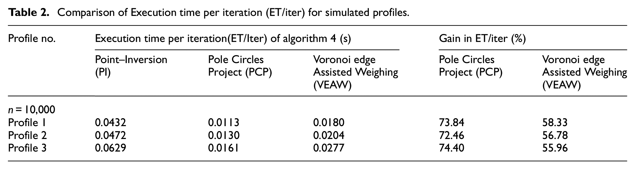
As observed in Tables 2 and 4, in all the cases, the ET/iter of the VEAW method is relatively higher. This is due to the excess time incurred for finding out the second nearest neighbour for each Mc_i $\in Mc$ and calculating the angular weights $α_{1}$ and $α_{2}$ (as explained in sec. 2.3). Each ET/iter (as mentioned in Table 2 and 4) is the average of 10 repetitive implementations executed for each cross-section. It was also ensured that the implementations for each cross-section were carried out afresh and independently. Overall, it is observed upon validation that both PCP and VEAW estimate the profile errors with accuracy in the order of a few micrometres, with the VEAW method having a minimum time gain of around 56%. However, as mentioned before, all the Pe’s contained only 10,000 points during the entire implementation. Higher accuracies can be attained by increasing the value of θmin, which eventually increases n’s value. However, this increases the ET/iter and thus the overall execution time of the fine registration and profile error estimation algorithm (algorithm 4).

Conclusion

A framework consisting of two stages is proposed for profile error estimation of 2D free-form profiles measured using either a CMM (operated in continuous scanning mode) or a non-contact scanner. Coarse registration is executed using the discretized profile (Pe) extracted using algorithm 1 (based on the concept of poles and pole angles). Two profile error estimation techniques (i.e. PCP and VEAW) were proposed and combined with the ICP based fine registration (algorithm 4). Implementations were executed for simulated as well as practically measured profiles. In practical implementations, the measured point-sets (M) were extracted from the CT scan data of two machined airfoil profiles (i.e. GOE404 and MH42). The summary of the implementations are as follows:

The OBB and dominant-points based coarse registration and fine-tuning algorithm align the measured point-sets within a few steps.

The results of validation (using the point-inversion method) of PCP and VEAW techniques illustrate that the VEAW technique is more accurate.

The proposed framework is at least 2.3x times (56%) faster than the point-inversion method.

Since the effective time-complexity is O(lm log n), this method can be considered a fast and accurate alternative to the point-inversion method. It can be used in the in-situ inspection of machined profiles accomplished using touch probes or vision-based systems associated with modern CNC machines. The future scope is to extend the method for 3D surfaces, partial scans of measured data and free-form objects represented as point-clouds and unstructured meshes. Moreover, the accuracy of the profile error estimation can be improved (with a relatively lower density of discretized profile) through new interpolation techniques that use the structure of the Voronoi diagram.

Supplemental Material

sj-docx-1-pib-10.1177_09544054221138173 – Supplemental material for A Voronoi diagram based framework for fast and accurate evaluation of 2D free-form profile errors

Supplemental material, sj-docx-1-pib-10.1177_09544054221138173 for A Voronoi diagram based framework for fast and accurate evaluation of 2D free-form profile errors by Hari Ganesh S and GL Samuel in Proceedings of the Institution of Mechanical Engineers, Part B: Journal of Engineering Manufacture

Footnotes

Appendix

Acknowledgements

The authors thank the people of the Center for Nondestructive Evaluation (CNDE) for the provision of the CT scanner.

Declaration of conflicting interests

The author(s) declared no potential conflicts of interest with respect to the research, authorship, and/or publication of this article.

Funding

The author(s) received no financial support for the research, authorship, and/or publication of this article.

ORCID iD

GL Samuel

Supplemental material

Supplemental material for this article is available online.

References

Savio

De Chiffre

Schmitt

Metrology of freeform shaped parts. CIRP Ann Manuf Technol 2007; 56(2): 810–835.

Ding

Yang

DCH

Han

Boundary-conformed machining of turbine blades. Proc IMechE, Part B: J Engineering Manufacture 2005; 219: 255–263.

Liu

Jia

, et al. Interpolation using non-uniform rational B-spline for the smooth milling of ruled-surface impeller blades. Proc IMechE, Part B: J Engineering Manufacture 2015; 229: 1118–1130.

Dong

Wang

A study of interferential tool position correcting algorithms in 3D impeller variable-axis rough plunge milling. Proc IMechE, Part B: J Engineering Manufacture. Epub ahead of print 10 May 2022. DOI: 10.1177/09544054221098609

Mali

Gupta

Ramkumar

A comprehensive review of free-form surface milling– advances over a decade. J Manuf Process 2021; 62: 132–167.

Mahboubkhah

Aliakbari

Burvill

An investigation on measurement accuracy of digitizing methods in turbine blade reverse engineering. Proc IMechE, Part B: J Engineering Manufacture 2018; 232: 1653–1671.

Bureau of Indian Standards. Geometrical tolerancing-tolerances of form, orientation, location and run-out. BIS, New Delhi, 2015.

Mian

Al-Ahmari

AM.

Application of the sampling strategies in the inspection process. Proc IMechE, Part B: J Engineering Manufacture 2017; 231: 565–575.

Rajamohan

Shunmugam

MS.

Strategies for measurement of sculptured surfaces using coordinate measuring machines in continuous scanning mode. Int J Mechatron Manuf Syst 2013; 6: 335–350.

10.

Zhou

Zhang

Tang

Sweep scan path planning for efficient freeform surface inspection on five-axis CMM. Comput Aided Des 2016; 77: 1–17.

11.

Zhang

Zhou

Tang

Sweep scan path planning for five-axis inspection of free-form surfaces. Robot Comput Integr Manuf 2018; 49: 335–348.

12.

Sang

Yan

Yao

, et al. A new scanning lines distribution strategy for the form error evaluation of freeform surface on CMM. Meas J Int Meas Confed 2021; 181: 109578.

13.

Free-form surface inspection techniques state of the art review. Comput Aided Des 2004; 36: 1395–1417.

14.

Ravishankar

Dutt

HNV

Gurumoorthy

AIWIN—a fast and jigless inspection technique for machined parts. Int J Adv Manuf Technol 2012; 62: 231–240.

15.

Mehrad

Xue

Robust localization to align measured points on the manufactured surface with design surface for freeform surface inspection. Comput Aided Des 2014; 53: 90–103.

16.

Jiang

Han

, et al. A workpiece registration and localization adjustment method with contact inspection under multi-tolerance conditions. Proc IMechE, Part B: J Engineering Manufacture 2019; 233: 1653–1662.

17.

Díez

Roure

Lladó

, et al. A qualitative review on 3D coarse registration methods. ACM Comput Surv 2015; 47: 1–36.

18.

Ghorbani

Khameneifar

Accurate Registration of point clouds of damaged aeroengine blades. J Manuf Sci Eng 2021; 143: 1–10.

19.

Besl

McKay

ND.

A method for registration of 3-D shapes. IEEE Trans Pattern Anal Mach Intell 1992; 14: 239–256.

20.

Brujic

Ristic

Monte Carlo simulation and analysis of free-form surface registration. Proc IMechE, Part B: J Engineering Manufacture 1997; 211: 605–617.

21.

Ravishankar

Dutt

HNV

Gurumoorthy

Automated inspection of aircraft parts using a modified ICP algorithm. Int J Adv Manuf Technol 2010; 46: 227–236.

22.

Yin

Huang

, et al. Three-dimensional point-based shape registration algorithm based on adaptive distance function. IET Comput Vis 2011; 5: 68–76.

23.

Xie

Yin

, et al. Variance-minimization iterative matching method for free-form Surfaces—Part I: Theory and Method. IEEE Trans Autom Sci Eng 2019; 16: 1181–1191.

24.

Xie

Yin

, et al. Variance-minimization iterative matching method for free-form Surfaces—Part II: Experiment and Analysis. IEEE Trans Autom Sci Eng 2019; 16: 1192–1204.

25.

Liu

Wang

, et al. WPMAVM: Weighted plus-and-minus allowance variance minimization algorithm for solving matching distortion. Robot Comput Integr Manuf 2022; 76: 102320.

26.

Zhu

Zhang

Chen

, et al. A methodology for measuring and evaluating geometric errors of aero-engine blades based on genetic algorithm. Proc IMechE, Part B: J Engineering Manufacture 2020; 234: 260–269.

27.

Rajamohan

Shunmugam

Samuel

GL.

Effect of probe size and measurement strategies on assessment of freeform profile deviations using coordinate measuring machine. Measurement 2011; 44: 832–841.

28.

Piegl

Tiller

Monographs in visual communication. Berlin, Heidelberg: Springer, 1997.

29.

Zhang

, et al. Fast evaluation of minimum zone form errors of freeform NURBS surfaces. Procedia CIRP 2015; 27: 23–28.

30.

Sakkalis

Orthogonal projection of points in CAD/CAM applications: an overview. J Comput Des Eng 2014; 1: 116–127.

31.

Pan

, et al. A geometric strategy algorithm for orthogonal projection onto a parametric surface. J Comput Sci Technol 2019; 34: 1279–1293.

32.

Lang

Song

, et al. Profile error evaluation of free-form surface using sequential quadratic programming algorithm. Precis Eng 2017; 47: 344–352.

33.

Sang

Wang

, et al. A profile error evaluation method for freeform surface measured by sweep scanning on CMM. Precis Eng 2019; 56: 280–292.

34.

Liu

Calculation of profile error for complex surface. Measurement 2014; 48: 183–186.

35.

Biradar

Pande

SS.

Efficient algorithms for automated inspection of Freeform surfaces. Procedia Manuf 2015; 1: 35–46.

36.

Dey

TK.

Curve and surface reconstruction algorithms with mathematical analysis. Cambridge: Cambridge University Press, 2007.

37.

Samuel

Shunmugam

MS.

Evaluation of circularity from coordinate and form data using computational geometric techniques. Precis Eng 2000; 24: 251–263.

38.

OuYang

Feng

H-Y

Jahangir

, et al. Robust initial matching of free-form objects represented by point clouds. J Manuf Sci Eng 2012; 134: 021008.

39.

Amenta

Bern

Surface Reconstruction by Voronoi filtering. Discrete Comput Geom 1999; 22: 481–504.

40.

Amenta

Kolluri

. Accurate and efficient unions of balls. In: Proceedings of the sixteenth annual symposium on computational geometry, 2000, pp.119–128. New York: ACM.

41.

Amenta

Choi

Kolluri

RK.

The power crust, unions of balls, and the medial axis transform. Comput Geom Theory Appl 2001; 19: 127–153.

42.

Hari Ganesh

Samuel

. A 3D Voronoi diagram based form error estimation method for fast and accurate inspection of free-form surfaces. Measurement 2022; 189: 110476.

43.

Chung

Yun

Lee

SU.

Registration of multiple-range views using the reverse-calibration technique. Pattern Recognit 1998; 31: 457–464.

44.

Liu

Wong

Zhang

, et al. Adaptive fairing of digitized point data with discrete curvature. Comput Aided Des 2002; 34: 309–320.

45.

De Berg

Cheong

Van Kreveld

, et al. Computational geometry: Algorithms and applications. 3rd ed. Berlin Heidelberg: Springer-Verlag, 2008.

46.

UIUC Airfoil Coordinates Database. https://m-selig.ae.illinois.edu/ads/coord_database.html, UIUC Applied Aerodynamics Group, Department of Aerospace Engineering, University of Illinois Urbana-Champaign. (accessed 8 December 2021).

47.

Airfoil Dat to NURBS, Flusur, https://www.flusur.com/dat2nurbs/ (accessed 8 December 2021).

48.

Cignoni

Callieri

Corsini

, et al. MeshLab: An open-source mesh processing tool. In: 6th Eurographics Italian chapter conference 2008 - proceedings2008, pp.129–136.

Supplementary Material

Please find the following supplemental material available below.

For Open Access articles published under a Creative Commons License, all supplemental material carries the same license as the article it is associated with.

For non-Open Access articles published, all supplemental material carries a non-exclusive license, and permission requests for re-use of supplemental material or any part of supplemental material shall be sent directly to the copyright owner as specified in the copyright notice associated with the article.

0.00 MB

1.45 MB