
Abstract
The cement specific surface area is an important indicator of cement quality. The accurate prediction of the cement specific surface area aims to guide operators to control the cement grinding process to improve product quality while reducing system energy consumption. However, due to the complexity of the cement grinding process, the process variables have coupling, time-varying delay, nonlinear characteristics, and different sampling frequency. Herein, we proposed the specific surface area prediction model, which combined dual-frequency principal component analysis and extreme gradient boosting (DF-PCA-XGB). In order to solve the problem of difficulty in modeling due to different sampling intervals of related data, this paper analyzes the low-frequency sampling data and high-frequency sampling data under multiple working conditions, and establishes prediction models respectively. Aiming at the data redundancy problem of high-frequency and low-frequency variable data in the introduced time window, a method based on the combination of principal component analysis (PCA) and extreme gradient boosting (XGB) cross-validation is proposed to reduce data redundancy while retaining most of the characteristics of the data. The final specific surface area prediction results were obtained by weighting the high-frequency data model and the low-frequency data model. The simulation results showed that the prediction method in this paper can improve the prediction accuracy of the specific surface area of the finished cement product under multiple working conditions with high stability and has promising application in the cement manufacturing process.
Keywords
Introduction
The cement specific surface area is the total surface area of the cement powder per unit mass, 1 which is an important indicator for evaluating cement quality. The problems in the cement grinding process, including data sampling frequency differences and data redundancy, can affect the service life of the concrete. 2 The accurate prediction of the specific surface area of the finished cement product provides a basis for the optimization control of the cement mill system and the improvement of the quality of the finished cement product. 3 Therefore, the study of prediction of cement specific surface area is of great importance for high quality and intelligent manufacturing of cement.
The cement mill grinding process is a complicated process. When entering the cement mill system, the cement undergoes two processes, including preliminary grinding by the coarse grinding system and further grinding by the fine grinding system. Before entering the cement finished product warehouse, the specific surface area of the finished cement is measured in the laboratory. 4 The cement mill runs under multiple working conditions, and different process variables have various sampling intervals, distinct frequencies, and data redundancy. Simply putting data with different time intervals into the time window 5 may cause the data features to be incorrectly extracted and reduce the accuracy of the prediction model.
The above-mentioned problems have posed great difficulties to build an accurate specific surface area prediction model. In Wang, 6 the unitary linear regression method is used to quickly predict the specific surface area of cement with 45 μm fineness, and in detail, the 45 μm sieve residue of the cement was detected by the negative pressure sieve analysis method and the determination of the cement specific surface area. Then, the obtained data is subjected to regression analysis to establish a linear equation of 45 μm cement fineness and specific surface area, thus realizing the prediction of specific surface area. In Wu et al., 7 for the modeling of the combined grinding system with cement particle size, a regression analysis algorithm was used to establish a multiple input single output particle size model and a least square support vector machine (LSSVM) was used to predict the cement particle size. In this paper, we proposed a prediction model of cement specific surface area based on PCA and XGB. The main advantages of this model are summarized as follows.
(1) To reduce the redundancy of time series data, PCA are used to select the principal components of high and low frequency variable data respectively.
(2) In order to eliminate the interference caused by different sampling time intervals to the prediction model, the high-frequency variable data prediction model and the low-frequency variable data prediction model after the main component selection are established respectively based on XGB.
(3) The final prediction result obtained from combining the high-frequency and the low-frequency variable prediction model can improve the prediction accuracy.
Related work
As mentioned in the first chapter, in the grinding process of the cement mill system, the sampling period of each variable is different, and the data is characterized by a large amount of redundancy, nonlinearity, and coupling between variables.
In order to solve the problem of difficult prediction caused by the different sampling period of each variable, Zhongda et al. 8 used control loop dynamic weights, network utilization, and data transmission time to determine the variable sampling period of each control loop. This method realizes the control of the variable sampling period, but there is no good method to solve the problem of using the data of different sampling periods to predict.
Aiming at the problem of a large amount of data redundancy, Wang et al. 9 used feature selection techniques to find the most effective features and reduce redundant features. Computational cost is reduced by reformulating within class scatter matrix through minimum Redundancy Maximum Relevance (mRMR) algorithm while preserving discriminant information. 10
In order to solve the problems such as non-linearity and coupling, traditional machine learning algorithms are well used in fingerprint recognition,11,12 fault diagnosis,13,14 energy consumption prediction,15,16 and other fields. In recent years, the extreme gradient boosting algorithm has been applied to fault detection,17,18 classification problems,19,20 model prediction,21,22 and other fields due to its excellent performance. In Zamani Joharestani et al., 23 23 features such as ground-measured PM2.5 and geographic data are used for modeling through XGB to achieve accurate PM2.5 prediction. In Li et al., 24 gene expression values are predicted by a prediction algorithm based on XGB. XGB uses the first derivative and the second derivative at the same time, so the loss is smaller.
The cement production process has the characteristics of multivariable and time-varying time delay. 25 In view of the characteristics of the cement production process data, some current methods adopt the method of constructing a time window, 26 sorting multiple variables in a time series, and constructing the model input layer. 15 However, the cement mill system runs under multiple working conditions, the sampling time interval of different process variables is different, and there is a large amount of data redundancy in the time window data. 27
Based on the above analysis, this paper establishes a specific surface area prediction model based on PCA and XGB.
Cement mill process analysis
The operating status of the cement mill system directly affects the cement specific surface area. 28 The cement mill system is shown in Figure 1. A variety of raw materials enter the feeding bin according to a certain ratio, and enter the roller press for preliminary grinding under the control of the roller press baffle. 29 The ground material enters the powder separator under the action of the feed elevator, and the material is separated in the powder separator. In the middle layer, the unqualified materials are returned to the roller press for grinding, and this part forms the rough grinding system. 30 When working normally, the host current, the current drawn by the feed hopper, and the abrasive hopper are relatively stable, and the feed and output of the mill are balanced. The materials are fully ground to obtain a qualified surface area product. When the full grinding operation occurs, both the main engine current and the current drawn from the grinding bucket are relatively large. The inability of the material to be completely ground causes the specific surface area of the cement to be too large.
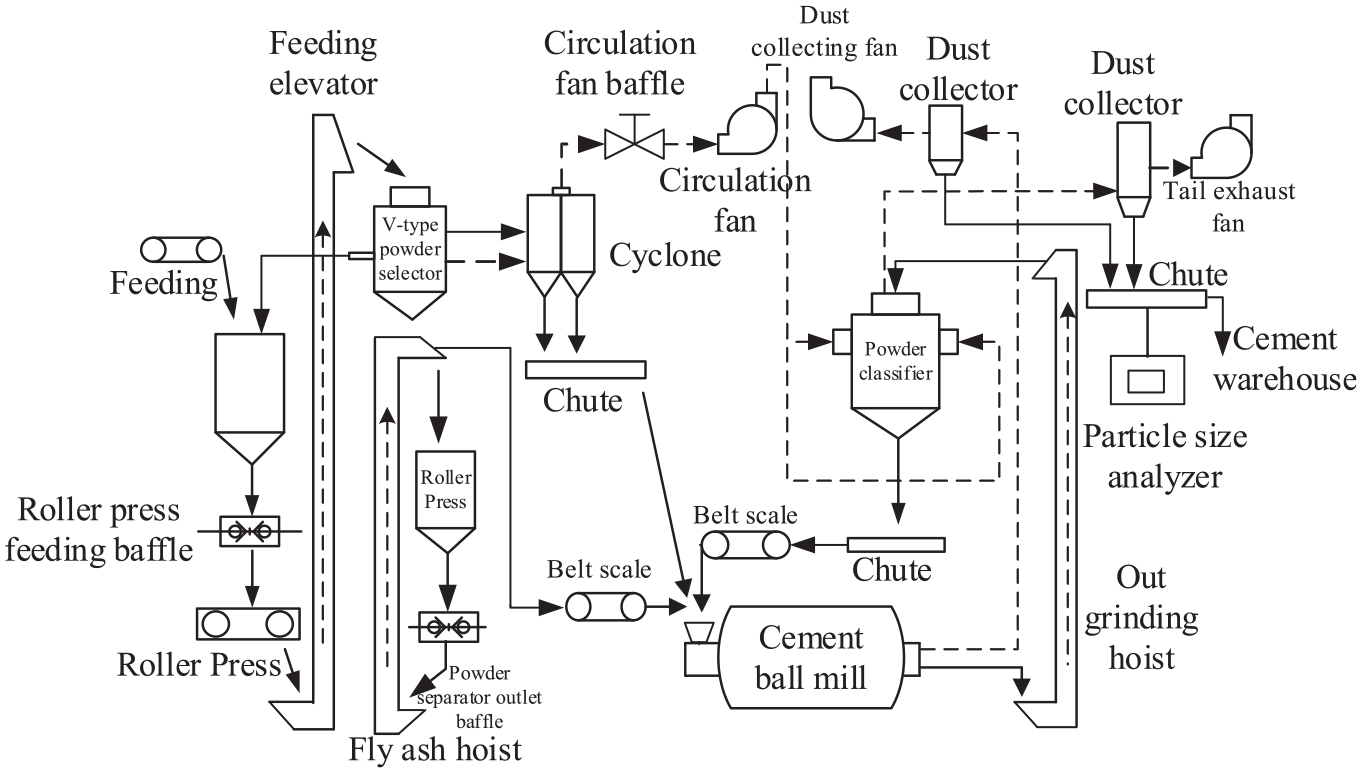
Equipment composition and production diagram of cement mill system.
Through the analysis of the above cement mill technology, nine key process variables that affect the specific surface area of cement are obtained. The variables with small sampling intervals are defined as high-frequency variables: host current (
The prediction model based onDF-PCA-XGB
This section builds a prediction model based on the key variables with different sampling intervals obtained from the cement mill process analysis in the previous section. The PCA and XGB are used to select the principal components of the data at different sampling intervals in the time window, which reduces data redundancy while retaining most important features.
The structure of the DF-PCA-XGB
The prediction model framework of DF-PCA-XGB is shown in Figure 2. First, the key variable data in the cement industry database is extracted. Then the data is divided into high-frequency variable data and low-frequency variable data. The PCA and XGB are combined to select the principal components of the data at different sampling intervals. Finally, we combined the XGB algorithm to build a specific surface area prediction model to complete the specific surface area prediction.
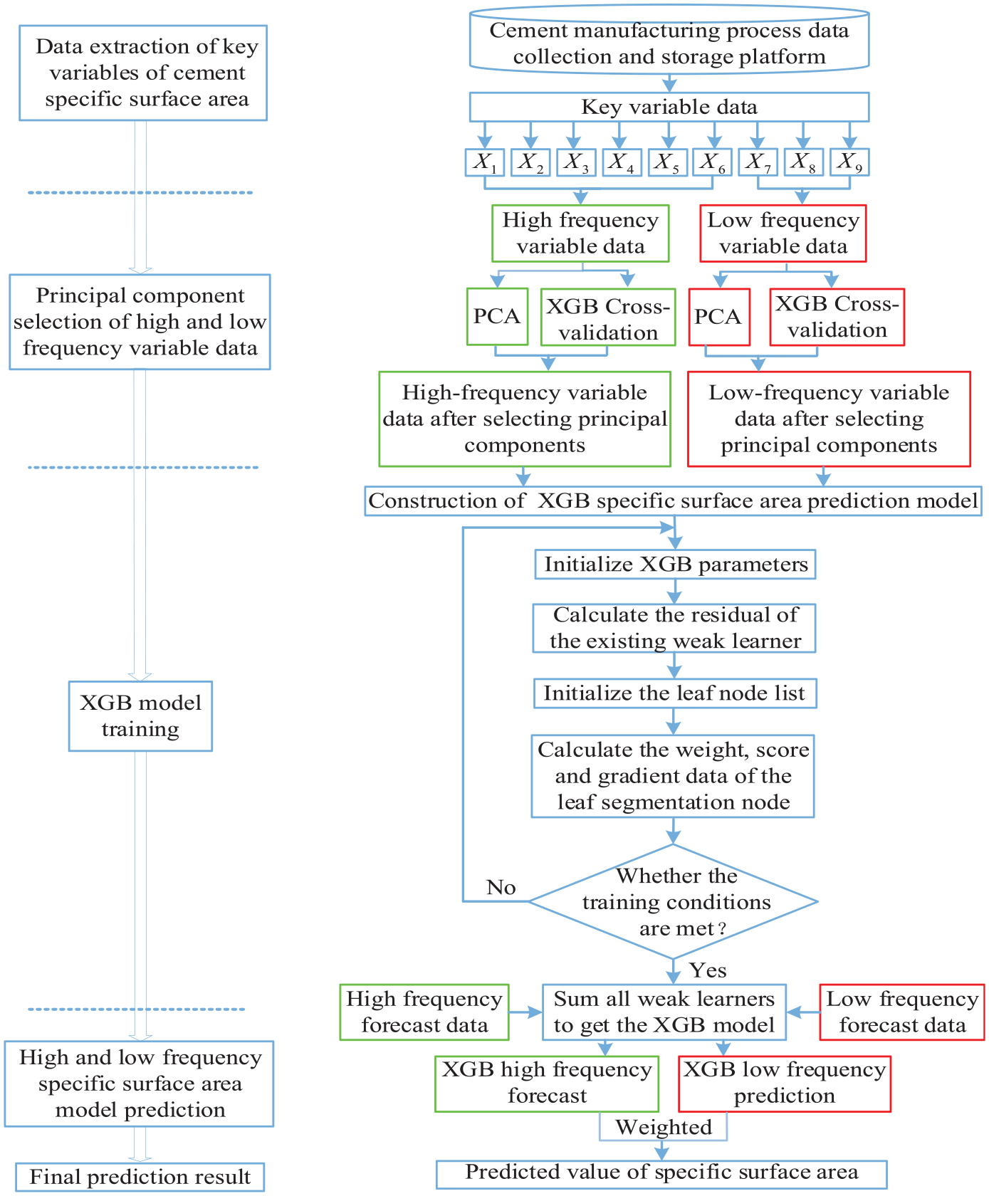
Prediction model framework based on DF-PCA -XGB.
Data analysis based on PCA
Aiming at the problem of different data redundancy in different sampling time intervals when constructing the time window, this section conducts principal component analysis on variables of different sampling time intervals. We use a combination of PCA and XGB cross-validation to select the principal components of the data at different sampling intervals.
The principal component analysis steps of specific surface area production data based on PCA are as follows 31 :
(1) The specific surface area production data is decentralized, and each specific surface area feature is subtracted from the mean value of the feature, so that
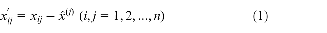
Where
(2) Perform singular value decomposition on the decentralized specific surface area production data

(3) Then obtain the eigenvalue

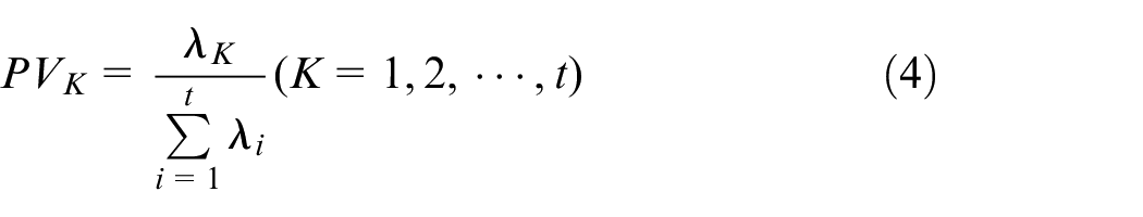
(4) Sort the eigenvalues of the high-frequency variable data and the low-frequency variable data in order from small to large, and calculate the principal component contribution rate
(5) Obtain the rate of change of contribution rate
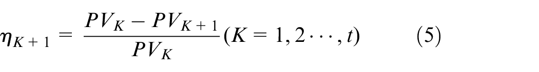
Where
(6) Combine XGB to perform
The prediction model of specific surface area based on XGB
Based on the PCA comparison surface area production data for the selection of principal components, this section uses the specific surface area production data after the principal components are selected to construct the input and output layers of the XGB model. The flow chart of specific surface area prediction algorithm based on XGB is shown in Figure 3. XGB is a tree ensemble model. 32
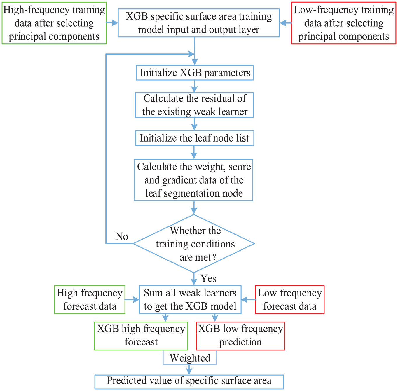
Flow chart of specific surface area prediction algorithm based on XGB.
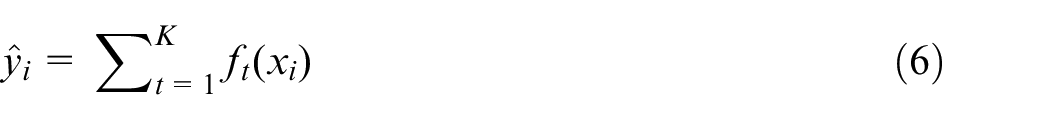
The derivation process of the XGB-based specific surface area prediction algorithm is as follows:
The specific surface area training data is assumed to be a data set
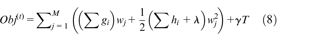
The prediction accuracy of the XGB model is determined by the bias and variance. The loss function of the model reflects the deviation of the model. And the variance of the model is controlled by the regularization term. The loss function and the regularization term together constitute the objective function of the XGB model:
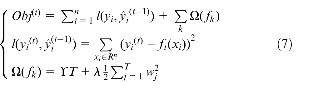
Where
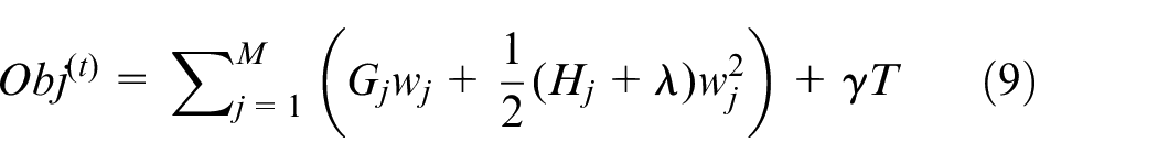
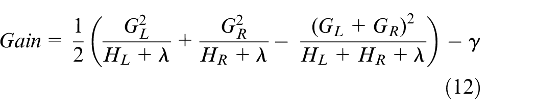
In order to improve the convergence speed of the model, XGB performs a second-order Taylor expansion on the loss function in the tree building process, introduces the second-order derivative information, groups the objective function according to leaf nodes, and defines
Where
In the above formula, the leaf node score
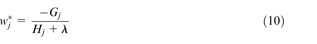
Substitute the optimal value
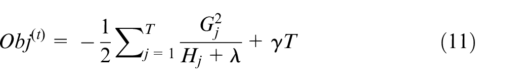
Where
If the maximum gain is 0, the current decision tree is established, and the weak learner
Experimental results and analysis
Data redundancy and difference experiment
Extract the specific surface area production data from the energy management database of Tangshan Sanyou Jidong Cement Enterprise, and divide it into high-frequency variable data and low-frequency variable data according to the sampling time interval.
In order to verify that the data redundancy of different sampling time intervals is different, this section conducts principal component analysis on high and low frequency variable data based on PCA, and uses the cumulative variance contribution rate as the criterion for data feature loss. The higher the cumulative variance contribution rate, the less the loss of data features. Figure 4(a) and (b) are graphs of the cumulative variance contribution rate of high and low frequency variable data respectively.
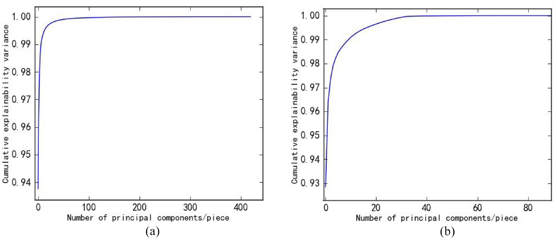
(a) Cumulative variance contribution curve of high-frequency variable data and (b) cumulative variance contribution curve of low-frequency variable data.
It can be seen from Figure 4(a) and (b) that the slope of the cumulative variance contribution rate curve of the high and low frequency variable data decreases as the number of principal components increases. Among them, when the number of principal components of high-frequency variable data is greater than 100, the cumulative variance hardly increases; when the number of principal components of low-frequency variable data is greater than 40, the cumulative variance contribution rate increases extremely slowly.
In order to show the relationship between the number of principal components and the cumulative variance contribution rate more specifically, the contribution rate and cumulative contribution rate of the first 10 principal components of the high and low frequency variable data are taken. The data is shown in Table 1.
Top 10 principal components contribution rates and cumulative contribution rates for high and low frequency data.
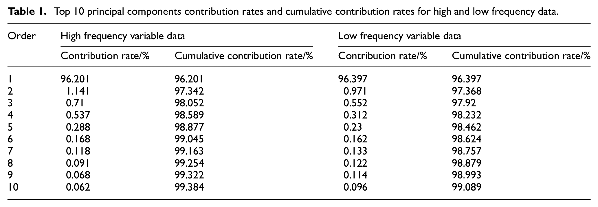
It can be seen from Table 1 that the contribution rates of the first-order principal components in the high and low-frequency variable data are 96.201% and 96.397%, respectively, indicating that the first-order principal components contain most of the characteristics of the specific surface area production data. Since then, the contribution rate of the principal components of each order gradually decreases, and the rate of decline slows down with the increase of the order, until the contribution rate of the principal component of the high and low frequency variable data of the 10th stage is less than 0.1%, and the cumulative variance contribution rate of the first 10 principal components reaches 99 % the above. Experiments have proved that there is a lot of redundant information in the specific surface area production data and the first 10-order principal components can represent most of the original data characteristics.
Determination of the number of principal components of data
Principal component selection is performed by calculating the principal component contribution rate and cumulative contribution rate for the high and low frequency variable data, and determining the principal component number interval
Figure 5(a) and (b) show the model learning curve when the high and low frequency variable data has different principal components. The number of principal components after the high frequency variable data is selected is 32, and the number of principal components after the low frequency variable data is selected is 46. Select the first 32-order principal components of the high-frequency variable data and the first 46-order principal components of the low-frequency variable data to construct the input and output layer of the prediction model.
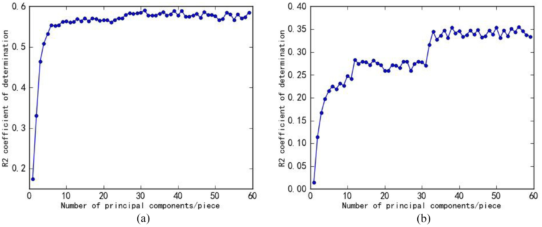
(a) Model learning curve after main components selection of high-frequency variable data and (b) model learning curve after main components selection of low-frequency variable data.
Further, the experimental exploration of joint prediction of high and low frequency variable data is carried out. By traversing the prediction results of the two prediction models, the weights of the high frequency prediction model and the R2 curve after the main component selection are obtained as shown in Figure 6.
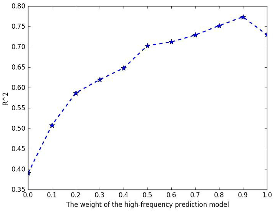
High-frequency prediction model weight and R2 curve.
The results in Figure 6 show that when the high-frequency prediction model weight is 0.9 and the low-frequency prediction model weight is 0.1, the prediction accuracy is the highest.
Specific surface area prediction based onDF-PCA -XGB
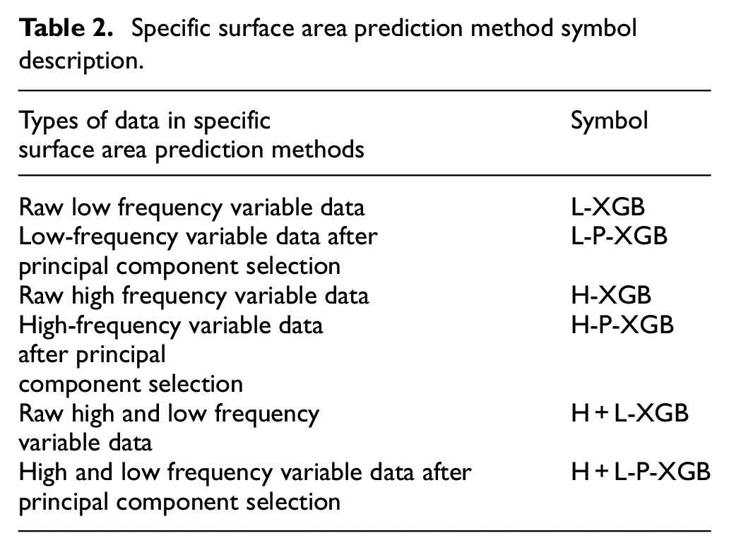
In order to reflect the effectiveness of the method proposed in this article, through the method in this paper, the data set after the principal component selection is obtained, and compared with the original data set. For the convenience of explanation, the specific surface area prediction method is replaced by the symbols in Table 2.
Specific surface area prediction method symbol description.
This paper uses root mean square error (RMSE), average absolute error (MAE), and R2 coefficient of determination as evaluation indicators. 33 Experiment with the above six methods to draw a histogram of each indicator as shown in Figure 7.
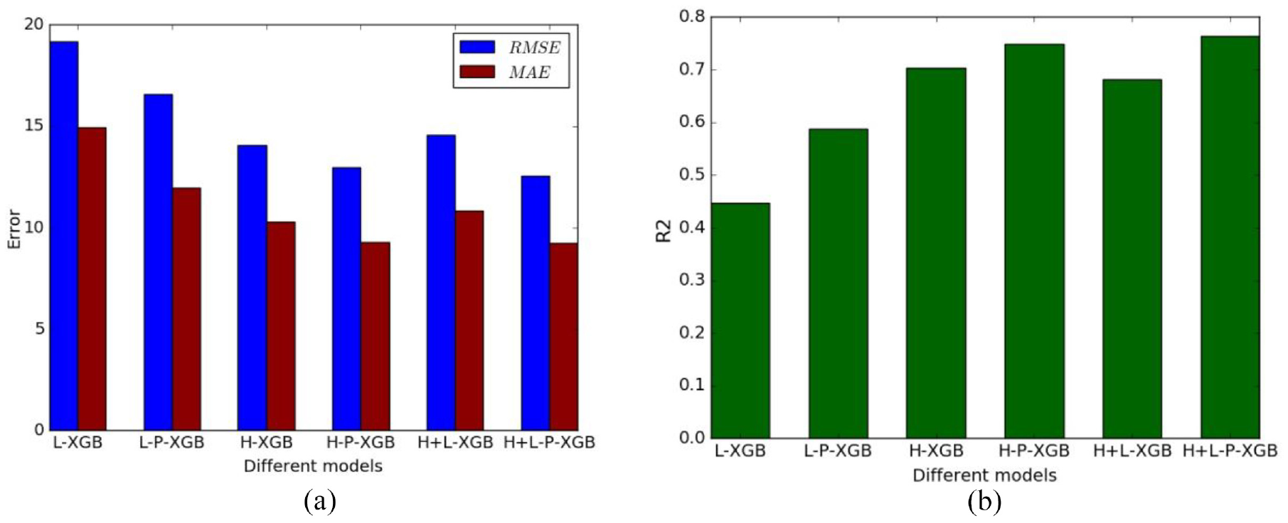
Predictor histogram: (a) error histogram and (b) R2 histogram.
As shown in Figure 7(a) and (b), the high specific surface area and low frequency variable data after the main component selection have lower prediction errors than the corresponding original data, and the R2 determination coefficient is higher. The results show that the combined prediction model of high and low frequency variable data obtained by the method of this paper has the best effect and the highest accuracy after the main components are selected, which verifies the effectiveness of the method proposed in this paper.
Use different types of specific surface area production data to build XGB specific surface area prediction models, and conduct model training and prediction. Figures 8 and 9 are the prediction comparison diagrams of the high-frequency and low-frequency raw data and the data after the main component selection.
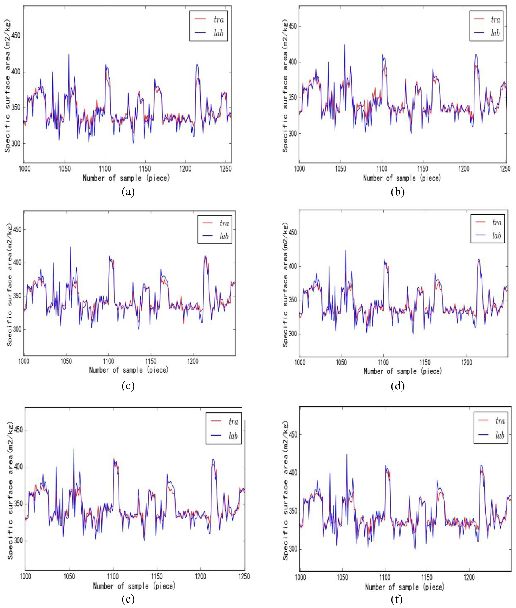
Specific surface area training chart of different data: (a) L-XGB, (b) L-P-XGB, (c) H-XGB, (d) H-P-XGB, (e) H+L-XGB, and (f) H+L-P-XGB.
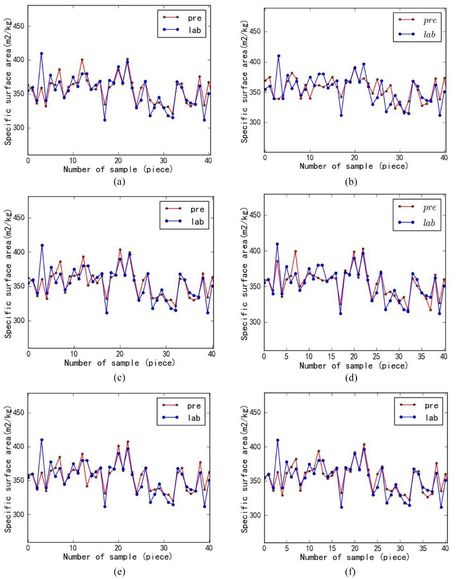
Specific surface area prediction chart of different data: (a) L-XGB, (b) L-P-XGB, (c) H-XGB, (d) H-P-XGB, (e) H+L-XGB, and (f) H+L-P-XGB.
Among the training curves and prediction curves shown in Figures 8 and 9, H+L-P-XGB has the best fitting effect, and each evaluation index is also the best. Experimental results show that extracting high and low frequency specific surface area production data separately for specific surface area prediction can eliminate the interference caused by different sampling intervals on the prediction model. In the cement production process, when the production indicators are determined, each process is executed in an orderly manner, and there are a large number of similar working conditions, resulting in high production data redundancy. PCA and XGB cross-validation are combined to select the principal components of the high and low frequency variable data respectively, which can reduce the redundancy of the high frequency variable data and the low frequency variable data, and retain the characteristics of the high and low frequency variable data. Based on XGB, the high-frequency variable data prediction model and the low-frequency variable data prediction model after the principal component selection are established respectively. The two models are weighted to obtain the final prediction result, which can eliminate the interference caused by the different sampling time intervals on the prediction model, while retaining the characteristics of high and low frequency variable data are improved, and the prediction accuracy of the model is improved.
Conclusion
This paper establishes a prediction model for the cement specific surface area based on DF-PCA-XGB. The input data is divided into high-frequency data and low-frequency data, which avoids the problem of difficult modeling caused by different data frequencies. A method of combining PCA and XGB cross-validation to select principal components is proposed to reduce data redundancy while ensuring that the main characteristics of the data are not lost. According to the high and low frequency variable data selected by the principal components, the input and output layer of the prediction model is constructed, and the high and low frequency joint prediction model of specific surface area based on PCA and XGB is established. The final predicted value of specific surface area is obtained by weighting. The experimental results show that the variable data principal component analysis of the combined forecasting method proposed in this paper combined with XGB eliminates the influence of different sampling intervals on the establishment of the forecasting model and reduces the redundancy of time series data. The prediction accuracy is significantly improved to meet the industrial production standard. The accurate prediction of specific surface area is beneficial to guide the production scheduling of cement mill systems and improve the manufacturing quality of cement.
The application of DF-PCA-XGB model can not only provide reference for cement grinding quality, but also provide theoretical support for cement grinding process optimization and intelligent control.
Footnotes
Declaration of conflicting interests
The author(s) declared no potential conflicts of interest with respect to the research, authorship, and/or publication of this article.
Funding
The author(s) disclosed receipt of the following financial support for the research, authorship, and/or publication of this article: This work is supported by the National Natural Science Foundation of China (Grant No. 62073281), the Hebei Provincial Natural Science Foundation (Grant No. F2019203385), the Hebei Provincial Science and Technology Plan Project (Grant No. 19211602D), the Second Batch of Youth Top-notch Talent Support Program in Hebei Province (Grant No. 5040050).