Sage Journals: Discover world-class research

Abstract

Finned tube air heat-exchangers are built by joining the tubes to the fins by various techniques. A technique mostly used for large heat-exchangers consists of fitting the tubes into the holes of the fins by expanding the tubes using a mechanical process. The expansion is achieved by inserting an ogive of a larger diameter into the tube. The intimate contact of tubes and fins due to the press fitting ensures the proper thermal connection. This work tries to describe an experimental-numerical procedure useful to study and predict the mechanical process and the process parameters. The procedure, based on material properties obtained from tensile tests and the use of the inverse method to identify the material parameters, is based on bi-dimensional finite element (FE) models used to simulate the expansion process. The FE model is then used for process optimisation regarding such parameters as the ogive shape and ogive sizes, friction coefficient and speed of insertion of the ogive into the tube. Indeed, size and shape uncertainties strongly influence the process parameters and the process quality, as well as the heat-exchanger efficiency. The use of numerical models was proven highly effective in predicting and optimising the process by quickly analysing the influencing factors and optimising the production.

Keywords

Air heat-exchanger manufacturing tubes mechanical expansion process simulation plasticity FEM simulation

Introduction

In the type of air heat-exchangers made with fins, the tubes can be made of copper, nickel or other metal alloys. The fins have a regular pattern of holes in which tubes are fitted and assembled into packs. The optimal thermal connectivity between the tubes and the fins, which gives the maximum exchange of heat between the fluid (circulating in the tubes) and the air (passing over the fins), is obtained when the contact area between them is maximised, and this can be achieved either by using some intermediate highly conducting materials, that is some soldering metal, or by press fitting, when a radial homogeneous pressure is exchanged in the contact area. This press fitting assembly can be obtained by plastically expanding the tubes, and the expansion can be hydraulic or mechanical. As discussed by MacGregor et al.,¹ in the hydraulic expansion, a fluid is introduced in the tube and pressurised at a required level. As discussed by Avalle et al.,² in the mechanical expansion process, the external diameter of the tube is made larger than the diameter of the holes in the fins through the insertion of a tool. The diameter of the tool is larger than the internal diameter of the tube. The tool can be a sphere or an ogive, in any case with an axisymmetric section. Usually, the sphere is pushed through the tube by a fluid with a suitable pressure applied from one end of the tube itself. The ogive, instead, is pushed mechanically by a rod. In the hydraulic expansion process, the size and shape of the final connection depends on the stiffness of the parts, tubes and fins; local variations due to, for example, material variations or thickness variations are difficult to control and can give unpredictable results. On the contrary, the mechanical expansion process is strongly affected by interference, that is by the effective diameters of the parts; these geometrical parameters must be precisely controlled to avoid manufacturing uncertainties. In the mechanical expansion process, the method based on the insertion of the sphere is less controllable because the movement (speed) of the sphere depends on the resistance encountered during insertion. When using the ogive, pushed by a rod, the insertion speed is imposed; the system is simpler, but the ogives are more expensive due to their complex shape. In general, the mechanical expansion process is cheaper and more versatile. It is more interesting, especially for producing smaller heat-exchangers and small series or for individual production, where each single product is made on purpose and is unique. The hydraulic expansion method is more commonly used in petroleum production, while mechanical expansion is used in heat-exchanger production and energy absorption applications. The hydraulic expansion method was studied by Hwang and Altan³ in the case of a circular tube expanded to a rectangular cross-section. The hydroforming process of aluminium tubes was investigated by Abrantes et al.,⁴ whereas the expansion of stainless-steel tubes using the hydroforming process was studied by Gao and Strano,⁵ and this process optimised the pre-bending phase using numerical simulations. In the same field, a control algorithm in combination with FE models was developed by Ray and MacDonald⁶ to optimise the hydroforming process of the tubes.

Several works in the technical literature have dealt with the study of the mechanical expansion process of tubes for various applications with various materials and with different approaches: considering the energy absorption applications, a theoretical prediction supported by an experimental investigation was carried out by Tan et al.⁷ Theoretical analyses and models were also proposed by Wu et al.,⁸ Luo et al.⁹ and Liu and Qiu.¹⁰ The plastic energy absorption of the aluminium tubes when the expansion was performed with conical-cylindrical die was analysed by Yang et al.¹¹

The expansion of the tubes used in the petroleum industry was analytically investigated by Hwang and Chen¹² and by Pervez et al.^13,14 working with FE models¹³ and experimental tests.¹⁴ The aluminium and steel tubes expanded for this application were also investigated by Seibi et al.,¹⁵ who carried out an experimental study designed for the mechanical expansion of the tubes. The same author proposed^16,17 a mathematical model of the expanded tube.

Focussing on the production of fluid pipe circuits and heat-exchangers, the tube-to-tubesheet joints were discussed by Alves et al.,¹⁸ who presented a new deformation process, and by Bouzid and Zhu,¹⁹ who studied the effect of the residual contact pressure between the two parts. They also developed an analytical model where the effects of strain-hardening²⁰ and of reverse yielding²¹ were introduced and shown. The expansion of the tubes made of copper was analysed by Tang et al. in different works. In Tang et al.,²² they studied both from a numerical and an experimental viewpoint the deformation and contact between microgroove tube and aluminium fins. In Tang et al.,²³ they investigated the influence of the groove shape of the tubes on the quality of the forming (expansion) process. In Tang et al.,²⁴ they optimised the expansion process, developing a method based on numerical simulations and experimental tests. For example, they focussed on the shape of the fin collar to increase the contact surface between the tube and the fin. The contact area between the tube and the fin was also studied with numerical simulations by Kwon et al.,²⁵ whereas Kang et al.²⁶ developed three-dimensional groove tubes to increase further the efficiency of heat-exchangers.

As for other applications, in this field, numerical simulation by means of finite element models is a fundamental instrument to develop studies on the tube expansion process. Avalle et al.² designed an FE model, starting from experimental tests, to evaluate the effects of the process parameters. Scattina²⁷ used a three-dimensional FE model to study the effects of the tolerance errors of the tubes on the expansion process. Numerical models are also often used to develop analytical models on the subject, as proposed by Karrech and Seibi,²⁸ who developed a mathematical model to evaluate the stress state of the deformed part and the drawing force of the process, or by Alves et al.,²⁹ who conducted experimental tests on AA6060 aluminium alloy tubes, comparing the results with a numerical model and evidencing the importance of issues with modelling friction during the process. The same model was also used in Alves et al.³⁰ to study a related application, such as the hydroforming of carbon tubes. In Gouveia et al.,³¹ the formability of aluminium tubes and the effects of the process parameters using numerical simulations were investigated. The numerical models were also used to study the effects of several configurations (expansion method, alloy, pipe loading) on the mechanical properties of the steel subjected to tubular expansion, as proposed by Mack,³² or to investigate the effect of the process parameters, as proposed by Avalle et al.^2,33 and Han et al.,³⁴ who used the expansion force rate to define the amount of adhesion in the tube’s inner grooves.

In this overview, the aim of the present work is to describe the procedure of designing the tube-expansion process for finned air heat-exchangers, starting from material characterisation to obtain a numerical model of the expansion process. This FE model will describe the influence of the process parameters and will thus guide the selection and definition of the optimal process parameters, depending on the materials and characteristics of the tubes and fins.

Experimental characterisation: Material properties and driving force

Material properties

The mechanical properties of the tube materials were defined by performing a series of tensile tests. The experimental tests were carried out by means of an Instron 8801 testing machine. The setup of the tests was according to the standard ASTM E8M-16a. This standard deals with tube specimens. In this work, AISI 316 stainless steel tubes were studied. This material is mostly used to produce the type of heat-exchangers under consideration; therefore, an improvement in the analysis of the production process could satisfy industrial requirements. Other materials typically used to produce this type of heat-exchanger were studied by the authors in previous works: copper-nickel alloys by Avalle et al.² and titanium by Avalle and Scattina.³³ The tube samples for tensile tests had a length L of 208–210 mm and an external diameter D_e of 15.875 and 19.05 mm (non-expanded tube, see Table 1).

Table 1.

Test speed of the tensile tests for the examined stainless steel.

Thickness (mm)	External diameter
	D_e = 15.875 mm		D_e = 19.05 mm
t = 0.89	0.1	mm/s	–	mm/s
	5		–
t = 1	–	mm/s	0.1	mm/s
	–		5
t = 1.25	0.1	mm/s	–	mm/s
	5
t = 1.5	–	mm/s	0.1	mm/s
			5
t = 1.65	0.1	mm/s	0.1	mm/s
	5		5
	100		100

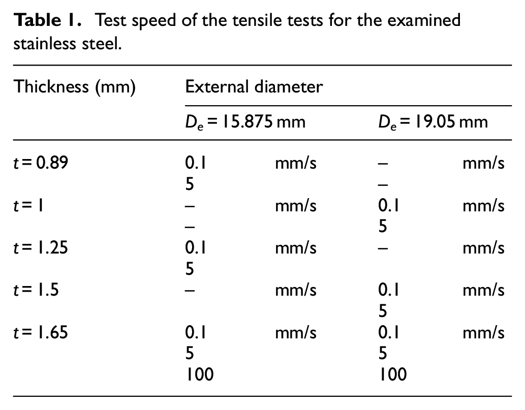
The tests were performed in stroke control until tensile failure occurred. Three loading speeds were examined to study the effects of the strain rate, namely v = 0.1, 5 and 100 mm/s. To prevent the tubes collapse from the compression applied by the grips of the testing machine, a steel plug was introduced into both ends of the samples. This practice is suggested by the test standard ASTM E8M-16a.

The stress–strain curves, tensile strength of the material and strain-rate influence are shown in Figure 1. The material has a moderate strain-rate sensitivity, although the examined strain-rate levels were relatively low but sufficient for the examined application. In any case, the material model used in this work considers the strain-rate sensitivity.

Figure 1.

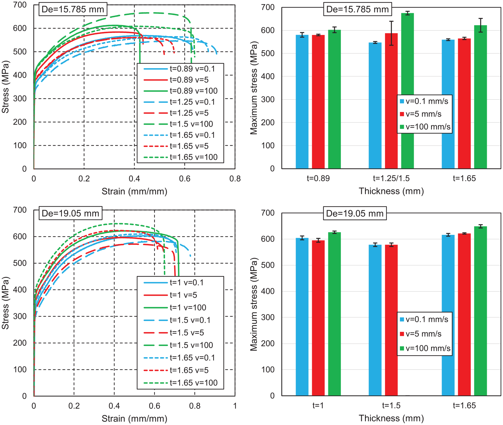
The experimental results of the tensile tests of the analysed stainless-steel tubes as a function of the thickness t, loading speed v and external diameter D_e. The charts on the left side show the stress–strain curve (one curve for each test configuration is shown), and the charts on the right side show the average values and the scatter of the tensile strength.

Driving force

To develop and validate the numerical model, a series of simplified components were considered and studied. Due to the practical impossibility of performing experimental measurements directly on the real components, simplified sub-components were considered to measure the process parameters, particularly the force required to drive the ogive to achieve tube expansion.

Two different test setups were used, namely simple tubes laterally free (unconstrained, without fins, Figure 2) and small-scale heat-exchanger models (Figure 3). These latter models consisted of a pack of fins between simplified end plates. The pack of fins is crossed by seven tubes with the axis perpendicular to the plane of the fins. One tube is positioned in the centre of the fins, whereas the other six tubes are positioned according to a hexagonal pattern. The central tube was subjected to the ogive insertion, while the remaining six had only a supporting function. The distance between the tubes and their positions reflected the standard production proportions. The tubes had standard thicknesses of 1 and 1.5 mm.

Figure 2.

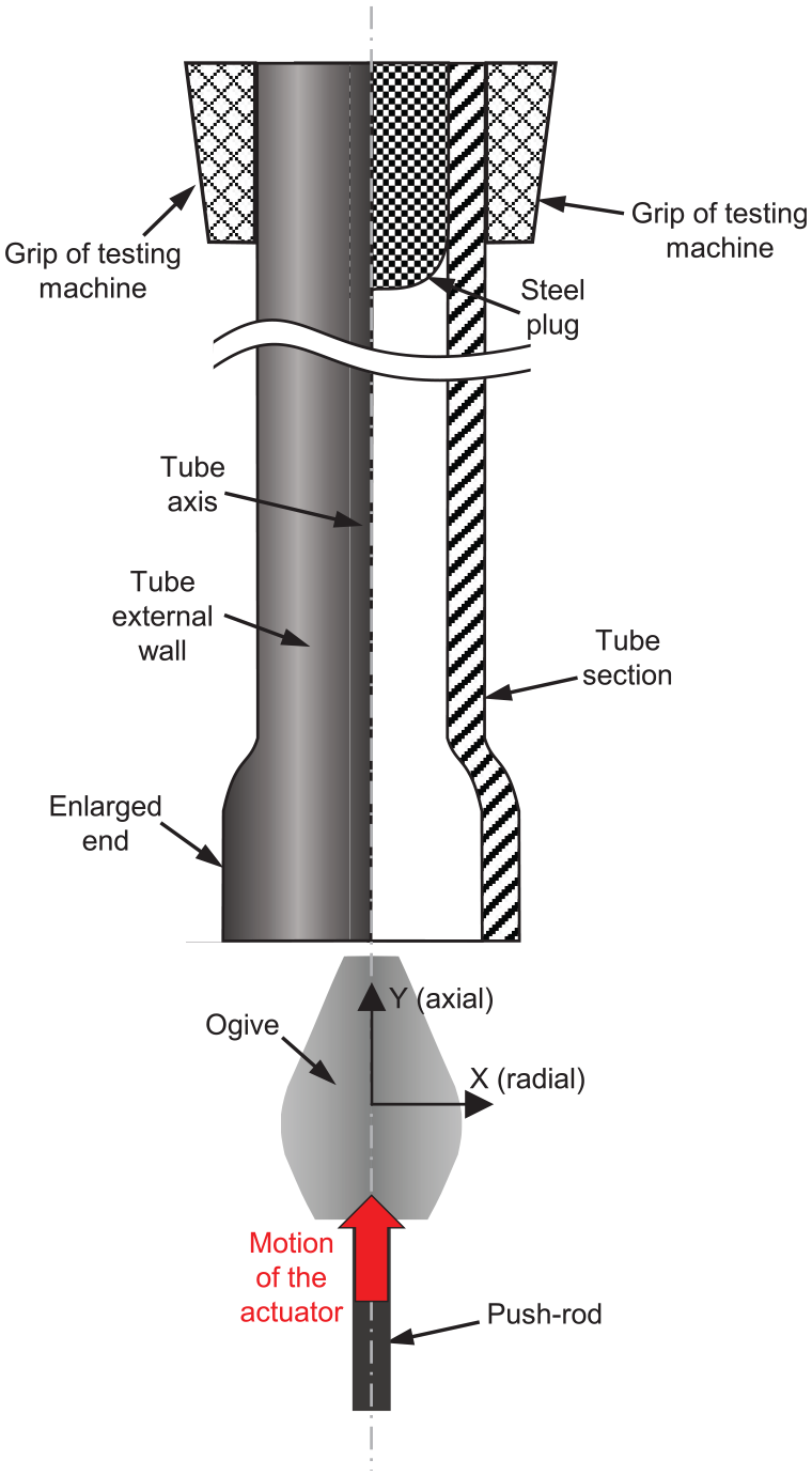
The configuration of the experimental expansion test adopted for the simple, laterally free tubes.

Figure 3.

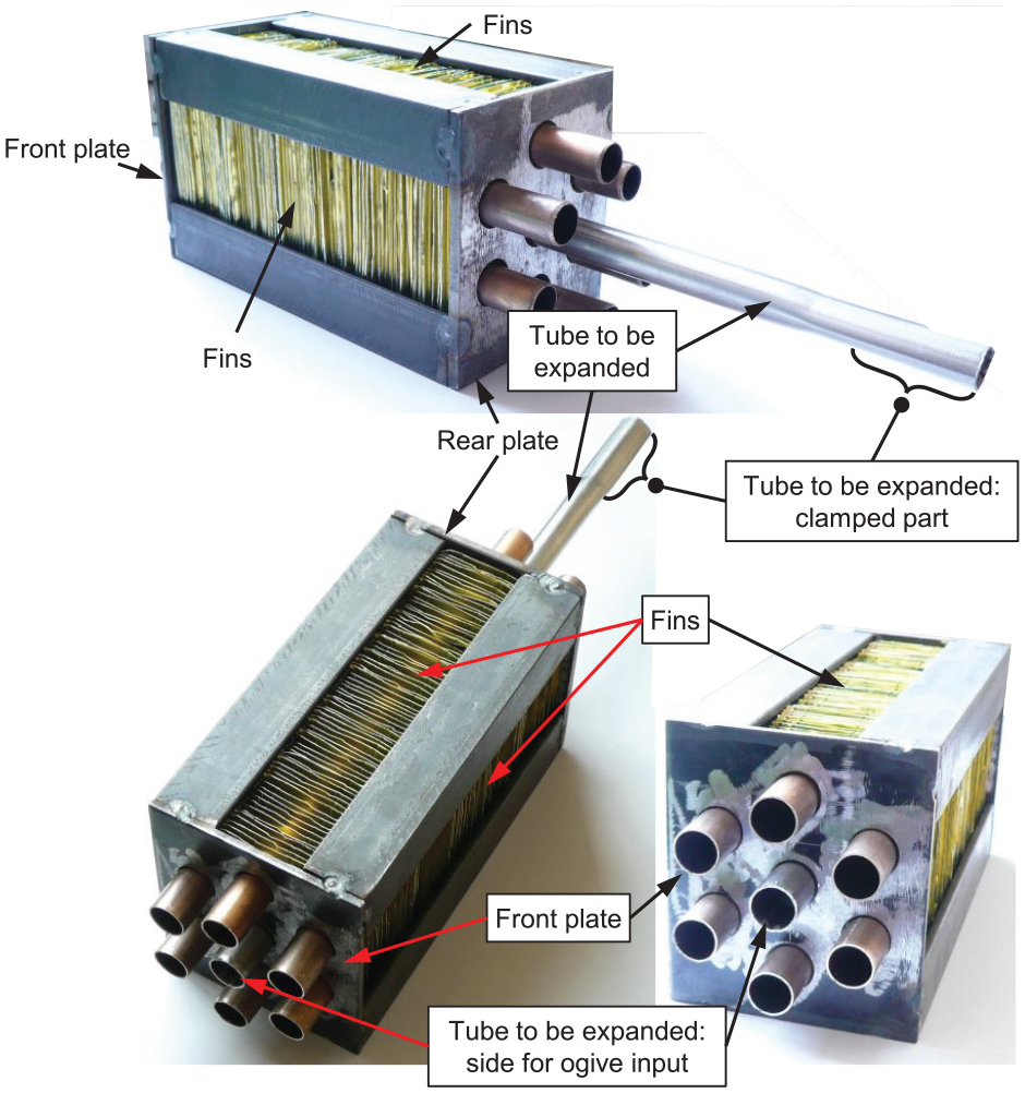
Different views of the small-scale heat-exchanger model used for the expansion tests.

The shape and size of the ogive are shown in Figure 4 and Table 2, respectively. In the case of the tests on the simple, laterally free tubes, the ends were pre-formed to ease the ogive insertion at the beginning of the process (and during production). This pre-forming was applied for the first 10 mm of tube length. One of the ends was clamped in the testing machine, as in Figure 2, while the other was used for the ogive insertion.

Figure 4.

Ogive shape and dimensions.

Table 2.

Ogive dimensions with reference to Figure 4, all the dimensions are in mm.

t	De	R	L	D1	D2	D3
1	15.875	5	11	14.54	6.25	9.67
1.5	19.05	5	11	13.10	6.25	8.23
1	15.875	5	11	17.50	6.25	12.63
1.5	19.05	5	11	16.25	6.25	11.38

During the ogive insertion tests, the driving speed was chosen as 10 mm/s for the simple, laterally free tubes and 100 mm/s for the small-scale heat-exchanger models. This insertion speed value reproduces the typical speed adopted in the manufacturing process. Grease, equivalent to the real production process, was used for proper lubrication between the inner wall of the tube and the ogive. At least three repetitions of each test were conducted.

The experimental results will be shown in section §3.2. A comparison with the results of the numerical models will be also proposed and discussed.

Forming process simulation

Modelling

A series of FE analyses was conducted using the LS-DYNA 971 software, version double precision, release 7, implicit solver option.

Material modelling

The material properties of the tubes were identified by simulating the tensile tests described in section §2.1. Tensile tests on expanded tubes, that is tubes subject to expansion in laterally free conditions, as in Figure 2, were also performed to validate the model.

Several models for the materials from the collection of the used FE software³⁵ were considered and accurately selected. The most suitable model for this application was then considered the elastic visco-plastic material model (MAT_106 of the LS-DYNA collection), as it considers thermal effects. This model is described in equation (1):

\begin{matrix} σ (ε_{eff}^{p}) = σ_{0} + Q_{r 1} [1 - \exp (- C_{r 1} ε_{eff}^{p})] \\ + Q_{r 2} [1 - \exp (- C_{r 2} ε_{eff}^{p})] + \\ + Q_{χ 1} [1 - \exp (- C_{χ 1} ε_{eff}^{p})] \\ + Q_{χ 2} [1 - \exp (- C_{χ 2} ε_{eff}^{p})] \end{matrix}

(1)

Where:

σ₀ yield stress

ε_eff effective plastic strain

Qr_1,2 and Cr_1,2 parameters of isotropic hardening

Qχ_1,2 and Cχ_1,2 parameters of kinematic hardening

The visco-plastic effect is accounted for with the Cowper–Symonds³⁶ model .

Simulations of the tensile tests were carried out for all thicknesses (1 or 1.5 mm) and speeds (0.1, 5 or 100 mm/s). The outcomes of the identification are shown in Figure 5, where the experimental and numerical results are compared.

Figure 5.

Simulation results of the tensile tests: comparison between the experimental results (curves in different grey levels) and the numerical identified curves (in red colour) for specimens with external diameters: (a) D_e = 15.875 mm and (b) D_e = 19.05 mm.

Simulation of the laterally unconstrained simple tube expansion

An axisymmetric model was created in LS-DYNA to simulate the expansion test on the tubes without lateral constraints (Figure 2). This derives from the assumption of perfect axial symmetry of both the tube and the inserted ogive; it is a strong assumption not completely true for the real components but an adequate approximation at the current study level and for practical purposes. Such an analysis was carried out by Scattina²⁷; errors include deviation from the ideal circular cylindrical shape of both the internal and external surfaces (in principle, the section shapes can be approximated by ellipses) and a lack of coaxiality between the two surfaces. The axisymmetric model has the great advantage of a dramatic simplification of the model and a huge reduction in calculation times.

The axisymmetric model consisted of three/four nodes plane axisymmetric elements. The average size of the elements was 0.125 mm. Therefore, the number of elements was between 13 × 10³ and 20 × 10³, depending on thickness. The ogive was modelled with a rigid material and axisymmetric elements. The friction between the ogive and the tube was modelled with a simple sliding model, and the coefficient of friction was chosen as 0.15 from a previous analysis by Avalle et al.² Boundary conditions (Figure 6), to reproduce the real loading conditions, were applied to axial displacements of the first line of nodes of the tube, at the end opposite to that where the ogive was inserted. Then, a constant axial insertion speed of 10 mm/s was applied to the ogive; a sliding interface was used to model the contact between the ogive surface and the internal tube surface.

Figure 6.

The numerical model (on the left-hand side of the figure) used to simulate the unconstrained tube subjected to the expansion test (right-hand side of the figure).

Simulation of the small-scale heat-exchanger models

To consider the effect of the lateral constraint of the fins, the second model was developed to reproduce the small-scale heat-exchanger tests (Figure 7). The model was similar to that of the simple tube, built with axisymmetric elements for the tube section and for the fin section (an average size of 0.075 mm was used for the fin element). The fins are non-axisymmetric, but they were modelled as simple axisymmetric plates exploiting the local nature of the expansion process. The fin plates had a diameter measured at a distance equal to half the tube’s pitch. This diameter was then radially constrained in the model. A further contact algorithm was added between the fins. The aluminium alloy of the fins was modelled as simply bi-linear elasto-plastic material. The material parameters were obtained from previous tests of the authors.²⁷ The end clamped in the testing machine was constrained for a length of 45 mm, as in the experimental setup. The ogive was subjected to a constant axial insertion speed of 100 mm/s, as in the previous model.

Figure 7.

Numerical model (on the left-hand side of the figure) for the simulation of the tube expansion for the heat-exchanger model.

Validation of the numerical models

To validate the FE models used for the simulation of the experimental test of the simplified expansion process, the results are compared, as shown in Figure 8, in terms of the axial driving force of the ogive and, in Table 3, in terms of the tube’s dimensions after expansion. The comparison is excellent for thicknesses of a smaller value, while it is less satisfactory for thicker tubes. From various analyses performed by the authors² and from what can be found in the literature,⁹ the critical role of the friction value can be shown. A slight change in the friction coefficient value between the ogive and the inner wall of the tube could change the value of the axial driving force. This could explain the difference obtained with thicker tubes of a smaller diameter. Moreover, to obtain simple synthetic models of the tube expansion, the approximation was considered sufficient to describe the problem.

Figure 8.

The comparison of the axial driving force of the ogive between the numerical and experimental results for the specimens with external diameter: (a) D_e = 15.875 mm and (b) D_e = 19.05 mm.

Table 3.

Size analysis of tube specimens: comparison between numerical and experimental results after the expansion tests. All dimensions are in mm.

External diameter D_e	Thickness t	External diameter after expansion			Internal diameter after expansion
		Experimental (averaged value)	FEM	Difference	Experimental (averaged value)	FEM	Difference
15.875	1	16.64	16.65	−0.01	14.66	14.70	−0.04
15.875	1.65	16.33	16.46	−0.13	13.15	13.23	−0.07
19.05	1	19.57	19.57	0.00	17.59	17.60	−0.01
19.05	1.65	19.60	19.62	−0.02	16.35	16.38	−0.03

Investigation of the process parameters

To obtain a synthetic model of the expansion process, parametric simulations were performed by varying the values of some mostly significant variables. Processing parameters are countless, but only a few can be considered important and measurable in terms of input/output. Among the process parameters, the following were considered for the synthetic model, based on previous experiences of both the authors and the manufacturers:

the friction coefficient f between the internal surface of the tube and the ogive;

the initial thickness t₀ of the tube;

the insertion speed v of the ogive.

A multilevel factorial design was used to change the three variables according to Table 4; two variables, tube thickness and insertion speed, were considered at three levels, whereas friction was varied at four different levels. Then, the 24 combinations of the three variables were numerically simulated.

Table 4.

The variation in factor levels.

Factor	Levels
Friction coefficient, f	0.15–0.30–0.40–0.60
Insertion speed, v (mm/s)	50–100–150
Tube thickness, t₀ (mm)	1.0–1.25–1.65

For each simulation, the radial and axial components of the driving force of the ogive were obtained as a function of the ogive position. As shown in Figure 9, the axial driving forces increase then stabilise with small variations (less than 2%) in what can be considered a steady-state region, which was conventionally defined for an ogive stroke greater than 20 mm. The mean radial and axial driving forces of the ogive were then calculated as the average in the steady-state region.

Figure 9.

Examples of the axial driving force as a function of the ogive’s stroke obtained in the numerical simulations.

The ratio of the mean radial and the axial components of the ogive driving force does not remain constant but depends on the process parameters. In Figure 10, the value of the mean radial and axial forces are reported as a function of the wall thickness and the insertion speed. The four values of the friction coefficient are also considered. Of course, the mean driving force can also be represented as the value of the mean resultant R and of its angle α measured clockwise with respect to the radial axis, as shown in Figure 11.

Figure 10.

The results for the driving force: (a) axial and (b) radial average components as a function of the process parameters. Transparent surface (top) for diameter D_e = 15.875 mm, shaded (bottom) for diameter D_e = 19.05 mm.

Figure 11.

Numerical results for the driving force: (a) average resultant and (b) angle as a function of the process parameters. Transparent surface (top) for diameter D_e = 15.875 mm, shaded (bottom) for diameter D_e = 19.05 mm.

Another important result from the numerical model is the radial force developed in the contact between each single fin and the tube. In Figure 12, the radial force in the contact is shown. Its variability with the ogive stroke is considered. Five different trends are considered for fins equally spaced along the axis tube. For each fin, the radial force reaches a maximum – when the ogive expands the tube closest to that fin – then, after a small springback due to the bending of the thin wall, it becomes stable at a constant value. This force is due to the residual stresses caused by the plastic deformation of the tube. The radial force remaining on the different fins is not constant; this is due to end effects because in the small-scale heat-exchanger models, the tube length is relatively short with respect to the tube diameter. In longer tubes, as in the real production components, end effects will vanish after a sufficient tube length, and a constant value of the force is expected. However, the variation, measured by the standard deviation of the final remaining radial force, is poor (around 10%), so the average can be considered a good estimate of the force exerted by the tubes on the fins. This average value is examined as follows in Figure 13. In this figure, the values of the average radial force exchanged with the fins are also reported. Variabilities in wall thickness and insertion speed are considered, and the evaluation is repeated for the different friction coefficient values.

Figure 12.

An example showing the variation in radial forces developed in the contact between the tube and the fins. Five different positions in the tube’s axial direction are considered.

Figure 13.

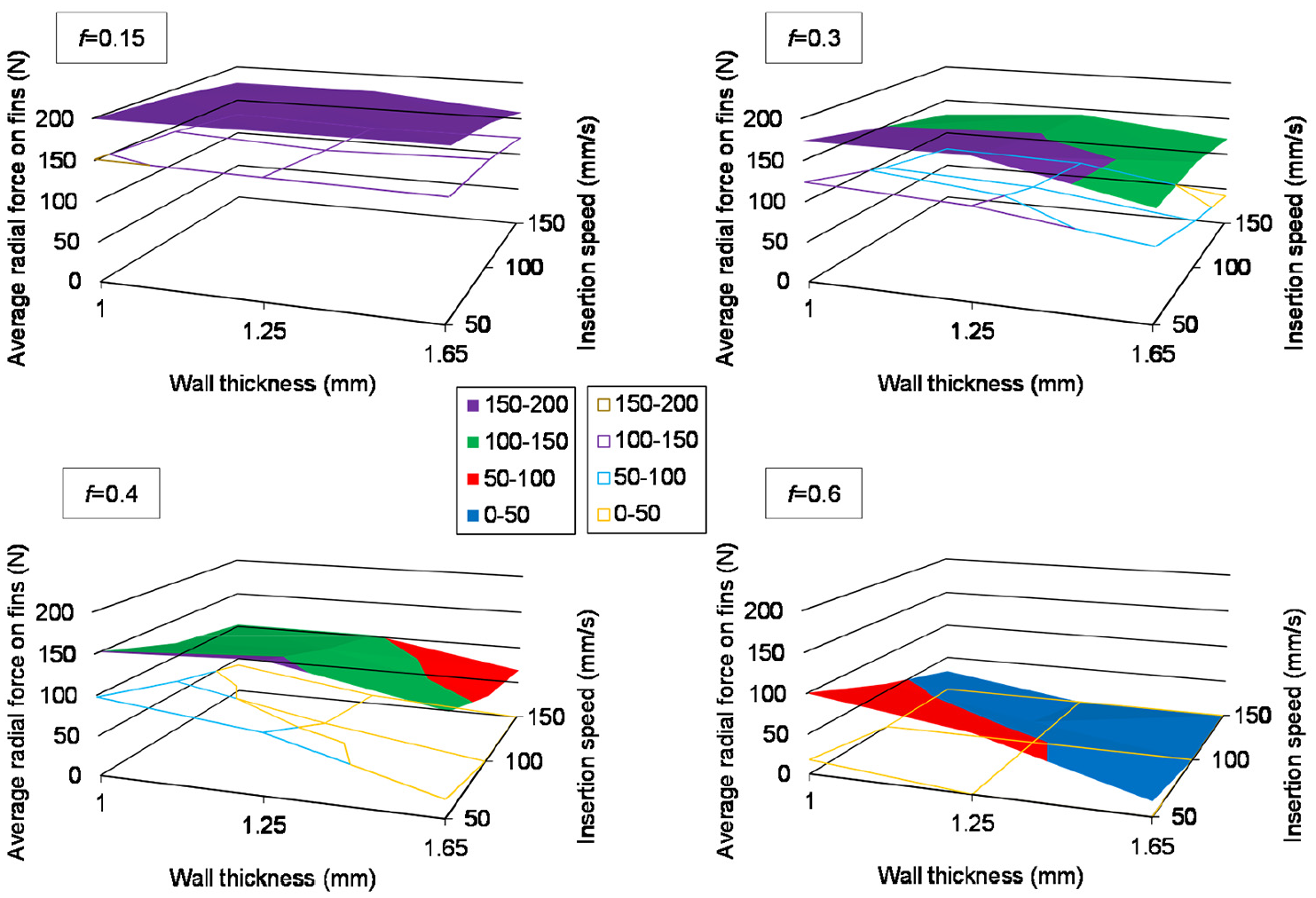
Radial force on the fins: transparent surface (top) for diameter D_e = 15.875 mm, shaded (bottom) for diameter D_e = 19.05 mm.

The final contact area between the tubes and the fins is then the last important outcome of this analysis; the contact is essential for the heat exchange between the (usually warmer) fluid in the tubes and the (usually colder) air passing over the fins. It was observed that – unexpectedly – the contact is incomplete and remains in a highly limited area only, as shown in Figure 14. The fact that the contact area is reduced, at least within reasonable and measurable limits, does not seem to significantly influence the heat exchange from experimental observations; even a small contact area between two materials with high thermal transmissivity generates thermal bridges largely sufficient for heat transmission. The average remaining gap (Figure 15) was then calculated by measuring its value for five fins along the tube and taking the maximum distance between the fin and the tube. The measure was repeated for each fin.

Figure 14.

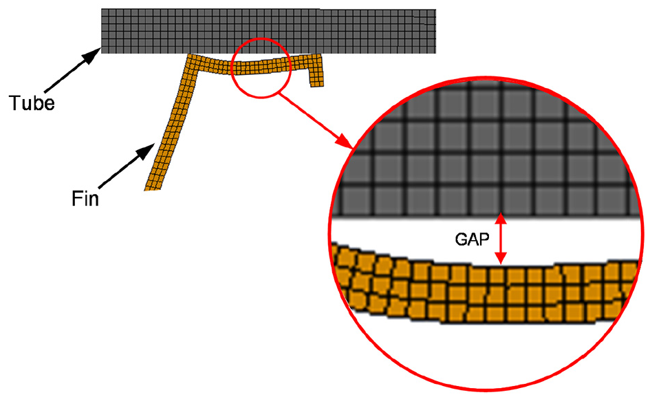
Detail of the contact zone between the tube and the fin after the expansion (the deformation of the fin is enlarged 50 times in the figure) and criterion for the evaluation of the gap measure.

Figure 15.

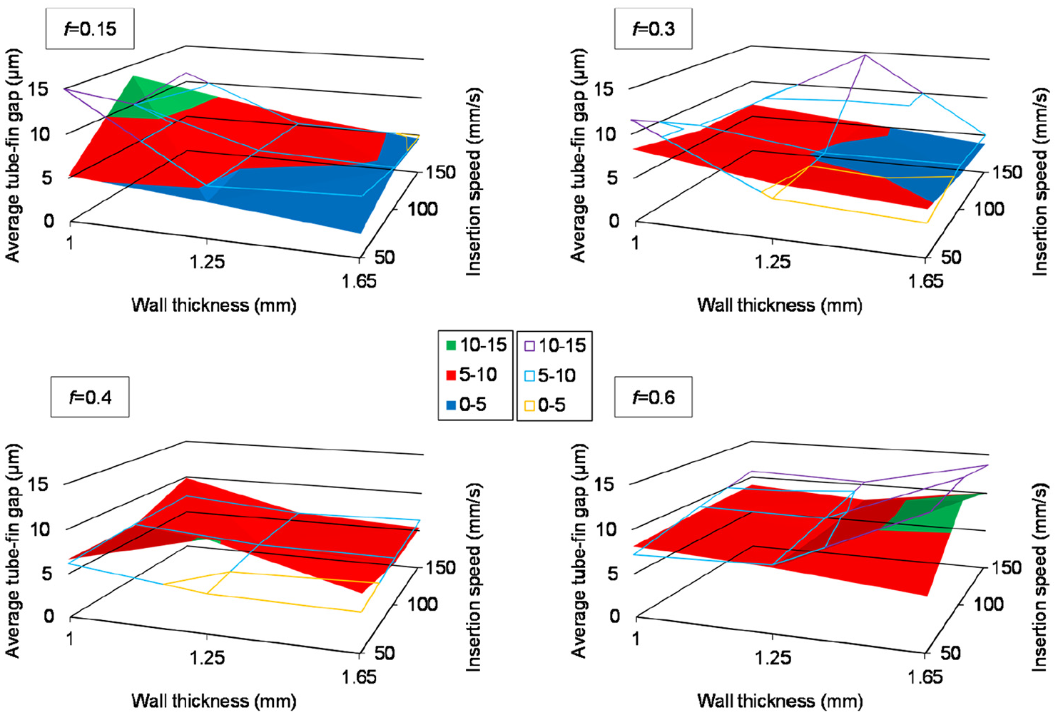
Analysis of the maximum tube–fin gap: transparent surface (top) for diameter D_e = 15.875 mm, shaded (bottom) for diameter D_e = 19.05 mm.

The average values, calculated as a function of the wall thickness and insertion speed, are reported in Figure 15. The evaluation is repeated for the considered values of friction.

Discussion: Analysis of the influence of the process parameters

In the following sections, the influence of the three factors considered in the analysis is discussed based on the numerical model results.

Friction coefficient

From the analysis of the effect of the friction coefficient f (Figure 10), a strong influence on the driving force in the axial direction F_d,a is apparent, whereas the radial force F_d,r is only slightly affected. This confirms the result obtained from CuNi tubes, as reported by Hwang and Altan.³ Consequently, because the radial force is higher than the axial force, the friction coefficient f produces only a slight increase of the resultant R (Figure 11). Increasing the friction coefficient f increases the angle α, and this effect is explained by an increase in the friction force that is backward-oriented in the direction of the ogive motion. Moreover, the expansion of the tube is lower for higher friction, and this effect is explained by an increment of the energy dissipated by the friction forces. Consequently, the outer diameter of the tube D_e (= D_i + 2 t) is subjected to a lower expansion, and the force in the contact between the fins and the tube (Figure 13) is affected as well. Finally, an increase in the maximum gap g_max is observed (Figure 15, on the left) with higher friction.

Insertion speed

The insertion speed v also influences the ogive driving force, but much less than the friction coefficient. The two components (axial and radial) of the driving force (from Figure 10) and the resultant force R (in Figure 11) both increase with the insertion speed, so the angle α remains almost constant. In terms of tube expansion, the insertion speed does not significantly affect the diameter and thickness variations. With higher friction coefficient values, however, a slight decrease in the contact force between the tubes and fins with the insertion speed v is noticeable, independent of the thickness. Instead, the insertion speed v has no significant influence on the gap (Figure 15).

Tube thickness

The numerical model demonstrated that the tube thickness linearly influences the magnitude of both components of the driving force (Figures 10 and 11) and the resultant R, whereas, again, the effect of the angle α is negligible (Figure 11(b)). The average radial force in the contact between the fins and the tube is slightly higher for t = 1.5 mm considering the lowest friction coefficient value (f = 0.15). At higher friction coefficient values (Figure 10), the opposite trend is noticed. The component of force in the radial direction due to friction becomes more important. However, the variation is so small that further investigation seemed unnecessary; analysis of the interactions revealed a negligible correlation between these parameters. Finally, the maximum gap between the tube and fin is reduced by increasing the thickness (Figure 15).

Conclusions

A detailed analysis of the mechanical process of stainless-steel tube expansion was performed. This process is used to produce air heat-exchangers with finned tubes. The analysis was based on the results of experimental tests on the material and on the process, as well as of subsequent simulations. First, the parameters of a suitable material model were obtained using the experimental results. The same data were then used to validate a numerical model of the tube expansion process. The models were based on the assumptions of axial symmetry, allowing for reduced 2D FE analyses. Such a simplified model was, however, adequate for a correct description of the analysed problem. A good agreement between the numerical results – in terms of driving forces in the radial and axial directions – and the experimental data was revealed. The evaluation of the axial driving force is the main process parameter, as it is related to the power required for the process and therefore to the manufacturing costs.

A main outcome obtained concerns the effect of the main manufacturing and process parameters, namely tube geometry, insertion speed and friction, on the driving force. In addition, the model can give indications of the characteristics of the contact between the tubes and the fins. From the reported analysis, it appears that friction is the main influencing factor; to reduce the driving force, it is necessary to reduce friction. Lubrication is essential to reduce the power and energy required for tube expansion, as well as to, as it appeared, improve the contact between the tubes and the fins by reducing the gap between these two parts.

Therefore, the model can be considered an important tool to predict the process and product performance of finned tube air heat-exchangers and could be a useful basis for the optimisation of the production process.

Footnotes

Acknowledgements

Astra Refrigeranti S.r.l cooperated in this research activity. The authors kindly acknowledge their technical contribution.

Declaration of conflicting interests

The author(s) declared no potential conflicts of interest with respect to the research, authorship, and/or publication of this article.

Funding

The author(s) received no financial support for the research, authorship, and/or publication of this article.

ORCID iD

Alessandro Scattina

References

MacGregor

Coffin

Fisher

. The plastic flow of thick-walled tubes with large strains. J Appl Phys 1948; 19(3): 291–297.

Avalle

Priarone

Scattina

. Experimental and numerical characterization of a mechanical expansion process for thin-walled tubes. J Mater Process Technol 2014; 214(5): 1143–1152.

Hwang

Altan

. Finite element analysis of tube hydroforming processes in a rectangular die. Finite Elem Anal Des 2003; 39: 1071–1082.

Abrantes

Szabo-Ponce

Batalha

. Experimental and numerical simulation of tube hydroforming (THF). J Mater Process Technol 2005; 164–165: 1140–1147.

Gao

Strano

. FEM analysis of tube pre-bending and hydroforming. J Mater Process Technol 2004; 151: 294–297.

Ray

MacDonald

. Determination of the optimal load path for tube hydroforming processes using a fuzzy load control algorithm and finite element analysis. Finite Elem Anal Des 2004; 41: 173–192.

Tan

Yao

Zhang

, et al. Thermo-mechanical coupling analysis of expansion tubes: theoretical prediction and experimental investigation. Thin-Walled Struct 2021; 162: 107559.

Zhang

. A new model for the expansion tube considering the stress coupling: theory, experiments and simulations. Def Technol. Epub ahead of print 20 May 2021. DOI: 10.1016/j.dt.2021.05.010.

Luo

Yang

Liu

, et al. Energy absorption of expansion tubes using a conical-cylindrical die: theoretical model. Int J Mech Sci 2019; 157–158: 207–220.

10.

Liu

Qiu

. A theoretical study of the expansion metal tubes. Int J Mech Sci 2016; 114: 157–165.

11.

Yang

Luo

Hua

, et al. Energy absorption of expansion tubes using a conical–cylindrical die: experiments and numerical simulation. Int J Mech Sci 2010; 52: 716–725.

12.

Hwang

Chen

. Analysis and finite element simulation of tube expansion in a rectangular cross-sectional die. Proc IMechE, Part B: J Engineering Manufacture 2003; 217(1): 127–135.

13.

Pervez

Seibi

Karrech

. Simulation of solid tubular expansion in well drilling using finite element method. Pet Sci Technol 2005; 23(7–8): 775–794.

14.

Pervez

Qamar

Al-Abri

, et al. Experimental and numerical simulation of in-situ tube expansion for deep gas wells. Mater Manuf Process 2012; 27(7): 727–732.

15.

Seibi

Barsoum

Molki

. Experimental and numerical study of expanded aluminum and steel tubes. Procedia Eng 2011; 10: 3049–3055.

16.

Seibi

Al-Hiddabi

Pervez

. Structural behavior of a solid tubular under large radial plastic expansion. J Energy Resour Technol 2005; 127(4): 323–327.

17.

Seibi

Pervez

Al-Hiddabi

, et al. Finite element modeling of a solid tubular expansion – a typical well engineering application. Society of Petroleum Engineers (SPE) Technical paper, SPE84943, 2005.

18.

Alves

Afonso

Martins

. A new deformation assisted tube-to-tubesheet joining process. Thin-Walled Struct 2021; 163: 107784.

19.

Bouzid

Zhu

. A study of neighbouring tube expansion effect on the residual contact pressure of tube-to-tubesheet joints. Int J Press Vessel Piping 2018; 165: 185–192.

20.

Bouzid

Pourreza

. Analysis of residual stresses in the transition zone of tube-to-tubesheet joints. J Press Vessel Technol 2019; 141(4): 1201–1211.

21.

Bouzid

Kazeminia

. Effect of reverse yielding on the residual contact pressure in tube-to-tubesheet joints. J Press Vessel Technol 2016; 138(6): 1402–1410.

22.

Tang

Peng

. An experimental and numerical study of the expansion forming of a thick-walled microgroove tube. Proc IMechE, Part C: J Mechanical Engineering Science 2009; 223: 689–697.

23.

Tang

Peng

. Numerical and experimental study on expansion forming of inner grooved tube. J Mater Process Technol 2009; 209: 4668–4674.

24.

Tang

Peng

. Optimization to the tube–fin contact status of the tube expansion process. J Mater Process Technol 2011; 211: 573–577.

25.

Kwon

Kim

Han

, et al. A new methodology for detecting adhesion location in aluminum tube expansion. Adv Mech Eng 2017; 9(11): 1–8.

26.

Kang

Son

, et al. Three-dimensional fin-tube expansion process to achieve high heat transfer efficiency in heat exchangers. J Mech Sci Technol 2019; 33: 4401–4406.

27.

Scattina

. Numerical analysis of tube expansion process for heat exchangers production. Int J Mech Sci 2016; 118: 268–282.

28.

Karrech

Seibi

. Analytical model for the expansion of tubes under tension. J Mater Process Technol 2010; 210: 356–362.

29.

Alves

Gouveia

BPP

Rosa

PAR

, et al. On the analysis of the expansion and reduction of thin-walled tubes using a die. Proc IMechE, Part B: J Engineering Manufacture 2006; 220(6): 823–835.

30.

Alves

Silva

Nielsen

, et al. Pressure-assisted forming of non-concentric tubular cross sections with solid medium. Proc IMechE, Part B: J Engineering Manufacture 2017; 231(12): 2123–2132.

31.

Gouveia

BPP

Alves

Rosa

PAR

, et al. End forming of thin-walled tubes using a die. Int J Mechatron Manuf Syst 2008; 1(2–3): 183–194.

32.

Mack

. The effect of tubular expansion on the mechanical properties and performance of selected octg – results of laboratory studies. In: Offshore technology conference, Houston, TX, 2–5 May 2005.

33.

Avalle

Scattina

. Experiment based modeling of the mechanical expansion of tubes for the construction of heat exchangers. Procedia Struct Integr 2018; 12: 130–144.

34.

Han

Sin

Kwon

, et al. The role of the process and design variables in improving the performance of heat exchanger tube expansion. Appl Sci 2018; 8: 756.

35.

LS-DYNA keyword user’s manual version 971. Livermore, CA: Livermore Software Technology Corporation (LSTC), 2015.

36.

Cowper

Symonds

. Strain hardening and strain rate effect in the impact loading of cantilever beams. Report, Brown University, Division of Applied Mathematics. Report no. 28, 1957.

Analysis of the mechanical expansion process of thin-walled tubes for air heat-exchanger production

Abstract

Keywords

Introduction

Experimental characterisation: Material properties and driving force

Material properties

Driving force

Forming process simulation

Modelling

Material modelling

Simulation of the laterally unconstrained simple tube expansion

Simulation of the small-scale heat-exchanger models

Validation of the numerical models

Investigation of the process parameters

Discussion: Analysis of the influence of the process parameters

Friction coefficient

Insertion speed

Tube thickness

Conclusions

Footnotes

Acknowledgements

Declaration of conflicting interests

Funding

ORCID iD

References