
Abstract
A novel prognostic approach was developed and applied to a machine tool hydraulic unit. Three components were considered: pump, sensor and valve. The proposed methodology exploited a digital twin of the system to perform simulations of the healthy and faulty machine. The digital twin was properly validated through experiments. This approach dealt with the need to carry out time-consuming and expensive experimental campaigns, that is, run-to-failures – not affordable in many industrial applications. The diagnosis module was trained on digital twin simulations and fulfilled the fault detection, isolation and quantification phases. The challenge related to the variability of the operating conditions of the machine was addressed through a robustness analysis of the methodology. The solution successfully dealt with both stationary and non-stationary working conditions. A dedicated classification model was designed for each faulty component, maximising the associated classification rate. The testing procedure consisted of the application of a 10-fold cross-validation to compute the mean classification rates for stationary and non-stationary working conditions. Diagnosis performance results were excellent for the pump, whereas they were lower for the sensor and valve, reaching 79.75% and 74.93% accuracy respectively for the most challenging working cycle. The prognosis directly exploited the output of diagnostics, allowing for experimental effort reduction. Prognosis predictions were built starting from the updated health status provided by the diagnosis output. In order to test the prognosis module, mean and standard deviation of the prediction errors (less than 1.176%) were computed through a Monte Carlo approach. The conceived methodology allowed one of the critical goals of prognostics to be handled: the Remaining Useful Life probability density function estimation.
Introduction
In manufacturing systems, productivity targets are demanding to ensure maximum reliability and availability of machine tools, 1 while breakdowns and failures need to be fully avoided.2,3 Due to these requirements and increased system complexity, preventive maintenance represents a conspicuous fraction of the total costs in an industrial scenario. 4 Consequently, the attractiveness of Prognostics and Health Management (PHM) solutions rises.
International standards describe the PHM framework5–9 that consists of four modules: preliminary analysis, profile monitoring, diagnosis and prognosis. 10 The first regards the collection and investigation of all possible faults of the analysed system. The second performs the fault detection, that is, the observation of a statistical discrepancy between the ongoing and a pre-recorded healthy working condition. The third deals with fault isolation and quantification, that is, the localisation of the faulty component and its wear level assessment, respectively. The last step deals with the prediction of the Remaining Useful Life (RUL) of the component, that is, the remaining time for which the component can perform the assigned task. RUL estimation should also contain information about its uncertainty through the estimation of its probability density function (pdf). 10
Two steps are needed to create a proper dataset for PHM strategies: feature extraction and feature selection. The first consists of the computation of statistical quantities from sensor data. It enables dimensionality reduction of collected data, trying to condense the information as much as possible. Features can be computed in many domains: time, frequency and time-frequency domain.4,11,12 Feature selection allows for a further reduction of the features pool. Spearman’s and Pearson’s correlation coefficients can be used to rank features and keep the most correlated ones.11,12 ANOVA could be applied when data are collected in classes. 13
Once the dataset is created, profile monitoring techniques can be adopted. Statistical Process Control (SPC) 14 is the typical tool, as proposed by Liu et al. 15 and Colosimo et al. 16
Diagnosis is a classification problem. Several types of algorithms could be used to localise and identify the nature of the fault: Linear Discriminant Analysis (LDA), Support Vector Machines (SVM), 17 Mahalanobis-Taguchi Systems, 18 filtering techniques, for example, Unscented Kalman Filter (UKF) 19 and Artificial Neural Networks (ANN) are just a subset of possible solutions.11,20,21 An innovation in this field could be progressive learning, introducing the capability of increasing the number of clusters during online learning. 22 Additionally, utility theory can be applied to introduce probabilities of critical conditions. It was successfully implemented to support decision making in maintenance actions on bearing faults in a sewage treatment plant. 17
Dealing with prognostics, four main algorithm categories can be distinguished depending on the data availability and the approach to the problem10,23:
Knowledge-based models: expert knowledge is translated in simple rules that the system can interpret. Such methods can be used only if robust knowledge of the degradation phenomenon and the machine is available. Expert systems, in which rules assume the form of IF-THEN, and fuzzy logic, giving a linguistic description of the system, are part of this category10,23;
White-box models (model-based): they rely on a physical model of the degradation phenomenon. 23 Although the model structure is known a priori, experimental data are necessary to identify the model parameters. 10 Exponential lifetime prediction model for ball screw mechanisms under different feed modes, 24 differential models for tool wear evolution in milling 25 and wear model for flank wear in turning 26 are just examples of this;
Grey-box models (statistical-based methods): they rely on a dynamic stochastic description of the degradation phenomenon. The model is selected by the user and its coefficients are estimated through experimental data. 10 Their advantage is related to a statistical description of the RUL and, indeed, a strong support for decision making on maintenance actions. Filtering-based approaches such as Kalman filters 27 and its variations, 28 or particle filters29,30 are all examples of grey-box approaches, as well as Hidden Markov Models (HMM) and Hidden semi-Markov Models. 10 Linear regression models can even be applied for RUL prediction. 31
Black-box models (data-driven): they ‘learn’ and describe the problem directly from the collected data. Data quantity and quality of both faulty and fault-free data are of fundamental importance for successful implementation. 5 ANN, Self-Organising-Maps (SOM)15,32,33 and deep learning algorithms, SVM and Relevance Vector Machines (RVM) 34 are just a few examples of artificial intelligence techniques.
Hybrid approaches have recently emerged, fusing multiple areas and exploiting their synergies. For instance, Sbarufatti et al. 35 developed a prognostic solution for Li-ion batteries using particle filters to update Radial Basis Function Neural Networks. This solution could predict the RUL pdf, providing adaptiveness to new data.
Actually, different challenges prevent PHM techniques to find a robust implementation in manufacturing:
the system under analysis needs to be sensorised to provide meaningful signals regarding the fault conditions. No rules have been designed to choose the right ones;
experimentation is needed: all the techniques available nowadays require training data (data from all the fault combinations or run-to-failures). Typically, only fault-free data are largely available and experimentation can be extremely expensive and time-consuming;
developed solutions are often working-cycle dependent. This is a critical problem in many applications, for example, with machining centres;
how to estimate and deal with the uncertainty of the RUL prediction, that is, the determination of its pdf.
Furthermore, scientific research is still lacking in the manufacturing field. The hydraulic unit is one of the most critical parts and the cause of unexpected breakdowns and downtimes.1,3 From a reliability analysis of 10 CNC lathes from 2009 to 2014, the hydraulic subsystem showed the highest failure rate (22.9% of the total failures). 1 A similar project on 12 machining centres between 2005 and 2010 confirmed the result. 36 Two other contributions highlighted the necessities of performing PHM on machine tool auxiliaries, being sources of unexpected downtimes and of comparable loss of production costs with respect to machine tool main components.37,38 Despite the above, research on PHM of CNC machines is rare in such subsystems, especially on hydraulic units. A case study on monitoring the filter’s health state in an oil mist separator was recently presented in 2019. 37 Authors trained machine learning on healthy data to model the environmental effects on the measured fan power. The reconstruction error was used as the health index (HI) of the filter. Instead, PHM in the machine tools field mainly focuses on tool monitoring and prognostics. Specific force coefficients were addressed as cutting-condition independent and tool-wear sensitive features by Nouri et al. 39 Cheng et al. 40 proposed a machine learning methodology based on cutting forces, vibration signals and machined surfaces’ image features, typically used separately, to monitor the wear of different turning tools over various materials and cutting conditions. McLeay et al. applied a Mahalanobis distance-based unsupervised algorithm to detect anomalies in the cutting process to assess the tool life in milling applications under fixed working conditions. The advantage of being an unsupervised method relies on the fact that only the normality condition is experimented for the training phase. 41 da Silva et al. 42 investigated tool wear evolution in the drilling of high-strength compacted graphite cast irons and individuated the spindle current signal as the best cost-benefit monitoring variable for tool wear. HMM were also applied in different fashions for tool wear applications.43,44 Other subsystems are investigated by research literature to a lesser extent, such as those of the spindle and feed-drive. Chen et al. developed an overall machine tool monitoring method based on the frequency analysis of energy, intended as the collection of power, thermal, current and vibration measurements. Analytical modelling of screw, guide rail and bearing frequencies allowed the health status of the components to be estimated. 45 Moore et al. 46 presented a test scenario in which machine learning and deep learning classifiers were applied for machining defects and machine tool failure-mode classification. Besides this, unsupervised algorithms for clustering were tested for novel failure-mode recognition. Xia et al. developed a diagnosis solution for multiple units of flexible production line machining centres, including feed axes, spindles and converters. A neural network scheme was adapted to each machining centre to avoid the combination explosion of learning rules and miss-classification. 47 Multiple polynomial regression, 48 the Mahalanobis-Taguchi System 49 and SOM 30 were applied to predict the RUL of rolling element bearing failures in the spindle system. Feed-drive system health and its influence on tool wear was investigated through a long-term operational modal analysis of vibration signals. 50
The focus of this paper is mainly concentrated on the challenges mentioned above. A novel approach to deal with PHM was presented, trying to avoid run-to-failures through the use of a Dymola model of the hydraulic unit of a machine tool. In section Materials, the system and the model were described, together with its validation. The proposed solution was explained in section Methods, supported by a graphical representation of the whole approach. Starting from the simulation of different working regimes (subsection Synthetic data generation), the creation of the datasets was described in subsection Feature extraction. The novel structure of the diagnostics phase, exploiting different algorithms for any component, was presented in subsection Diagnostics. In subsection Prognostics, the innovative developed prognosis algorithm was presented, being set free from run-to-failures. Lastly, in section Result, a critical analysis of the entire process was carried out, while future developments and conclusions were reported in section Conclusions.
Materials
System and model description
The system is the hydraulic unit of Mandelli’s Spark machining centres. It is constituted by a high pressure (HP) sub-unit (that drives the tool clamping system and the braking system); a medium pressure sub-unit (that cools down and lubricates the biggest organs in the machine); a low pressure sub-unit (that cools down the oil by pumping it to the chiller).
One of the novelties at the basis of this research was to reproduce the faulty behaviour of the system through simulations. All the described sub-units were modelled together with different fault states of the system. A schematic representation of the digital twin developed in Dymola was shown in Figure 1.
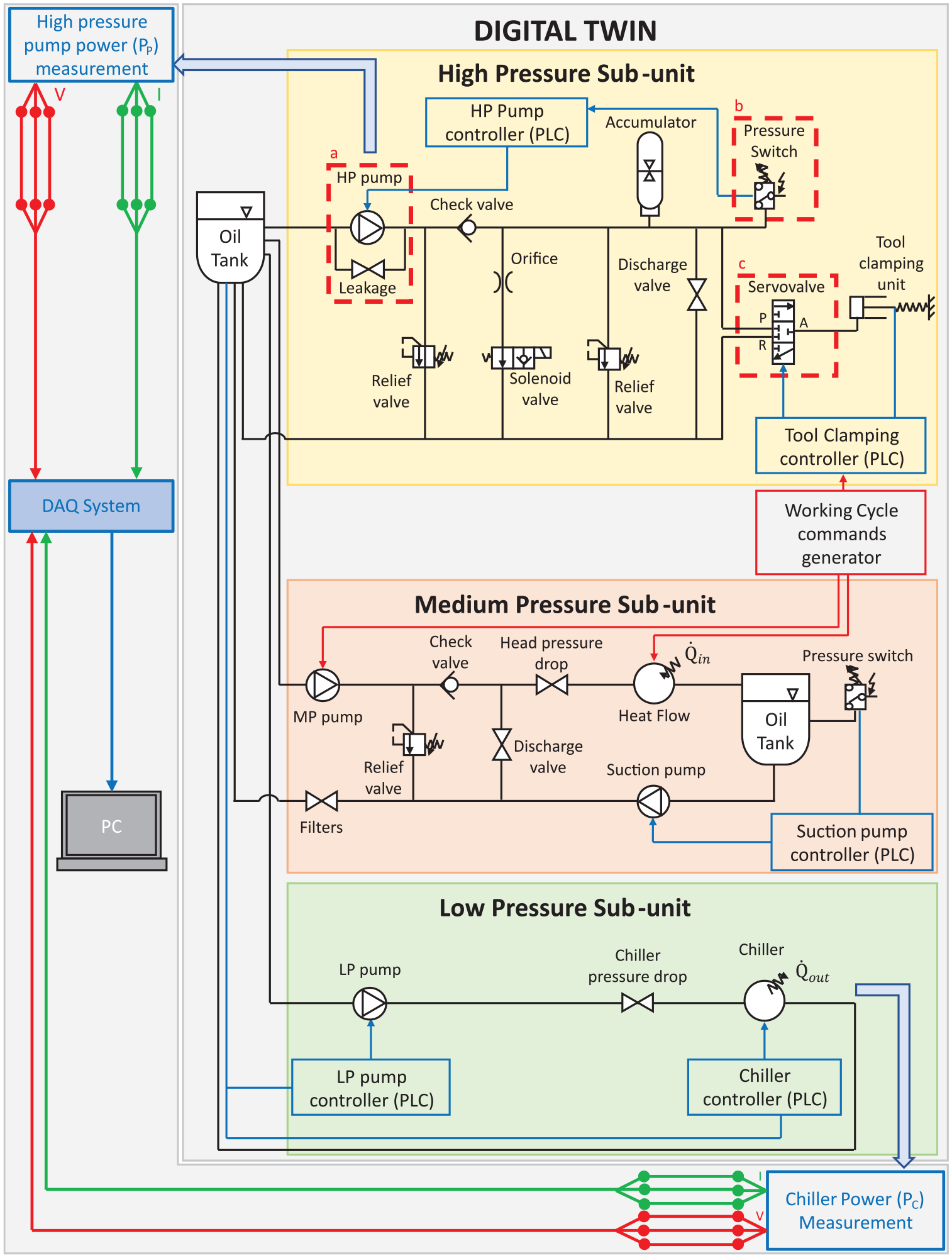
Digital twin layout. Top-left and bottom right arrows represent the link from the digital twin to the measurement system. In the three dashed boxes, the components under analysis: (a) HP pump, (b) pressure-switch and (c) servovalve.
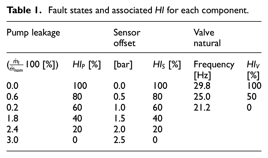
In order to focus only on relevant faults, the history of 15 years of maintenance reports was analysed. They contained data from several similar machines and different faults. The evolution of the fault occurrences over the 15 years was shown in Figure 2. Although filter faults were the ones that occurred the most, they were typically subject to ordinary maintenance. Then, pump, sensor and valve faults were the most frequent and relevant ones. A HP pump leakage (Figure 1(a)), a pressure-switch offset (Figure 1(b)) and an increased opening time for the servo-valve of the tool clamping actuators (Figure 1(c)) were introduced in the model of the system.11,51 The pump was a positive displacement VIVOIL XV1/P-4.9D. The sensor, the subject of the analysis, was a pressure-switch used to keep the HP system between 85 and 95 bar. The HP pump was controlled in a closed-loop by this sensor (IFM PN7071 025-MPa).
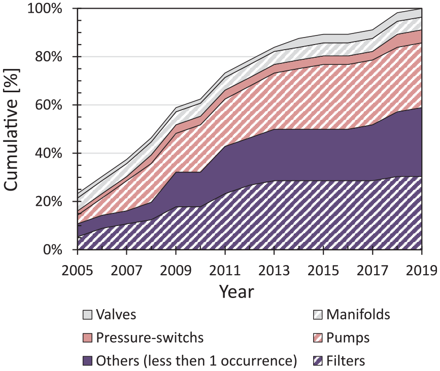
Evolution of fault occurrences over the 15 years maintenance reports.
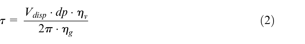
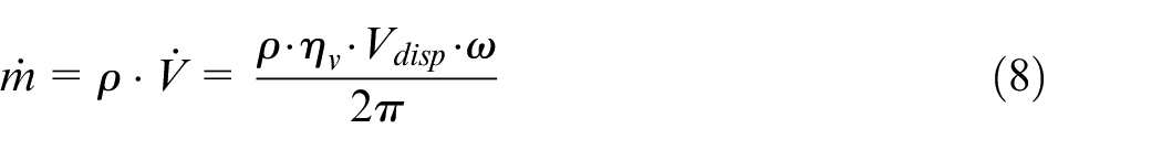
The HP pump was modelled through the following equations:
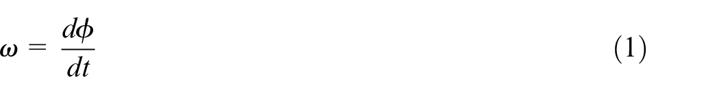
where

where


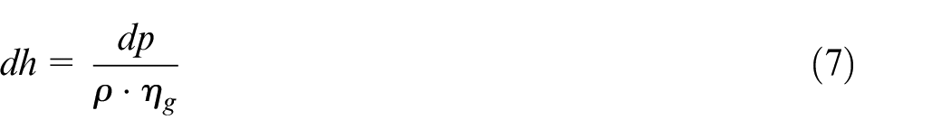
where

The pump leakage was introduced in the model as a valve described by the following equations:


where
Since the pressure switch is a sensor, its output is just the pressure of the oil at the inlet port. It commands the HP pump through an on/off switch. It turns on the pump when the pressure decreases below the lower threshold
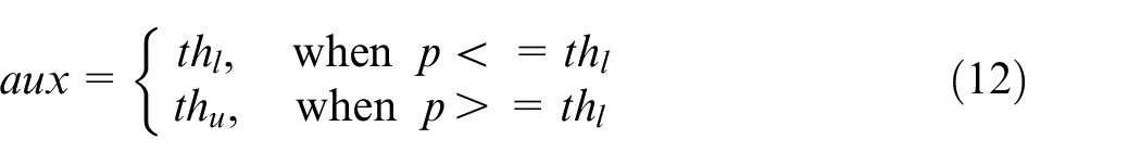
where
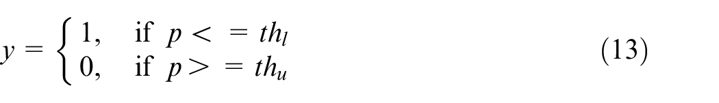
If
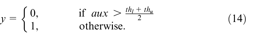
The pressure switch offset was introduced by adding a bias to the real pressure of the system, so that:

where
The servovalve was modelled as two separated valves with complementary opening positions. The first one linked the HP port


where
Fault states and associated
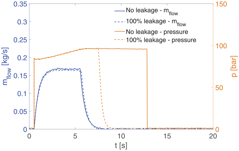
Comparison between pressures and mass flows of the HP pump with and without leakage fault.
Digital twin experimental validation
The validation of the digital twin was conducted by means of power acquisitions performed on a Mandelli’s Spark 1600 machining centre:
power absorbed by the HP pump electric motor;
power absorbed by the chiller;
The experimental setup (Figure 4) was composed of a three-phase acquisition system for phase voltages and currents for each of the above units. Six LEM LF 205-S/SP3 and three NI9205 acquisition cards from National Instruments were adopted.
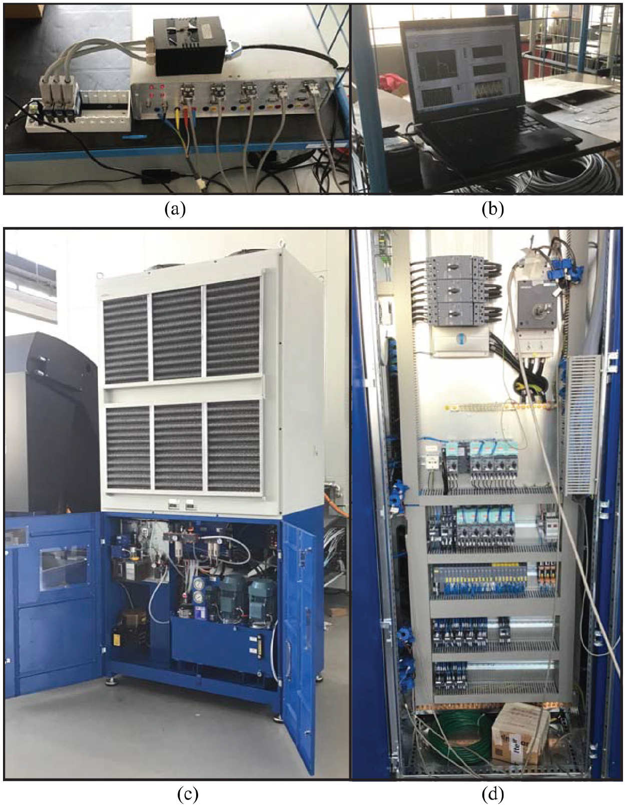
The entire experimental setup: (a) DAQ system and power metre, (b) LabView® acquisition software, (c) hydraulic unit and (d) electrical cabinet and LEM installation.
A brief comparison between the experimental and the simulated physical quantities during a healthy cycle was shown in Figure 5(a). Both the duty cycle and power consumption of the HP pump were respected during the idle time. The validation of the duty cycle and power consumption of the chiller was reported both for the machine warm-up phase (the spindle is activated to reach a steady-state thermal condition, Figure 5(b)) and idle state (Figure 5(c)).
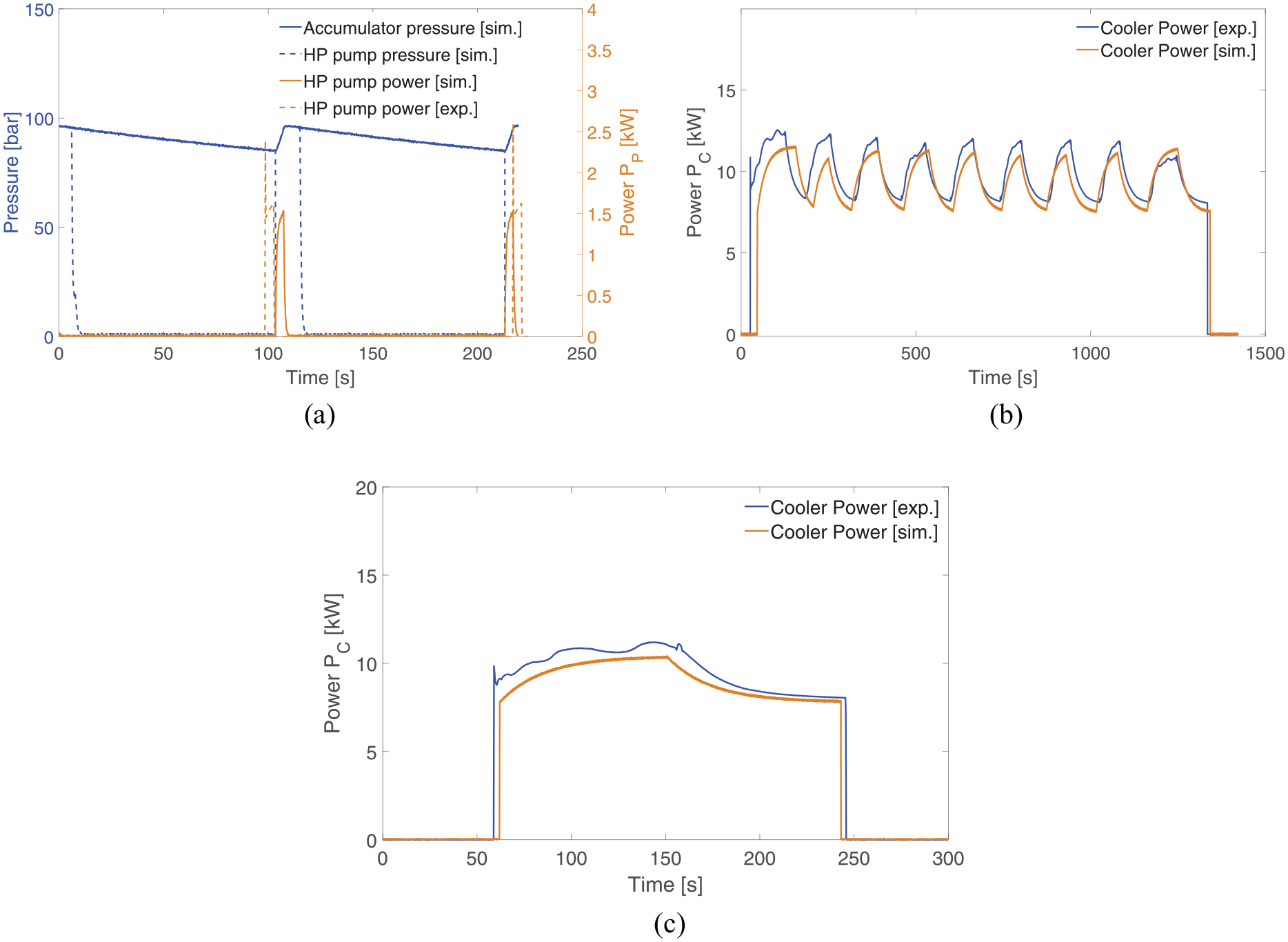
Comparison between experimental and simulated power: (a) acquisitions from HP pump of the unit during a healthy behaviour, (b) acquisitions from chiller healthy behaviour in warm-up and (c) acquisitions from chiller healthy behaviour in idle state.
Methods
Synthetic data generation
In the machine tools scenario, collecting fault data could be a difficult task, perhaps infeasible. A digital twin of the system was used to recreate all possible combinations of fault states (Figure 6(a)) for the components under analysis while operating under different working regimes (Figure 6(b)), following scientific literature53–58 and analogously to what Helwig et al.11,12,51 did experimentally. Indeed, in industrial scenarios, machine tools present high flexibility in working conditions. Hydraulic unit working cycles depend on various parameters such as the occurrence of tool changes, the duration of the machining operations and the loading condition (i.e. the heat transferred to the oil from the machine head/spindle during the operation). It is assumed that a single working cycle for PHM could be acceptable when the machine is dedicated to a single task (e.g. in mass-production industries), while this is not the case for most manufacturing companies. Different working regimes can cause dramatic changes in sensor outputs and, as a consequence, in the classification accuracy. 11
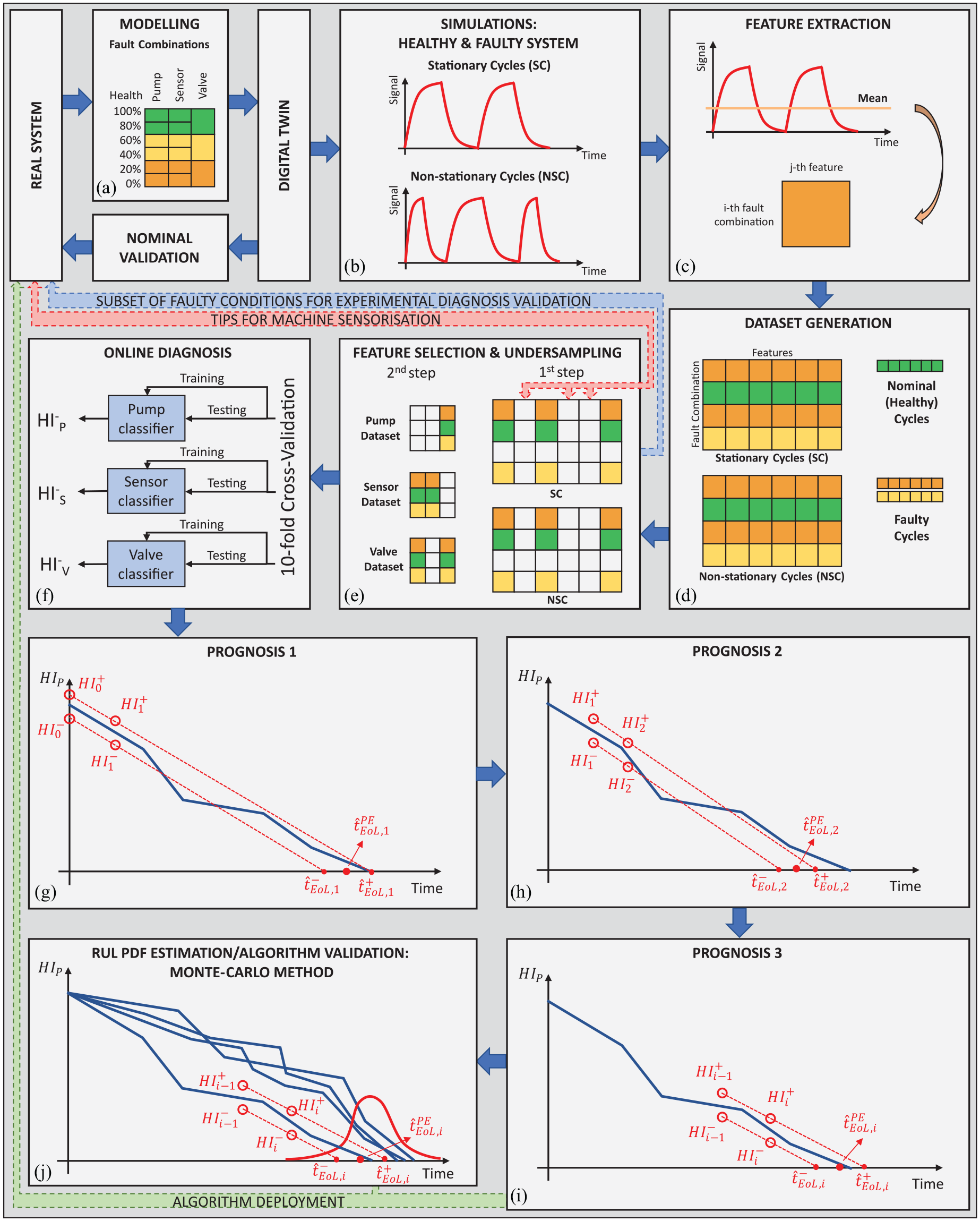
Framework of the whole apporach: (a) modelling of three component faults and associated severities, (b) digital twin simulations of stationary (SC) and non-stationary (NSC) cycles, (c) feature extraction on each fault-combination in SC and NSC, (d) features assembly in SC and NSC datasets, (e) two-step feature selection through one-way-ANOVA scores and undersampling, (f) data-driven diagnosis algorithms training (on SC) and testing (SC and NSC) through 10-fold cross-validation, (g-h-i) iteration steps of the proposed prognostics solution by linear interpolation of online diagnosis output changes, and (j) Remaining Useful Life probability density function estimation by Monte-Carlo sampling.
Then, as a novelty with respect to typical literature approaches, two kinds of working cycles were simulated to test the robustness of the proposed solution: stationary and non-stationary ones, which represented a machine conceived for a specific and a more flexible task, respectively (Figure 6(b)). Non-stationary cycles were created by mixing stationary cycles in fixed proportions, representing more realistic scenarios for a machine tool. Two stationary (SC1 and SC2) and two non-stationary working cycles (NSC1 and NSC2) were simulated:
SC1 was composed of 300 s of machining (tool clamped) and 15 s for tool change (tool released), Figure 7(a). The loading condition was represented by the average heat flow of 5 kW removed from the head/spindle. This cycle comprised stationary subsequent phases of machining and tool changes;
SC2 was composed of 150 and 10 s phases respectively (Figure 7(b)). The average heat flow absorbed by the oil was 3 kW.
NSC1 was composed of 70% of SC1 and 30% of SC2.
NSC2 was composed of 30% and 70% respectively.
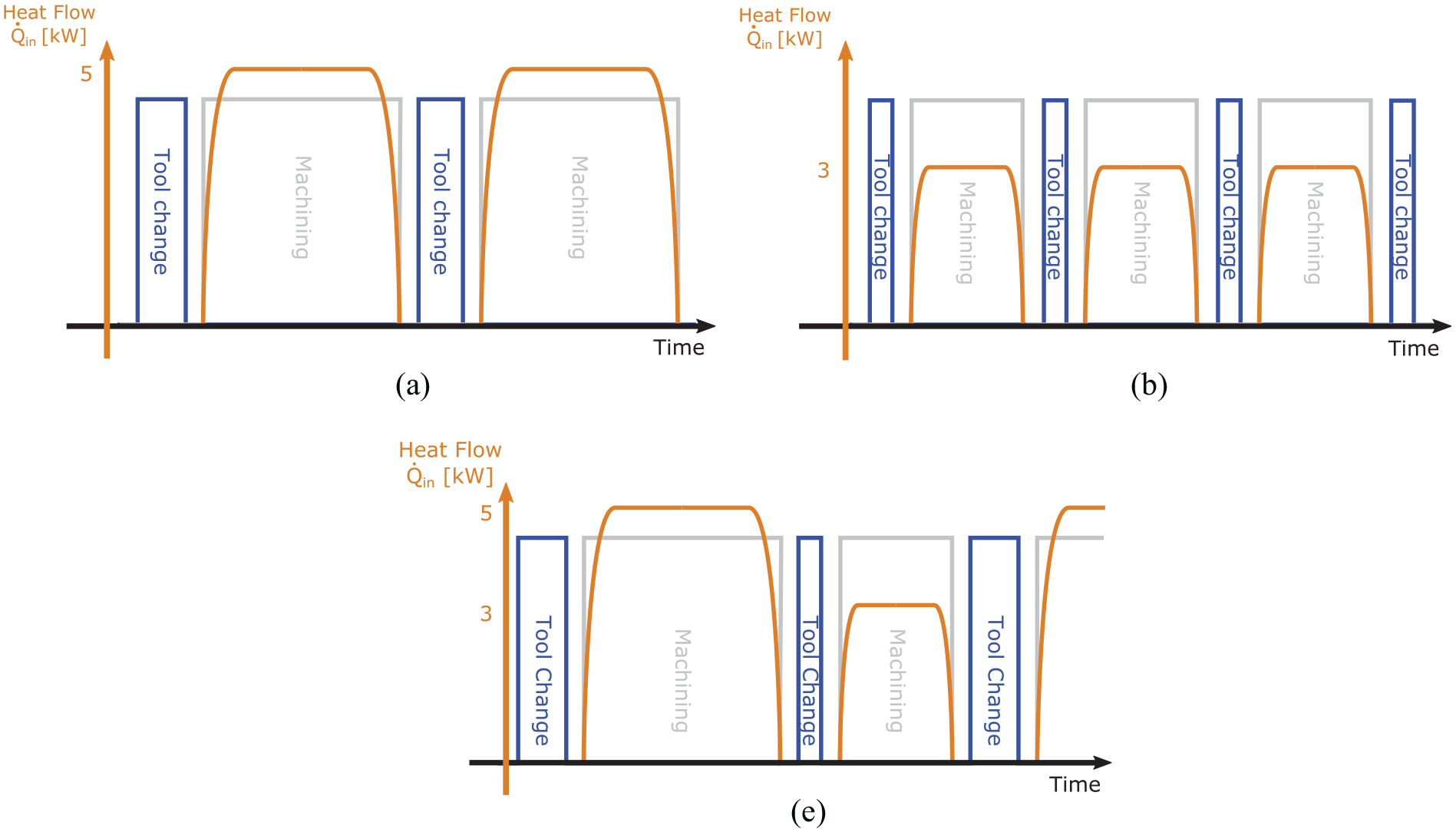
Qualitative structure of the simulated working cycles in terms of machining duty cycle, tool change and heat flow
Figure 7(c) represented a qualitative structure of non-stationary cycles. Two datasets were created, one including SC1 and SC2, the other including NSC1 and NSC2. The output of the digital twin consisted of 41 physical quantities, theoretically measurable through sensors to be mounted on the machine. A total of 108 simulations for each dataset were generated combining all the
Feature extraction
Three global features (from the whole cycle) were extracted for each signal: mean, Skewness and Kurtosis coefficients (Figure 6(c)). Global features provide a significant reduction of the dimensionality, but in some applications, they are not enough to obtain good results and local ones (from parts of the cycle) should be introduced. The features were then normalised to have null mean and unitary standard deviation. 18 For each fault combination, 20 repetitions were obtained adding random Gaussian noise proportional to signals’ RMS. Resulting datasets consisted of 2160 rows and 123 columns (Figure 6(d)).
Feature selection/machine sensorisation
An innovative aspect presented in this paper regards the use of feature selection to obtain useful tips for machine sensorisation. Although applying dimensionality reduction techniques such as Principal Component Analysis or LDA leads to a smaller space to work on, the entire set of features is used and no sensor selection can be done. The proposed feature selection strategy was divided into two steps (Figure 6(e)). The first was dedicated to sensor selection. The score of each feature with respect to the components was computed separately through the One-Way-ANOVA F-statistic 59 :
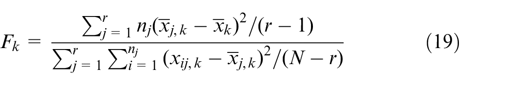
where
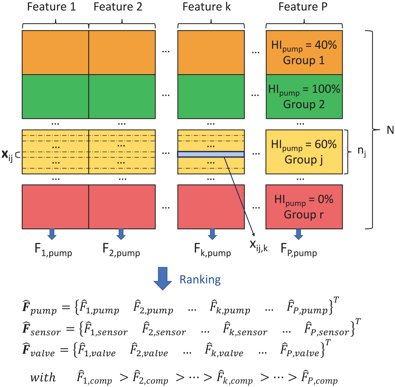
Graphical representation of ANOVA dataset subdivision and scoring.
At the same time, the correlation matrix between features was computed, using Pearson’s correlation coefficient:
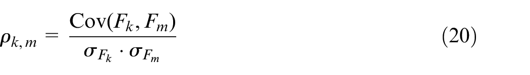
where
The second step consisted of reiterating the computation of the ANOVA scores only on the new features pool and selecting the best features for each component. The novelty of this approach was not only the use of non-correlated features but also the selection of which feature, and consequently which sensor, provided the most valuable information. This step could have consequences on the design of the machine sensorisation. By identifying the best features for the diagnosis purpose, only useful sensors were traced back: seven sensors were used to compute the selected features pool representing 17% of the initial pool. Only the second step of feature selection was needed for the final implementation of the algorithm.
Undersampling/design of experiments
The undersampling technique was applied to reduce the number of experiments for a future validation of the model under faulty conditions. Experimental campaigns can be time-consuming and expensive (e.g. Helwig et al. 11 conducted a total of 2205 tests on a test bench). With regard to the objective of creating an experimental campaign based on the real system, selecting which scenarios to experiment first was needed.
Undersampling, typically applied to imbalanced datasets, 61 was extended to identify the most valuable fault combinations for the classification purpose and consequently for the future experimentation on the real machine (Figure 6(e)). This technique could be applied since a classification model was developed for each component. The dataset was reduced three times (one for each component) and all the shared combinations were stored. In case a particular label is missing after this process, a fault-combination must be reintroduced manually to preserve all the classes of each component. Based on the nearest neighbours rule, NearMiss, 61 the used undersampling technique selected a given number of samples from cluster A which were closest to each instance in cluster B.
As a result, 41 fault combinations were deleted, representing almost 38% of those that were started with. Undersampling was not needed for the final implementation of the algorithm.
Diagnostics
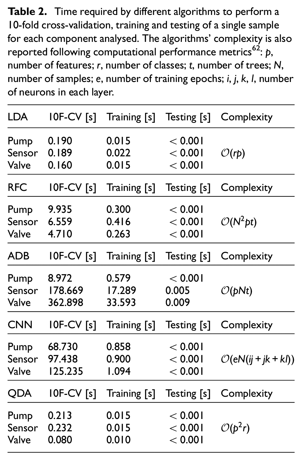
In this work, a tailored diagnosis solution was developed for each component fault (Figure 6(f)). In literature, only one algorithm is selected and tuned for all the components under study. Here, a pool of algorithms was selected: LDA, Random Forest Classifier (RFC), Convolutional Neural Network (CNN), Quadratic Discriminant Analysis (QDA) and AdaBoost Classifier (ADB). The application scenario allowed for supervised learning techniques. In fact, the built datasets consisted of features values for known fault combinations (class labels). Two phases were needed: a training procedure, to update classifier parameters on training data, and a testing procedure to evaluate their performances. In order to compare the algorithms and select the most appropriate one for each component, classification accuracy (or classification rate) was introduced due to its easy interpretation. Performances were investigated both on stationary and non-stationary cycles. For the first ones, a 10-fold cross-validation (CV) was selected, according to the literature. 20 The mean of the accuracy was computed for each classification algorithm. For non-stationary cycles, algorithms were trained upon the stationary dataset and tested on the non-stationary one. In this way, the robustness of the solution was validated on unseen and different working regimes. The time required by the algorithms to perform a 10-fold cross-validation, training and testing was reported in Table 2, together with their complexity.
Time required by different algorithms to perform a 10-fold cross-validation, training and testing of a single sample for each component analysed. The algorithms’ complexity is also reported following computational performance metrics
62
:
The algorithm with the highest final classification rate with respect to a given component was selected as its classifier (in case of a draw, the fastest one was chosen). Diagnosis was then run online at fixed intervals, providing
Prognostics
The proposed prognosis solution can be applied in case run-to-failures or statistical data are available or not. The two associated procedures and algorithm structures were represented in Figure 9.
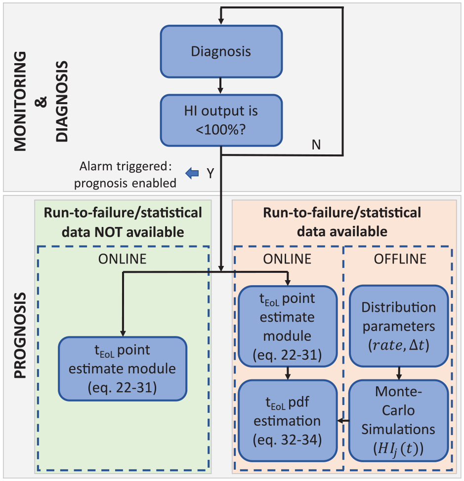
Different strategies for prognosis in the presence, or not, of run-to failure data.
A novelty of this prognosis approach is that it is based on the output of the diagnosis module, that is, a set of
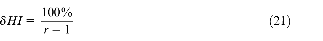
where
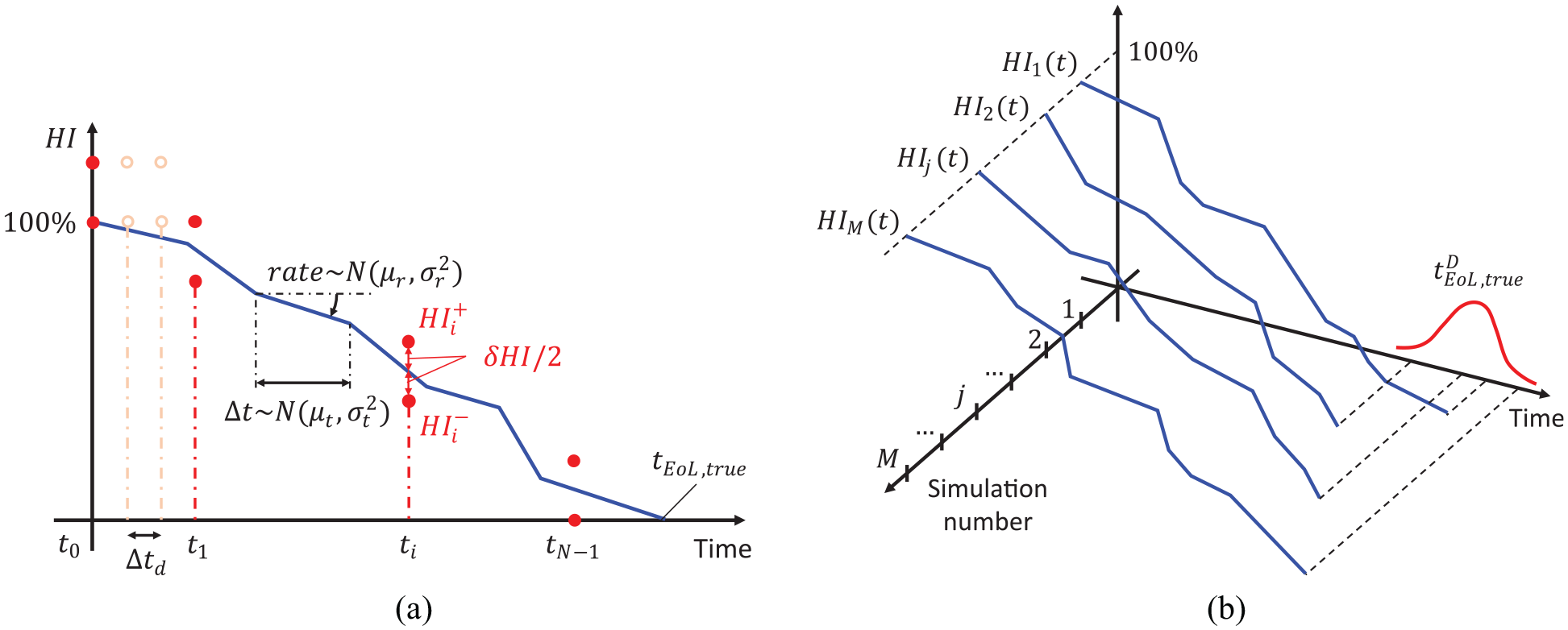
Monte Carlo graphical representation: (a) the actual value of
End of Life (EoL) time point estimate
The procedure in the left branch of Figure 9 could be completely liberated from experimental tests and gives a point estimate of the RUL of a component.
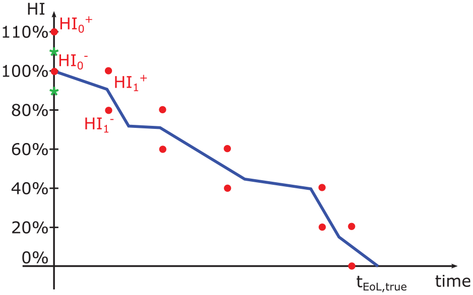
At the end of the degradation process, a monotonic decreasing stair-like

and holds:


with
Except for the starting time instant
1. Compute the line between the last two
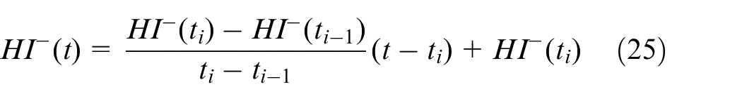
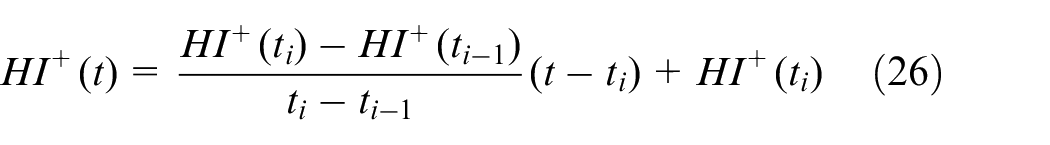
with
2. Compute the EoL estimates imposing:


from which:
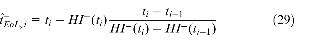
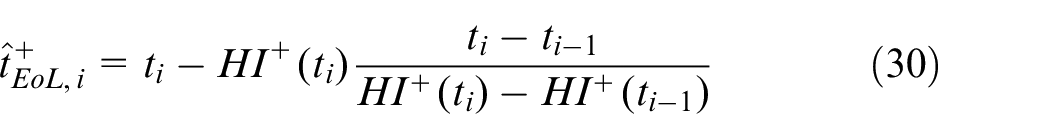
with
3. Compute the unbiased
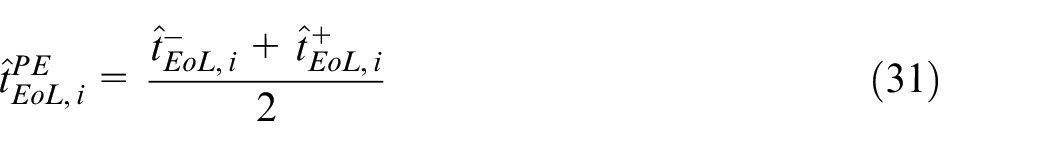
with
The last step is necessary since
Monte Carlo RUL pdf estimation
If run-to-failure tests or statistical data were available, a statistical method for RUL pdf estimation is obtained through the Monte Carlo approach in the right branch of Figure 9. This method is based on the definition of a monotonic decreasing piecewise function which represents the ‘real’ degradation trend of the

with
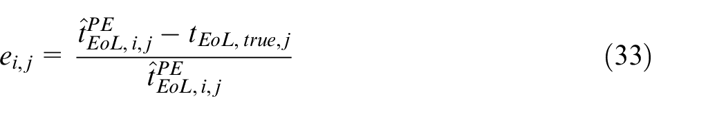
while the error distribution associated with the

The described Monte Carlo approach (up to equation (33)) was used to test the performances of the point estimate module, either in terms of estimation error mean or variance. Here, distributions shown in Figure 10(a) were hypothesised.
Results
Diagnosis
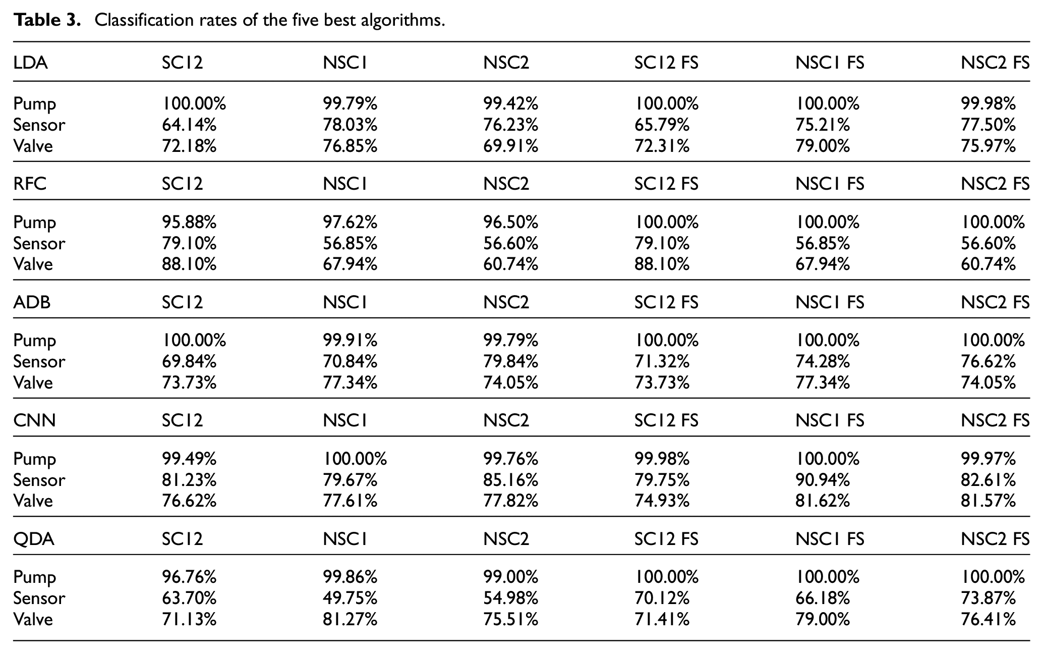
Diagnosis results for all types of working cycle were shown in Table 3. The column labels are explained in the following:
SC12: classification rates for each component based on 10-fold CV for stationary working cycles 1 and 2;
NSC1 and NSC2: classification rates for non-stationary working cycles with training done using stationary working cycles 1 and 2;
suffix FS indicates that the classification rates were obtained with the application of the feature selection.
Classification rates of the five best algorithms.
Prognosis
In order to evaluate the performances of the algorithm, a Monte Carlo based analysis was carried out. In Figure 11, the evolution of the EoL time distributions with respect to the estimation number were shown. Parameters of the distributions shown in Figure 10(a) were hypothesised. As expected, as long as the time of the estimate is approaching the real End-of-Life time of the component, the distributions of the estimated EoL time are getting better, both in terms of expected value and variance. It is worth noting that the first estimate is underestimating the real EoL time. This is due to the fact that, at time instant
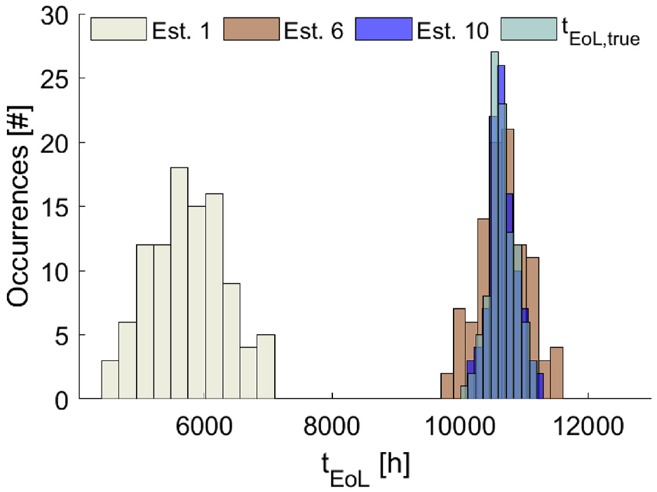
Estimates distribution of
The underestimation problem of the first estimate is due to the different selection criteria of the
By adopting this correction, the lift effect due to the first
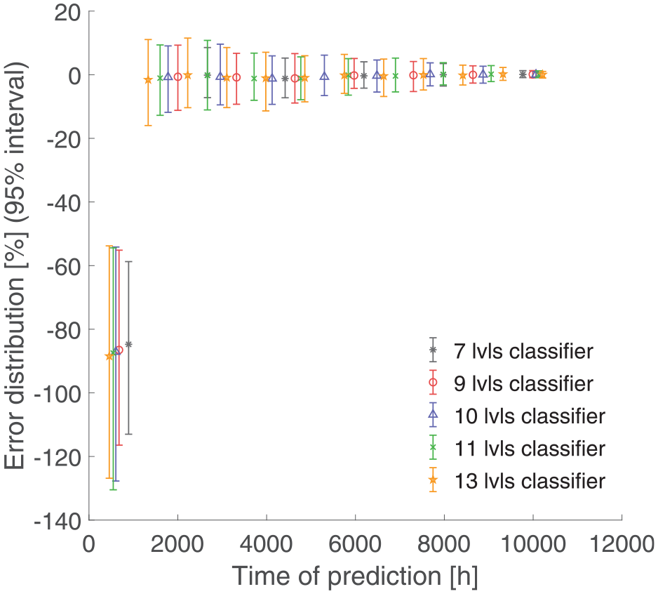
95% error intervals for different classifiers during a component’s life. Five different classifiers are tested with 7, 9, 10, 11, 13 fault states.
In Figure 13, an insignificant difference between the different classifiers is shown: the classifier with the lowest number of fault states shows slightly smaller error intervals, but at the same time, the last estimate is much earlier during the life of the component. In this way, the last estimate of the classifiers with a higher number of fault states are further towards the component EoL allowing a narrower error interval (note that the first estimate is performed earlier but with a bigger error interval). On the other hand, classifiers with a higher number of fault states, require a higher number of tests for training and tend to be more critical in the diagnosis phase. Analysis of performances of the algorithm with respect to other distributions is out of the scope of this paper and will be a matter for future work by the authors.
Conclusions
In this paper, a PHM solution for a machine tool hydraulic unit was presented. Despite the hydraulic unit being one of the most critical part of machine tools,1,3,36 scientific literature was still lacking in this research field. The unavailability of a large amount of faulty data in the life of a machine tool brought about the decision to implement a digital twin of the hydraulic unit. The model was used to generate simulations of the healthy and faulty machine during multiple working cycles:
such a solution was demonstrated to be efficient in addressing the working regime variability, that is, the main limitation for the applicability of prognosis approaches in industry;
the use of a digital twin allowed the support of the sensorisation and the design of experiments for a future validation of the model under fault conditions;
a tailored multi-classifier solution was developed for any component, whereas typical literature solutions are based on a single classifier approach. QDA performed an excellent pump fault diagnosis, while CNN was the best classifier for sensor and valve faults.
the proposed prognosis solution took into account the interaction between different faults, exploiting diagnosis outputs trained on all the fault combinations.
the developed algorithm was able to estimate the RUL probability density function through a Monte Carlo approach.
Proposals for future works include the deployment of the algorithm on a test rig of the system, experimental validation of the digital twin in the presence of faults based on feature selection and undersampling support, and robustness tests on new and unseen working cycles.
Footnotes
Notation
Acknowledgements
The authors would like to thank MANDELLI SISTEMI S.P.A. for their contribution to the project.
Declaration of conflicting interests
The author(s) declared no potential conflicts of interest with respect to the research, authorship, and/or publication of this article.
Funding
The author(s) disclosed receipt of the following financial support for the research, authorship, and/or publication of this article: The project was funded by the Ministero dello Sviluppo Economico (MISE) – Industria Sostenibile FRI–DM 24/07/2015–(Project ref. 55 – B38I17000590008).