Research on the incidence of soft abrasive flow to a wall and the machining characteristics

Abstract

In this study, a calculation model was proposed to predict the motion locus of particles moving to a wall in boundary layers. The velocity of soft abrasive flow and the incident angle of the particles were obtained based on the results calculated by the mixture model and realizable k–ε model. After the model formed, the distributions of the dynamic pressure and the volume fraction of abrasive particles were analyzed and compared to experimental results. After analysis, it was found that the amount of removed material is positively correlated with the incident velocity and the volume fraction of abrasive particles, as well as the dynamic pressure on the surface of the workpiece. In addition, the comparison shows that the numerical simulation method is feasible to predict the flow field and effect of soft abrasive flow. In addition, it was found that the simulation results are consistent with the flow field distribution and machining effect. Therefore, this model can be used in design of constrained modules.

Introduction

Finishing is an important process of mold making, which improves the surface quality of the mold. According to the different working conditions and finishing requirements, some new finishing methods are taking the place of traditional methods, such as gasbag polishing and electrochemical polishing. ¹ What’s more, products are getting miniaturized so that micromanufacturing processes are expanding in their length and breadth.^2,3 As for those complex structures on the mold surface, such as tiny grooves, holes, and narrow flow fields, traditional finishing methods do not work well. For structural surface finishing, fluidic finishing methods are proposed. Shiming Ji from Zhejiang University of Technology proposed a new method called the soft abrasive flow (SAF) finishing.^4–6 Based on this, Li et al. ⁷ improved this method by adding ultrasonic field. Also, Zhang et al. ⁸ studied the process of abrasive flow machining for the titanium alloy artificial joint surface and provided the basis for optimizing the structure of the flow channel. SAF, a weak-viscous fluid with good liquidity, can form turbulence in the constrained channel, which is the gap between the finishing surface and the constrained module. The abrasive particles in the turbulence impact the surface to cut it so that molds are finished without tools. A constrained module is proposed based on the SAF finishing method. Constrained modules in different shapes can form different flow channels to control the flow field so that different finishing effects can be reached. Because of the constrained module, the turbulence in the finishing area can be strengthened so that more particles can go through the boundary layer and impact the surface. Meanwhile, by changing the incident angle and velocity of particles, the surface can be finished in different stages and areas.

Due to the complexity of the flow field, the process of designing constrained modules experimentally is expensive and inefficient. Therefore, CFD (Computational Fluid Dynamics) software is essential in the beginning of the design. However, CFD software has a limitation. In the simulation of the two-phase flow field, the models of the solid phase are always considered a pseudofluid model, ⁹ in which case the default velocity of the solid phase in the boundary layer is 0, and this is not consistent with the actual condition of the flow field. When the abrasive particle enters the boundary layer of fluid, it will maintain its original motion due to inertia, ¹⁰ and scratches are created by these particles. Due to the limitation of the CFD software, especially the imprecise simulation of the high-volume-fraction solid phase, studies on SAF finishing methods are constrained. Therefore, it is necessary to find a simple method to calculate the incident angle and the velocity of solid particles based on the simulation of the flow field in a constrained channel. With the new method, theoretical calculations and experimental data can be compared to provide references for processing parameters of SAF, such as the velocity of SAF, volume fraction of solid phase, and diameter of particles.

Wang found that the velocity of the nanoparticles was significantly different with that of water and the transfer of momentum between the two phases is obvious, which make the boundary layer thinner. ¹¹ Sun studied the solid particle behavior in boundary layers via particle imaging velocimetry (PIV). It is showed that the turbulence of large particles is larger than that of small particle, and the particle flow turbulence is greater than normal turbulence.^12,13 Li et al. ¹⁴ found that the particle streamwise fluctuating velocity exceeds the fluid streamwise fluctuating velocity across the entire boundary layer.

A calculation model for particles moving into the boundary layer is proposed in this study so that the incident angle of the solid substances and the velocity of SAF can be calculated by the model. Simultaneously, due to the complexity of the design for the structure of constrained modules, the tests were performed with the simplest constrained channel and then compared the results with the simulation data to verify the reliability of the simulation data and evaluate the processing effect. The corresponding relationship between the constrained module design parameters, flow field data, grinding particle incidence state, and processing effect can provide references for other designs.

Simulation and data processing

Simulation model and boundary condition

To facilitate the measurement of the roughness of the workpiece surface and microscopic observation of the forms on the surface, some removable metal strips were used as the bottom of the flow channel and constrained modules were used at the top to form a channel. The constrained modules can be designed in a variety of structures to control the movement of the abrasive flow to influence the processing. In this study, the three-dimensional (3D) model of the constrained flow channel is shown in Figure 1.

Figure 1.

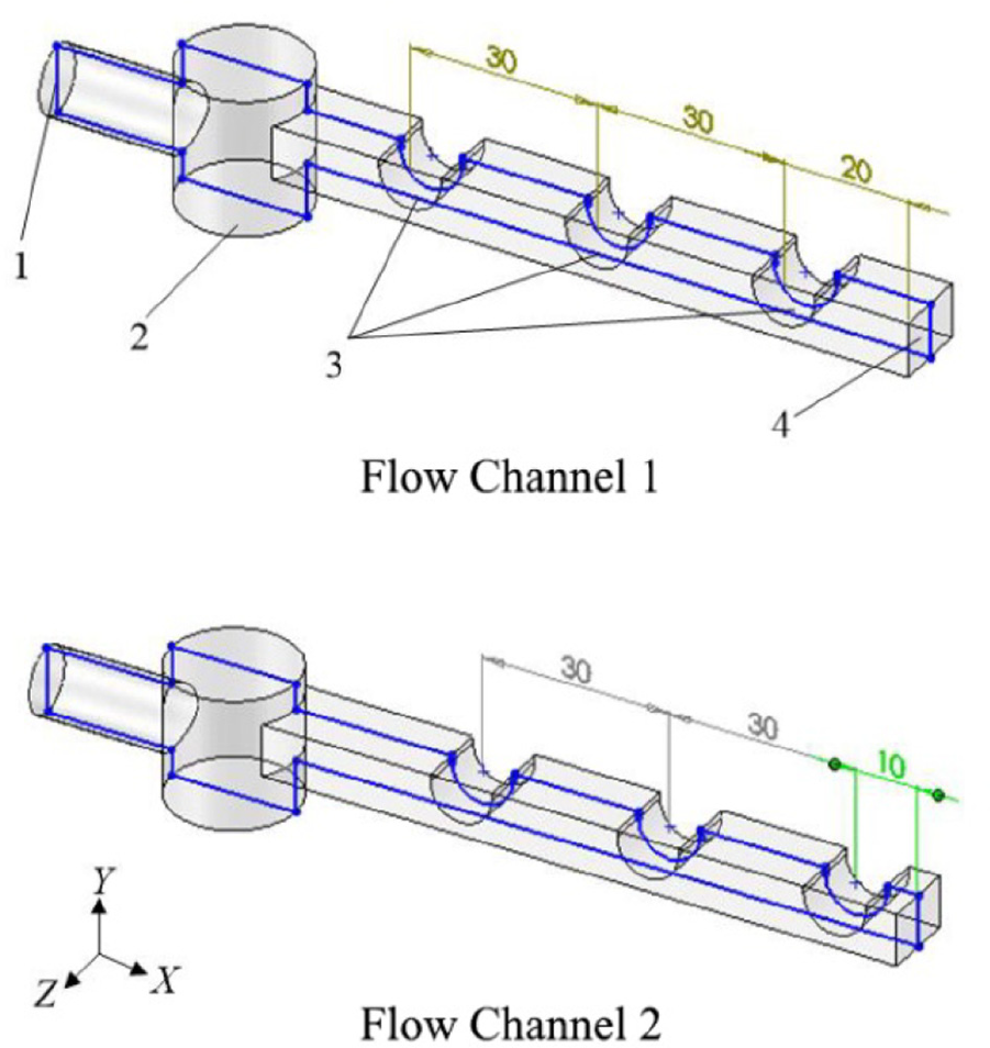
3D models of two flow channels.

The abrasive flow is in the x direction. First, the flow enters the cylindrical turbulence generator. Then, it enters the constrained flow channel with three protrusions and finally flows out from the outlet. Because the size of the flow channel in the z direction is consistent, the middle section of the flow channel in the z direction is taken for further calculation.

Because the realizable k–ε turbulent model can describe the boundary layer accurately, ¹⁵ this turbulent model is used for simulating the SAF flow field. The boundary condition of the simulation is that the inlet condition is the velocity inlet, and the outlet condition is the outflow. Because the flow of the submersible pump is 10 m³/h and the diameter of the outlet is 10 mm, the velocity at the inlet is 25 m/s. The solid phase is SiC, and the liquid phase is water. The volume fraction of the solid phase is 30%, and the diameter of solid phase is 10 μm.

The analysis of simulation results

The flow field in the constrained channel shows a certain rule under the action of the constrained module, as shown in Figures 2 and 3.

Figure 2.

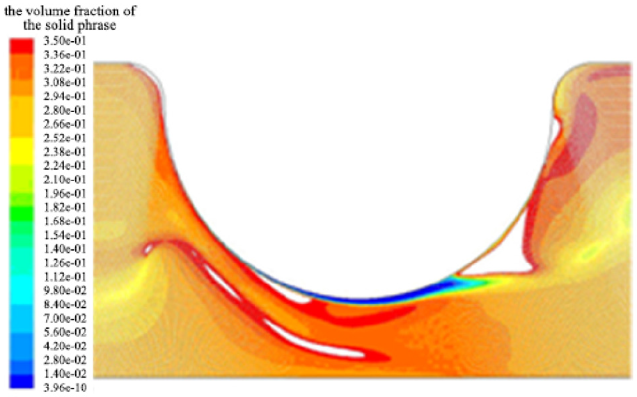
The profile of the volume fraction distribution of the solid phase after the first convex.

Figure 3.

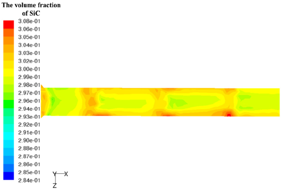
The volume fraction of SiC on the flow passage bottom.

As shown in Figure 2, to more clearly demonstrate the difference in the distribution of the solid phase volume fraction in each region, the maximum value of the cloud map is set as 35%, and the value of the blank area is greater than 35%. Because the density of the solid particles is larger than that of the liquid, the original motion of these particles is stronger than that of the liquid after flowing through the constrained protrusion due to inertia; thus, the volume fraction of solid particles is extremely low in some regions. As shown in Figure 3, the volume fraction of SiC on the bottom of the flow channel increased at these three protrusions, and it was concluded that in these three areas, more particles will impact the surface to finish it.

Figure 4 shows the dynamic pressure of the SAF field on the bottom of the flow channel. Under the influence of the protrusions, the fluid will impact the surface at a certain angle, so the dynamic pressure at these three protrusions is higher than at other areas. Meanwhile, circumfluence appeared when the fluid flowed through the first protrusion due to negative pressure. In this case, not only the normal-direction vortex appeared in the x-O-y plane but the spanwise vortex appeared in the x-O-z plane as well. ¹⁶ As shown in Figure 5, the streamline is analyzed by taking a section 6 mm away from the machined surface.

Figure 4.

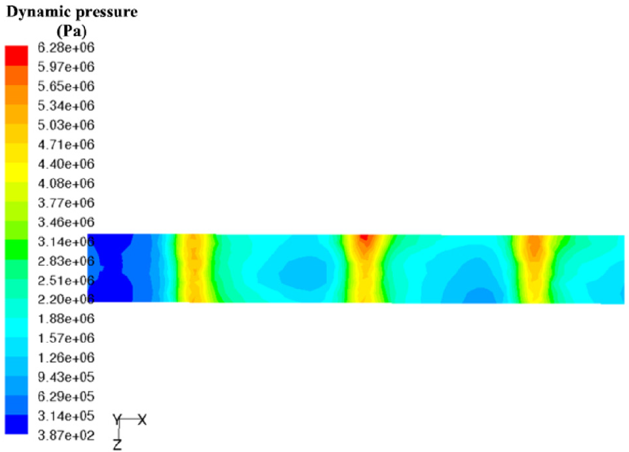
The bottom surface pressure of runner 1.

Figure 5.

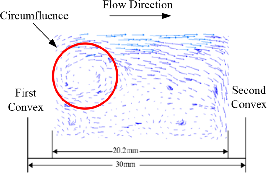
The planar streamline chart of the runner 1 at a 6-mm distance from the bottom.

In the simulation, the default velocity of the boundary layer is 0, so the motion characteristics of the SAF in the boundary layer can be derived only by analyzing the characteristics in the areas near the wall. In Figure 5, the circumfluence appeared because of the protrusions of the constrained module. After the first protrusion, the cross-sectional area of flow channel became larger and the particles affected by the vortex flowed back to the center of the flow channel. This result is demonstrated by the distribution of the volume fraction of SiC on the bottom of the flow channel, which is shown in Figure 3.

Processing of simulation data

To improve the practicality of the simulation, a calculation model for the velocity and the incident angle of the particles is proposed. The motion track of the particles near the wall after entering the boundary layer is calculated on the basis of the fluent calculation data, and the velocity and the incident angle of the particles hitting the wall are estimated.

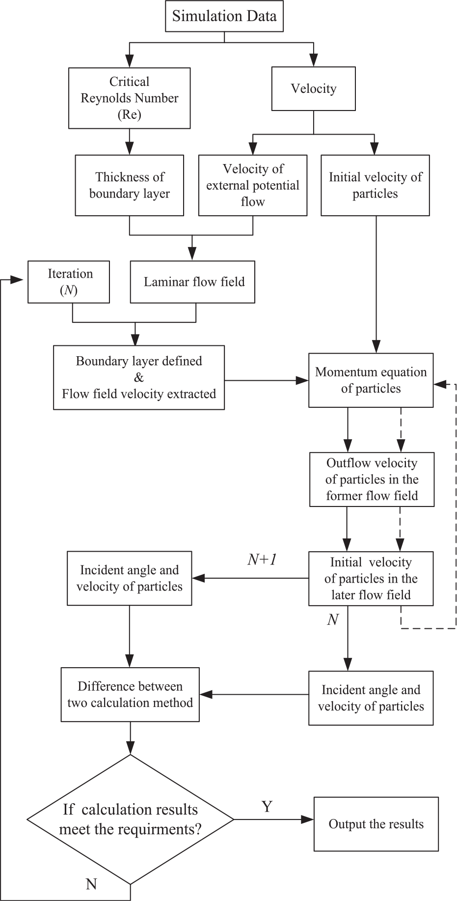
The calculation procedure is shown in Figure 6. First, the simulation data can be obtained from the results of the numerical simulations. In the SAF, the density of the solid phase is much greater than that of the liquid phase. When the velocity of the SAF has a sudden change, the motion and velocity of the solid phase will remain due to the inertia. Therefore, the velocity of particles in the boundary layer can be considered the same as before impact. Then, the Reynolds number (Re) of the SAF was obtained by calculation, and the results are contrasted with the critical Reynolds number to derive the thickness of the viscous sublayer of the surface. Based on the thickness of viscous sublayer, the velocity distribution of the laminar flow field can be obtained. After, we divide the laminar flow field to solve the momentum equation of the particles in the viscous sublayer. When the parameters of the next calculating area are analyzed, the last calculating results can be substituted into the equation of the new area. Finally, the motion parameters of the abrasive particles hitting the wall surface are determined. To ensure the accuracy, the threshold value can be set so that the calculation result caused by the precision of the dividing boundary layer is within the required range.

Figure 6.

The diagram of the model structure of the incident trajectory of the particles.

Divide the boundary layer

Due to the liquid viscidity of the boundary layer of the turbulent flow field, the molecular viscous force has a greater influence than the inertia, and under the influence of the viscous force, the fluctuating velocity of the fluid is gradually weakened. The boundary layer can be divided into three parts: the viscous sublayer, the transition layer, and the turbosphere. In the viscous sublayer, the effect of the viscous force is greater than that of the inertia so the flow is laminar; meanwhile, due to the interaction between the surfaces of the flow channel, the turbulent intermittency between the potential flow and the boundary layer does not appear, so the transition layer of the SAF in the boundary layer does not exist either. ¹⁷

In the CFD simulation software, the enhanced wall treatment (EWT) method is used to calculate the characteristics of the walls near the complex flows. In this method, the turbulent Reynolds number (Re _y ) based on the wall distance is used to determine whether the viscidity or the turbulence is dominant in this flow field. The calculation of Re is shown as equation (1)

$${\mathrm{Re}}_y=\frac{\rho y\sqrt{k}}{\mu }$$

(1)

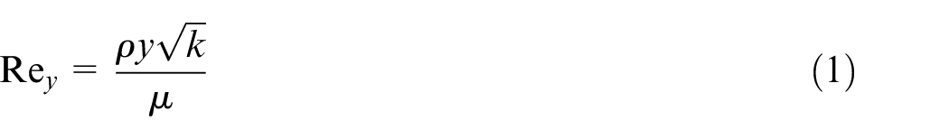
where ρ is the density of fluid; y is the distance to the wall; k is the turbulence energy; and μ is the turbulent viscosity.

When the Re _y  < 200, the flow field is considered as a viscous area. In this field, the molecular force is dominant, and the inertia is the subordinate. In this case, the flow in this field is laminar.

In this calculation method, the Re of the fluid in the areas near the wall is extracted from the simulated data. In this way, the area of which the Re is 200 would be confirmed, and the value of the distance from this area to the surface is the estimated value of thickness of the boundary layer. With this method, the thicknesses of the viscous sublayer of these two constrained flow channels in Figure 1 are obtained.

As shown in Figure 7, the maximum of the thickness of the boundary layer appeared at the inlets of these two flow channels and the minimums appeared at each protrusion of constrained flow channel. In the inlet, the cross-sectional area of the flow channel decreased suddenly. The SAF in this area turned into turbulence gradually. Near the protrusions of the constrained flow channel, the velocity of the SAF increased due to the decrease of the cross-sectional area, which decreased the thickness of the boundary layer. After the SAF went through the protrusions, the cross-sectional area of flow channel became larger. Pulsations appeared under the effect of negative pressure and the thickness of the boundary layer increased. Compared with two flow channels in Figure 1, the rules of the changes of these two flow fields are similar. However, the different positions of the protrusions led to decreases of the thicknesses of the boundary layers in different areas.

Figure 7.

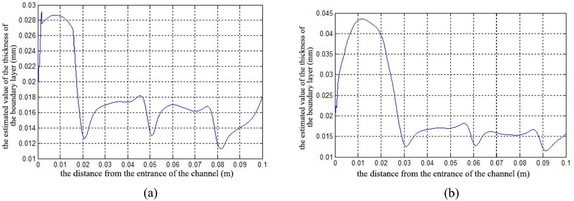
Two types of boundary layer thickness values of the constrained flow channel bottom surface: (a) flow channel 1 and (b) flow channel 2.

Velocity distribution in the boundary layer

To facilitate calculation, the flow in the boundary layer can be assumed as laminar flow. Based on the velocity function from K. Pohlhausen, ¹⁸ the distribution of the velocity in the boundary layer can be described as equation (2)

$$\frac{u}{U}=f\left(\eta \right)=a\eta +b{\eta }^2+c{\eta }^3+d{\eta }^4$$

(2)

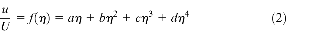
where $\eta =y/\delta ,0\le \eta \le 1$ ; u is the velocity in the boundary layer; U is the velocity of the potential flow out of the boundary layer; y is the distance of the boundary layer to the surface; and δ is the thickness of the boundary layer.

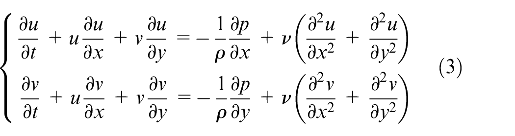
By ignoring the body force, the two-dimensional (2D) Navier–Stokes equation can be simplified as equation (3)

$$\{\begin{array}{c}\multicolumn{1}{c}{\frac{\partial u}{\partial t}+u\frac{\partial u}{\partial x}+v\frac{\partial u}{\partial y}=-\frac{1}{\rho }\frac{\partial p}{\partial x}+\nu (\frac{{\partial }^{2}u}{\partial x^2}+\frac{{\partial }^{2}u}{\partial y^2})}\\ \multicolumn{1}{c}{\frac{\partial v}{\partial t}+u\frac{\partial v}{\partial x}+v\frac{\partial v}{\partial y}=-\frac{1}{\rho }\frac{\partial p}{\partial y}+\nu (\frac{{\partial }^{2}v}{\partial x^2}+\frac{{\partial }^{2}v}{\partial y^2})}\end{array}$$

(3)

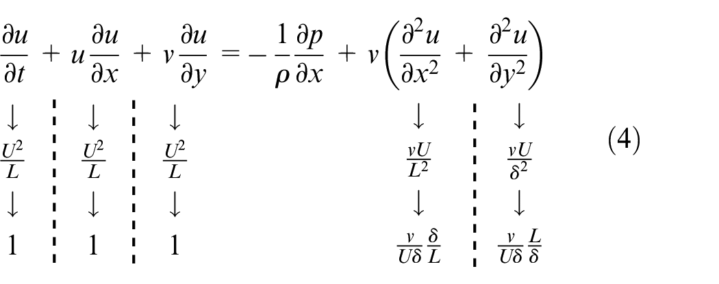
With scale analysis, ¹⁹ $x~L$ , $y~\delta$ , $t~L/U$ , $v~U\delta /L$ , and the 2D Navier–Stokes equation can be scale analyzed as equations (4) and (5)

$$\begin{array}{ccccccccc}\frac{\partial u}{\partial t}\hfill & +\hfill & u\frac{\partial u}{\partial x}\hfill & +\hfill & v\frac{\partial u}{\partial y}=-\hfill & \frac{1}{\rho }\frac{\partial p}{\partial x}+v(\hfill & \frac{{\partial }^{2}u}{\partial x^2}\hfill & +\hfill & \frac{{\partial }^{2}u}{\partial y^2})\hfill \\ \downarrow \hfill & \hfill & \downarrow \hfill & \hfill & \downarrow \hfill & \hfill & \downarrow \hfill & \hfill & \downarrow \hfill \\ \multicolumn{1}{c}{\frac{U^2}{L}}& \hfill & \frac{U^2}{L}\hfill & \hfill & \frac{U^2}{L}\hfill & \hfill & \multicolumn{1}{c}{\frac{\mathrm{vU}}{L^2}}& \hfill & \frac{\mathrm{vU}}{{\delta }^2}\hfill \\ \multicolumn{1}{c}{\downarrow }& \hfill & \downarrow \hfill & \hfill & \downarrow \hfill & \hfill & \downarrow \hfill & \hfill & \downarrow \hfill \\ \multicolumn{1}{c}{1}& \hfill & 1\hfill & \hfill & 1\hfill & \hfill & \multicolumn{1}{c}{\frac{v}{U\delta }\frac{\delta }{L}}& \hfill & \frac{v}{U\delta }\frac{L}{\delta }\hfill \end{array}$$

(4)

$$\begin{array}{ccccccccc}\frac{\partial v}{\partial t}\hfill & +\hfill & u\frac{\partial v}{\partial x}\hfill & +\hfill & v\frac{\partial v}{\partial y}=\hfill & -\frac{1}{\rho }\frac{\partial p}{\partial x}+v(\hfill & \frac{{\partial }^{2}v}{\partial x^2}\hfill & +\hfill & \frac{{\partial }^{2}v}{\partial y^2})\hfill \\ \downarrow \hfill & \hfill & \downarrow \hfill & \hfill & \downarrow \hfill & \hfill & \downarrow \hfill & \hfill & \downarrow \hfill \\ \multicolumn{1}{c}{\frac{U^2}{L}\frac{\delta }{L}}& \hfill & \frac{U^2}{L}\frac{\delta }{L}\hfill & \hfill & \frac{U^2}{L}\frac{\delta }{L}\hfill & \hfill & \multicolumn{1}{c}{\frac{\mathrm{vU}}{L^2}\frac{\delta }{L}}& \hfill & \frac{\mathrm{vU}}{{\delta }^2}\frac{\delta }{L}\hfill \\ \multicolumn{1}{c}{\downarrow }& \hfill & \downarrow \hfill & \hfill & \downarrow \hfill & \hfill & \downarrow \hfill & \hfill & \downarrow \hfill \\ \multicolumn{1}{c}{\frac{\delta }{L}}& \hfill & \frac{\delta }{L}\hfill & \hfill & \frac{\delta }{L}\hfill & \hfill & \multicolumn{1}{c}{\frac{v}{U\delta }{\left(\frac{\delta }{L}\right)}^2}& \hfill & \frac{v}{U\delta }\hfill \end{array}$$

(5)

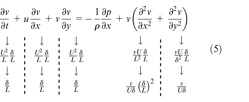
The boundary layer Prandtl equation of steady flow can be described as equation (6) ²⁰

$$\{\begin{array}{c}\frac{\partial u}{\partial x}+\frac{\partial v}{\partial y}=0\hfill \\ \multicolumn{1}{c}{u\frac{\partial u}{\partial x}+v\frac{\partial u}{\partial y}=-\frac{1}{\rho }\frac{\partial p}{\partial x}+\nu \frac{{\partial }^{2}u}{\partial y^2}}\end{array}$$

(6)

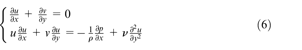
By equation (6)—equation (2)—derived boundary conditions, the reason why the speed function is set as four functions is that there are only four boundary conditions as follows

When $y=0,u=v=0$

$$\nu \frac{{\partial }^{2}u}{\partial y^2}=\frac{1}{\rho }\frac{\mathrm{dp}}{\mathrm{dx}}=-\mathrm{KU}\frac{\mathrm{dU}}{\mathrm{dx}}$$

(7)

When $y=\delta ,u=U,v=0$

$$\frac{\partial u}{\partial y}=0,\frac{{\partial }^{2}u}{\partial y^2}=0$$

(8)

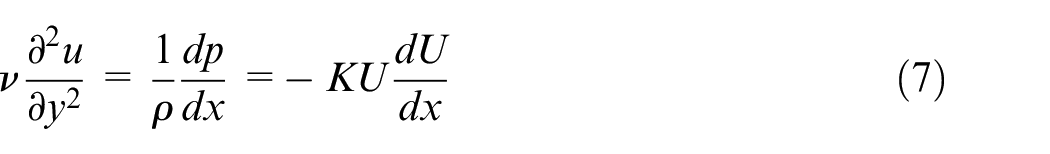
A solid perturbation coefficient K is added. ²¹ The coupling force that is exerted on fluid by solid particles is added to boundary conditions. And its effect on calculating the thickness of the boundary layer is indicated in the form of the ratio of the coupling force to the resultant force exerted on the fluid

$$K=\frac{F_d}{{\mathrm{PX}}_{\mathrm{cf}}}$$

(9)

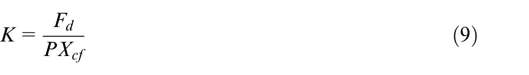
In formula (9), F_d is the force of the particle effect on fluid; χ_cf is the solid phase concentration coefficient; p is the fluid pressure, and v is the kinematic viscosity.

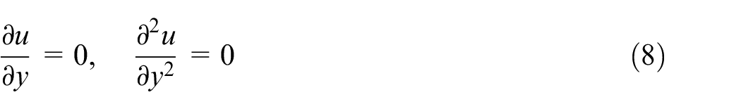
Formula (8) is concluded from the hypothesis of a physical phenomenon. At the junction of the boundary layer, the speed inside the boundary layer is equal to the outside, the speed change rates are equal, and the shear stress is equal.

After the operation, the result can be obtained

$$\{\begin{array}{c}a+b+c+d=1\hfill \\ \multicolumn{1}{c}{b+3c+6d=0}\\ \multicolumn{1}{c}{a+2b+3c+4d=0}\\ \multicolumn{1}{c}{b=-\frac{1}{2}K\frac{{\delta }^2}{\nu }\frac{\mathrm{dU}}{\mathrm{dx}}}\end{array}$$

(10)

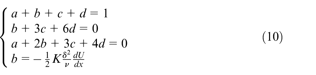
By calculating formula (10), the values of a, b, c, and d can be obtained, and using formula (2) can calculate the flow velocity distribution of the bottom layer processing of each point on the surface of the clay.

The analysis of the motion of the particles inside the boundary layer

From the analysis of the velocity of the flow field, the distribution of the velocity of the second phase fluid is similar to that of the first phase fluid. They both had a good velocity gradient into the boundary layer until the velocity turned to zero. To calculate the speed and the incident angle of particles impacting the wall, the velocity of the second phase particles before entering the boundary layer is taken as the initial velocity before the incident boundary layer.

The motion of solid particles is solved by the differential equation of particle forces under the integral Lagrangian coordinate system. ²² Particles in the flow field are affected by the constant resistance, the force attached with acceleration, and the uneven force from the fluid without considering the sum of the external force, such as buoyancy. The force attached with acceleration includes the additional inertia force and the Basset force. The uneven force includes pressure gradient force and speed gradient force. The speed gradient force contains the force of Magnus and the force of Saffman^23,24

$$\begin{array}{c}\multicolumn{1}{c}{m_p\frac{d{u}_p}{\mathrm{dt}}=m_{p}g+F_D+F_{\mathrm{VM}}+F_B}\\ \multicolumn{1}{c}{+F_P+F_{\mathrm{ML}}+F_{\mathrm{SL}}+F_x}\end{array}$$

(11)

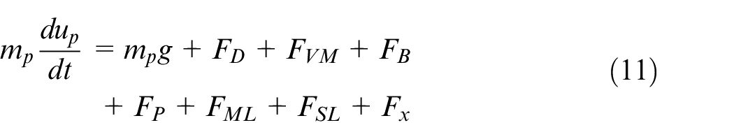
Ignoring the rotation motion of the particles, the force analysis includes the gravity, the constant resistance, the pressure gradient force, and the Saffman force. Meanwhile, because the size of the particles is too small, the pressure gradient force and the Saffman force can be ignored. Therefore, the constant resistance was only considered for the analysis of the trajectories of the particles.

The constant resistance is given in the form of the flow resistance

$$F_d=\frac{3{\mu }_f}{{\rho }_{\mathrm{pp}}{d}_p^2}\frac{C_d{\mathrm{Re}}_p}{4}(u_f-u_p)$$

(12)

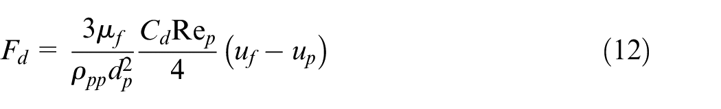
Among them, F_d is the constant resistance; μ_f is the dynamic viscosity coefficient; u_p is the particle speed; ρ_pp is the particle’s density of the material; d_p is the particle diameter; C_p is the resistance coefficient; Re _p is the particle Reynolds number; and C_d is the resistance coefficient

$${\mathrm{Re}}_p=|u_f-u_p|\frac{d_p}{{\nu }_f}$$

(13)

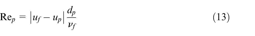
where ν_f is the kinematic viscosity coefficient

$$C_d=\left\{\begin{array}{c}\mathrm{when}\mathrm{Re}\le 0.2\hfill \\ \multicolumn{1}{c}{\frac{24}{{\mathrm{Re}}_p}}\\ \multicolumn{1}{c}{\mathrm{when}0.2<\mathrm{Re}<800}\\ \multicolumn{1}{c}{\frac{24}{{\mathrm{Re}}_p}(1+0.15{{\mathrm{Re}}_p}^{0.687})}\end{array}\right\}$$

(14)

The momentum differential equation of a single abrasive particle in the boundary layer is as follows

$$\begin{array}{cc}\multicolumn{1}{c}{\frac{1}{6}\pi d_p^3{\rho }_{\mathrm{pp}}\frac{d{u}_{\mathrm{pi}}}{\mathrm{dt}}=}& 3\pi {\mu }_f{d}_p(u_{\mathrm{fi}}-u_{\mathrm{pi}})\hfill \\ +\frac{1}{6}\pi d_p^3{\rho }_{\mathrm{pp}}{g}_i\hfill \end{array}$$

(15)

Formula (15) is the expression of tensor. In this formula, g is the gravity acceleration; and the subscript i is the direction of x or y.

We can obtain the velocity of the particles in the boundary layer by combining formulas (15) and (2). The velocity before incidence, the velocity after incidence, and the angle of incidence are obtained by processing the data via MATLAB. As shown in Figure 8, under the action of the constrained module, the velocity in x direction increased after the flow went through each protrusion. In addition, the second and third protrusions affected the velocity in y direction are less than the first.

Figure 8.

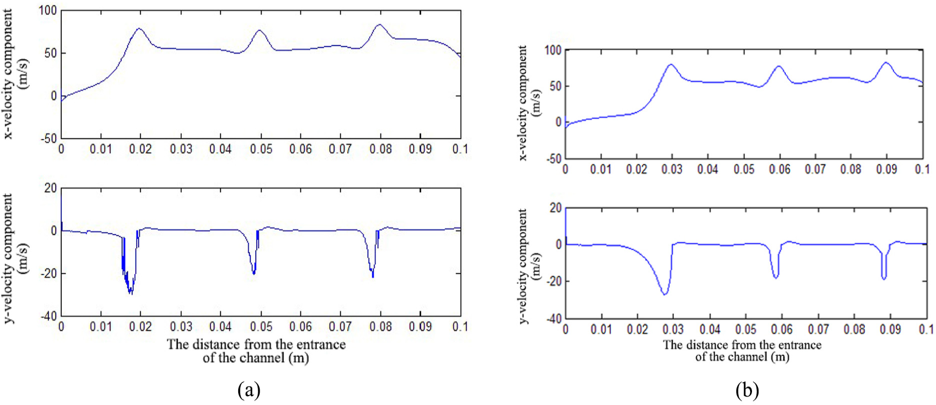
Velocity distribution of the particles at the bottoms of the two channels before the incidence: (a) flow channel 1 and (b) flow channel 2.

As shown in Figure 9, the velocity and the incidence angle of the abrasive particles hitting the wall surface after going into the boundary layer were obtained via iterative computations. To facilitate and describe the state of motion of the incident particles, we took the flow direction as the positive direction of the x-axis and the normal direction of the surface as the positive direction of the y-axis. The discontinuous points illustrate that the particles did not have enough kinetic energy to penetrate the boundary layer. In MATLAB, the discontinuous points were regarded as NaN (not a number).

Figure 9.

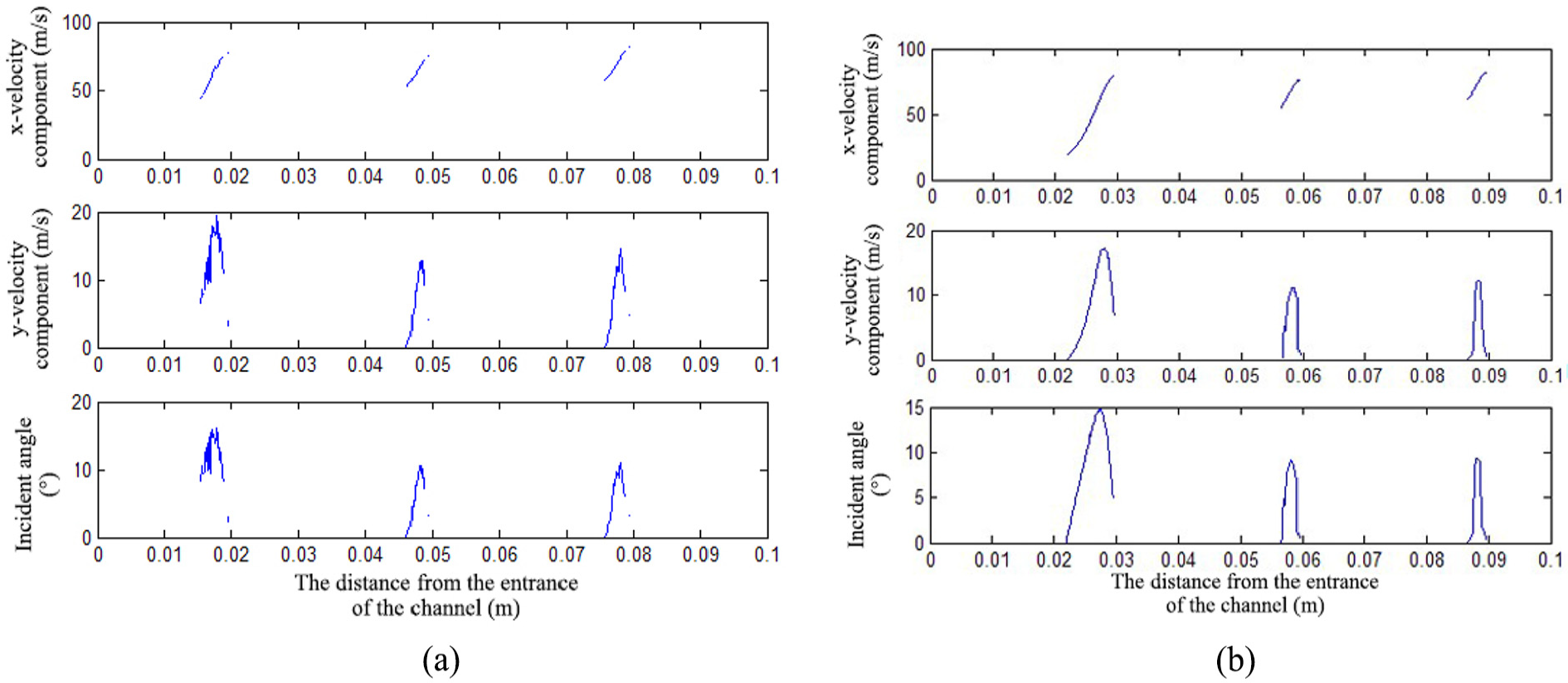
Velocity distribution of the particles of the bottoms of the two channels after the incidence: (a) flow channel 1 and (b) flow channel 2.

This calculation model can solve the problem that the default velocity of the particles hitting a wall is zero in CFD software and is feasible to predict the motions of the particles.

Experiment and the results

Building the experimental platform

According to the simulation model, the same constrained flow channel is established for the abrasive flow. The water tank is filled with solid–liquid abrasive flow. Then, the agitator is turned on in the water tank before processing to suspend the abrasive particles in the water tank and sent the fluid into the flow channel using a submersible pump. Finally, the fluid flowed back to the water tank from the outlet of the flow channel. The constrained flow channel is composed of constrained modules, fixtures, and sealing gaskets. The submersible pump lift is 15 m, and its flow is 10 m³/h. The abrasive flow is composed of water and SiC particles, whose size is 10 μm. And 45 steel is chosen.

The result of experiment

First, we took the pictures of the surfaces of two test workpieces in channels 1 and 2 using a microphotographic camera and then measured their roughness to compare and evaluate the processing effect.

Areas A, B, C, D, F, and E in Figure 10, which corresponded to the protrusions, were brighter than other areas and became brighter along the positive direction of the x-axis. In areas B, C, E, and F, deep grooves appeared along both sides of the flow channel, which was consistent with the image of SiC particle volume fraction distribution (Figure 3) in the simulation data. After comparing areas A, D, B, and E to areas C and F, it was found that the removal amount increased when the constrained protrusions shifted in the x direction.

Figure 10.

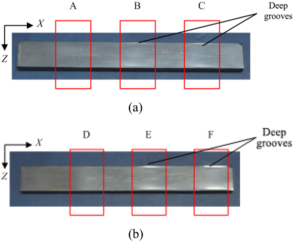
Tested workpieces: (a) the machining workpiece of flow channel 1 and (b) the machining workpiece of flow channel 2.

From the distribution of the velocity field, it was found that after the fluid passed a protrusion, the cross-sectional area inside the flow channel increased and produced a negative pressure zone so that the fluid is subjected to entrainment and produces eddy currents. The entrainment in the middle of the flow channel was stronger than that in the area of the walls because there was no boundary layer in the middle area of the flow channel. Before entering the second constrained projection structure, as the entrainment function between the first and the second protrusions in the direction of z-axis is uneven, the fluid in the middle of the flow channel spreads to both sides of the flow channel under the effect of the entrainment. Therefore, the processing of both sides of the channel was more obvious after the abrasive flow passes through the second protrusion. Simultaneously, the abrasive particles cannot enter into the corners of the flow channel for processing due to the boundary layer, so a protrusion of an unprocessed area appeared on the boundary, which formed a deep groove.

To observe the difference of machining efficiency among different areas more clearly, another workpiece was tested in which three different parts were painted in three different colors. As shown in Figure 11, after a 2-h processing, the middle part of the flow channel was abraded more heavily in area G. In area H, the effect of the processing on both sides of the channel was more obvious. Meanwhile, at the bottom of the channel, the removal amount was smallest in area I. The experimental results were consistent with the cloud map of dynamic pressure distribution in the flow passage (Figure 4). The processing efficiency in the high dynamic pressure area was more efficient.

Figure 11.

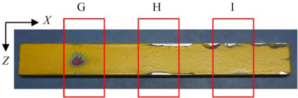
The surface of the workpiece in the process of spray paint testing.

To observe the machining effect, the surface of the workpiece was photographed with microphotographic equipment, and the magnification was 500 times. By comparing Figure 12(a) with Figure 12(b), it was found that the original processing traces were eliminated. By comparing Figure 12(c) with Figure 12(d), the processing effect at the protrusions was more obvious than the corresponding areas where there were no protrusions. The 3D simulation diagram (Figure 12(e) and (f)) showed that the processing texture became disordered.

Figure 12.

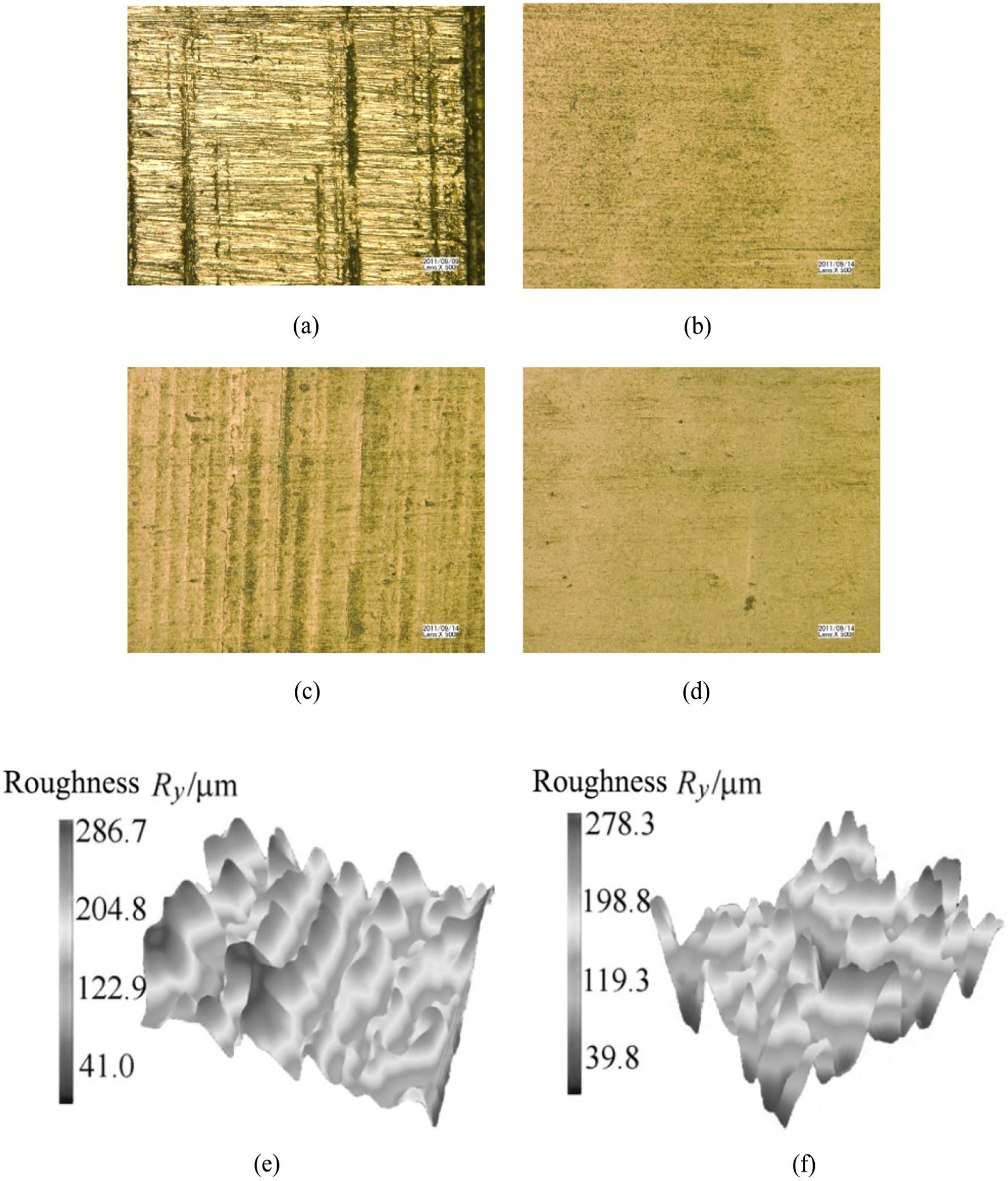
Magnification 500 times surface topography photos and 3D simulation: (a) unprocessed micrograph 500×, (b) after processing micrograph 500×, (c) nonconstrained projection correspondence region 500×, (d) constrained projection correspondence region 500×, (e) 3D simulation before machining, and (f) 3D simulation after machining.

Roughness is a main standard to evaluate the surface finish. We took nine equidistant points on the central line of the channel. Six values of roughness were measured and averaged in each area. As shown in Figures 13 and 14, although the surface machining traces in the micrographs disappear, the roughness of the two flows in the flow direction does not significantly decrease. The roughness measured on the workpiece surface perpendicular to the flow direction had a significant downward trend.

Figure 13.

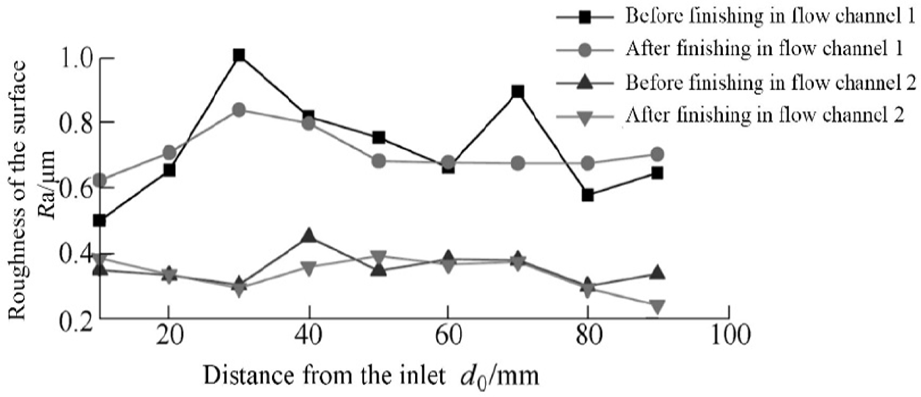
Roughness paralleled to the flow.

Figure 14.

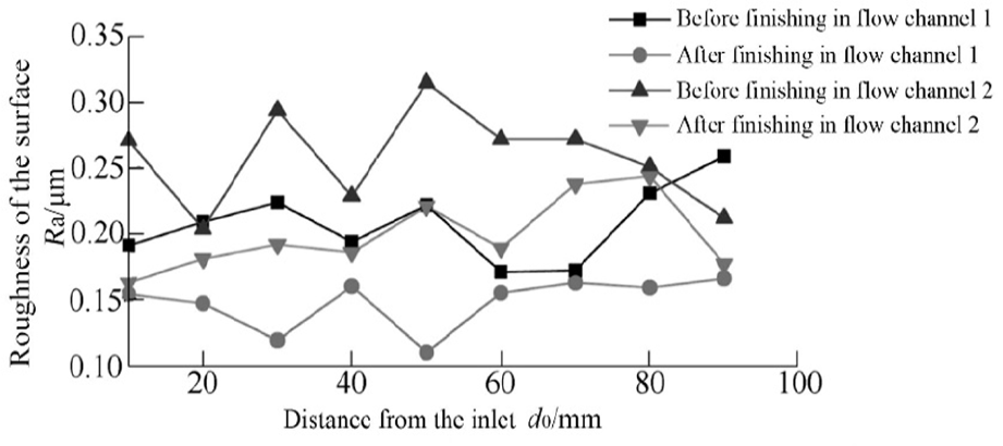
Roughness perpendicular to the flow.

To handle the contradiction between the high value of the roughness and the disappearance of the surface texture, the workpiece surface was photographed again by reducing the magnification. As shown in Figure 15, the rough machining texture is still visible. Each trace is measured at approximately 200 μm.

Figure 15.

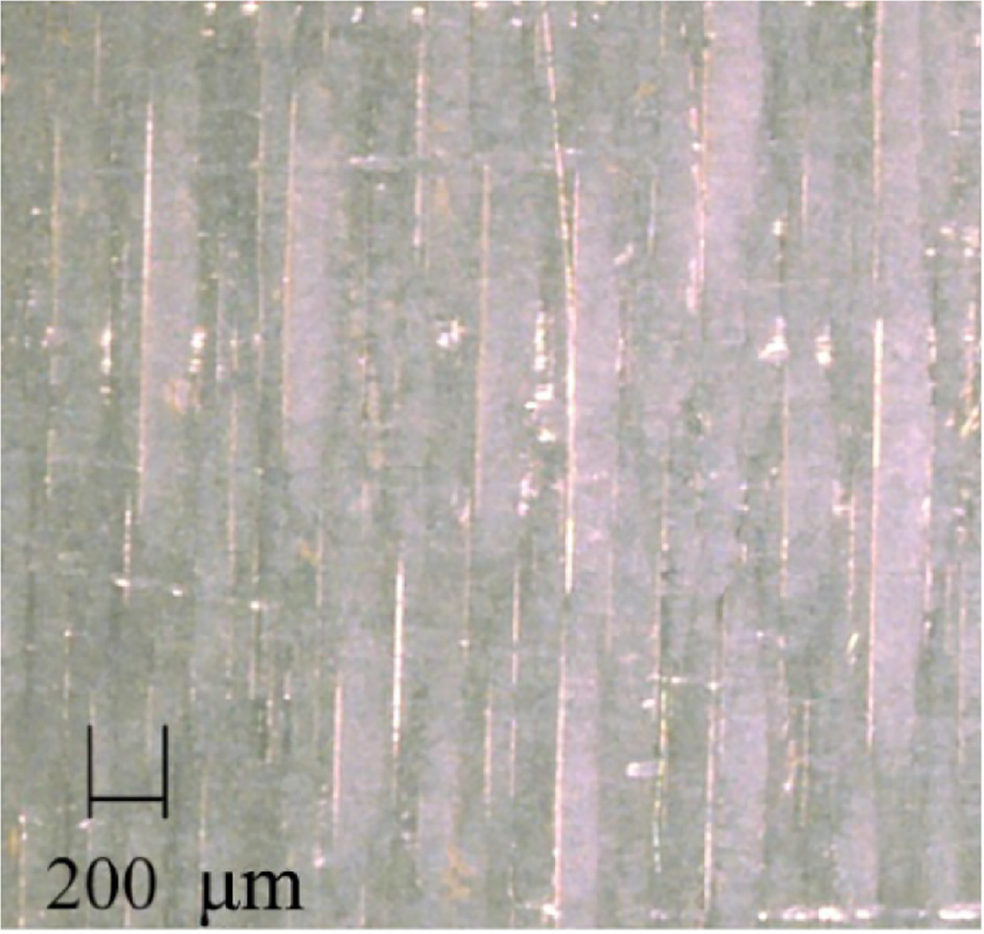
Flow 1 after machining the workpiece surface microphotos 50×.

Analysis of test results

Based on the Preston equation and another material removal model described in relation to the speed, pressure and the amount of material removal, the photo of the processed workpiece, and the painting tests confirmed that the volume fraction, the dynamic pressure, and the velocity field are the main parameters that determine the machining effect of the abrasive flow. The results also demonstrated that the wear debris obtained from the simulation of the abrasive particles can penetrate the boundary layer and the incident speed and the incident angle of the abrasive particles are consistent with the results of the machining test.

Traditional ultraprecision machining methods require machine tools with high stiffness and bearings with high cost. ¹ In addition, traditional methods are difficult to finish the inner walls of workpieces, especially those in small sizes. SAF is a good alternative.

The difference between surface roughness and microstructure is mainly caused by the characteristics of SAF and original surface texture. In this test, the contact roughness meter is used. The length of the sample is 0.8 mm, and the distance of the probe is 4 mm. The vibration amplitude of the workpiece is measured by the sliding of the probe on the surface of the workpiece to calculate the roughness. The surface texture of the raw workpiece machining showed that the cutter direction of rough grinding and fine grinding was perpendicular to each other, and they were respectively perpendicular and parallel to the flow direction of abrasive flow (Figure 12(a)). After 15-h machining, the marks of finishing were eliminated. However, the marks of rough finishing were reflected on the surface, resulting in an insignificant reduction in roughness, indicating that the parameters selected in this machining test were not suitable for the surface with excessive roughness due to the small amount of material removal. The original roughness of the workpiece should be below 0.2 μm, also indicating that the machining method should adopt a slight force and a small amount of cutting.

Conclusion

1. A boundary layer within the particle trajectory calculation model was established to calculate the impacting area, impacting velocity, and angle of incidence. By comparing the results, it was found that the surface area of the test workpiece corresponding to the incident area had an obvious processing effect in the simulation results so that the roughness in the area was less than that in the area without abrasive particles, demonstrating the feasibility of the trajectory calculation model.

2. The deflection of the flow around a constrained protrusion occurred. Under the influence of protrusions, both normal and spanwise vortices appeared in the flow field. Meanwhile, the vortices became larger due to the second and third protrusions so the fluid was obviously tilted to one side, which led to uneven dynamic pressure on the surface of the workpiece in the flow field.

3. CFD software simulation can calculate the flow field distribution in the constrained channel. Through the comparison of simulation and experiment results, it was found that the volume fraction of the abrasive particles and the dynamic pressure were important factors that affect the machining effect and the numerical value was related to the machining effect. Therefore, the numerical simulation method is feasible to predict the flow field and effect of SAF.

4. For the surface with excessive roughness and deep scratches, the machining by the SAF was not satisfactory because the pressure and fluid viscosity were not strong enough. In this experiment, the processing effect was obvious in the area with low original roughness, which is less than 0.2 μm. Therefore, suitable processing parameters should be selected according to the surface roughness of the original surface before processing.

5. The simulation results are consistent with the flow field distribution and machining effect so it can be used in the design of constrained modules. The parameters of the flow field—such as the velocity, angle of incidence, dynamic pressure, and volume fraction of abrasive particles—can be controlled according to the processing requirements to design the constrained modules. While ensuring the uniformity of the processing, the specific areas can be processed separately according to the requirements. The corresponding constrained module can be designed according to the form of the surface of the original workpiece to control the incidence direction of abrasive particles to reach the processing requirements.