Sage Journals: Discover world-class research

Abstract

Three-dimensional assembly process planning is a precondition for achieving full product lifecycle management based on three-dimensional modelling. Information expression and management operations of fixture models are key to three-dimensional assembly process planning systems. To reasonably and efficiently achieve the goal of planning assembly processes with a fixture model, the application of a fixture information model to a three-dimensional assembly process planning system is investigated. First, to manage tooling information, a fixture information model is defined that consists of management information, display information, geometric information, assembly constraints and degrees of freedom. Then, based on the analysis of the degrees of freedom of components and the assembly constraint relationship, a method of solving assembly constraints based on degrees of freedom reasoning is proposed. Finally, by using the method of solving assembly positioning based on geometric constraints, the pose transformation and assembly positioning of parts are achieved. Through the development of a tooling function module, the three-dimensional assembly process planning system is improved. The feasibility of the above method is verified using part of a spacecraft as an example.

Keywords

Three-dimensional assembly process fixture information model degrees of freedom reasoning assembly constraint solving assembly spatial pose solving

Introduction

Assembly is the last step of the product manufacturing cycle. Assembly is directly related to the final functioning and quality of products, so assembly has always been considered highly important in the manufacturing field. Practice has proven that assembly in the modern manufacturing industry uses the most time of all manufacturing processes. According to a survey conducted by Boothroyd,¹ assembly accounts for 20% to 70% of the total production workload. In addition, because of the large proportion of manual labour required in assembly work, assembly time accounts for 40% to 60% of the total product manufacturing workload. The product assembly cycle is longer for products with highly complex features requiring discrete manufacturing in the aerospace field, such as spacecraft and aircraft. Therefore, the development of assembly technology is an important method of guaranteeing the quality and function of products, which is of great significance in improving the product quality and reducing the cost and time of the design cycle.²

Complex products generally have a large number of components, complex assembly relationships, and require high assembly accuracy. To achieve more competitive product quality, the requirements of product assembly precision are becoming increasingly more strict.³ Traditional two-dimensional (2D) assembly process specifications have difficulty meeting the manufacturing requirements, and using digital methods to improve the efficiency of assembly process planning and assembly quality is an important development direction. The traditional 2D assembly process mainly uses computers to conduct assembly process planning, simulation and optimisation. Many research institutions have conducted in-depth research, developed assembly process prototype systems and explored a variety of assembly process planning methods. For example, Washington State University has developed a virtual assembly design environment (VADE),⁴ the first representative assembly process system in the world. However, most studies have focussed on the assembly process planning of present products. There has not been any systematic study of the application of product fixture in assembly process planning systems. As such, devices assist operators in completing assembly tasks; the fixture is also an important factor in the process of product assembly process planning and directly affects its accuracy and the reliability of assembly simulation verification.⁵ Because of this condition, our team developed function modules of tooling based on a self-developed assembly process planning prototype system for three-dimensional (3D) models.^6,7 We investigated the tooling part of product assembly process planning to enrich and improve the existing prototype system. The application of tooling model information in product assembly process planning was achieved, thus improving the efficiency of product assembly process planning.

The remainder of this article is structured as follows. The ‘Literature review’ section analyses related works. The ‘Fixture model in an assembly process system’ section introduces the structure of the fixture model and provides definitions related to our assembly process system. The ‘Assembly constraint solving and assembly positioning solving’ section presents our solutions for assembly constraint and assembly positioning. The ‘System application verification’ section describes module development and its implementation in our system. Finally, we conclude and outline future work in the ‘Conclusion and future work’ section.

Literature review

Our research on assembly tooling in assembly process planning unifies concepts from information model representation and assembly constraint location (including positioning and orienting). In this section, research related to these two areas of assembly tooling is described.

Assembly sequence planning

The essence of assembly sequence planning (ASP) is to find a reasonably feasible component sequence based on a given product assembly model, and ASP is a critical step of assembly planning in product digital manufacturing. It is a combinational optimisation problem with strong constraints.⁸ The ASP problem of a product is essentially a combinatorial optimisation problem. As the number of components in a product increases, the number of assembly sequences (including feasible and infeasible) will increase exponentially.

In the traditional method of ASP, Bourjault⁹ was the first to study ASP. He proposed the assembly precedence relations (APR) question and answer method, using the joint diagram to express the geometric model and assist to optimise the assembly sequence . He also proposed a priority relationship concept based on an assembly sequence, and the connection graph model was used to implement ASP, laying a foundation for the research of computer-aided ASP. Thomas L De Fazio and Daniel E Whitney¹⁰ optimised Bourjault’s method and changed his question form, but they needed to initially ask the user about the assembly priority, so the efficiency was reduced when getting the assembly sequence precedence. This method is only suitable for the case of fewer components, and the requirements for knowledge quality are relatively high.

The disassembly method then appeared, and the disassembly method was an indirect method for ASP . In general, assembly and disassembly of components are mutually reversible processes. Baldwin¹¹ used disassembly to address assembly problems and used Cut-Sets to solve assembly association diagrams to generate all assembly cuts. Although this method is very systematic, there is a combination explosion problem of the assembly sequence when the number of components is too large. To solve this problem, some researchers use the Cut-Sets method and the AO* algorithm (AND/OR graph heuristic search algorithm) to search for and evaluate the optimal assembly sequence.^12,13

De Mello and Sanderson proposed AND/OR graphs, by which the precedence of the parts can be exactly represented. Then, a few methodologies were developed for the AND/OR graph.^14,15 After considering the assembly time and physical constraints, many related works have been performed.¹⁶ These methods have reduced the time required to search assembly sequences and can provide complete and correct feasible sequences. However, the optimal solution cannot be obtained.

In addition, genetic algorithm (GA) has been implemented to address the problem that is the most common optimisation technique. Simulated annealing, ant colony algorithm (ACA) and particle swarm optimisation (PSO) techniques are most used next to GA.¹⁷ Several other optimisation techniques also have been successful in solving ASP.^18,19 The artificial intelligent methods have several limitations such as localised search and high computational time; hence, the resulting sequence is a near optimal assembly sequence but not the global optimised sequence. Besides these limitations, predicate considerations/assumptions slightly reduce the complexity of the problem but highly affect the search space and lead to higher time consumption and skilful user interventions.

All these methods are simple schemes and easy to use. However, there is still an issue that needs to be addressed. The tool constraint relationships have rarely been studied. In fact, because the assembly process tools are usually used, it is critical to add the analysis of the tool constraint relationship to the assembly model.

Li et al. were the first to consider the assembly resources. Cheng Hui et al.²⁰ combined the GA and the ACA, where the codes represent the assembly parts and assembly resources and chromosomes represent the assembly sequence. The iterative method was used to obtain the final assembly sequence, but the shortcomings of this method are that the interference of the assembly and assembly resources is not considered and the fitness function does not consider the feasibility of assembling the resource direction. Sun et al.²¹ constructed the information matrix of assembly resource state and combined the weighting coefficients to form the fitness function by combining the assembly resource constraints, geometric feasibility of the assembly sequence, stability of the sub-assembly and number of assembly redirection. The effectiveness of the method is verified by GA. Although they consider the feasibility of the assembly direction, they do not get the assembly sequence of the assembly resources.

Information model representation of assembly tooling

The representation of an assembly tooling information model is part of assembly process planning. Assembly tooling plays an important role in guaranteeing the required location and orientation of sub-assemblies and parts.²² Because assembly resources can identify and solve problems such as component assembly interference or unreasonable assembly sequence in advance, assembly tooling information models can be integrated into assembly process modelling. In virtual assembly or computer-aided assembly process planning, many researchers have investigated the representing and modelling of assembly tooling information.

In a self-developed VADE system, Washington State University⁴ proposed models of hand-tool and tool-part interaction. These models were used to operate the tools and complete assembly tasks. Phong and Simmy²³ proposed a simple data model for assembly process planning and analysed the effect of assembly tools on assembly processes by defining their related parameters. Kang²⁴ proposed a solution which is used for assembly and disassembly tool management, positioning and simulating assembly processes. By introducing a point vector model, the features of tool positioning and operation could be represented, providing information support for assembly tool positioning. Hongmin et al.²⁵ proposed an interactive assembly tool planning based on an assembly semantic model. By using the assembly semantic processing method, such as recognition, solving and navigation, a series of methods, including assembly tool selection, orientation and manipulation, are proposed. However, the tool model library is not rich enough. Raju Bahubalendruni et al.²⁶ proposed a tool-based bounding box method to solve geometrical feasibility using a practically feasible optimal ASP. Assembly tools were classified into three main types based on their application in assembly development, namely, Pre tools, In tools and Post tools.

Because the assembly resources can improve the feasibility and efficiency of the assembly sequence in the actual assembly, there are large differences in the structure, materials and volume of the components to be assembled, and there are many types of tools required. Because assembly resources can be complicated, there are many attempts at creating a tool library, but a relatively complete tool library has not been established, and there is a distance from the actual application.

Assembly constraint location of assembly tooling

The constraint positioning process in assembly tooling is essentially a problem of geometric constraints. The specific process is to (1) determine the space target matrix according to the assembly tool geometric constraints, (2) adjust the spatial pose of the assembly tools and (3) achieve the rapid navigation and positioning of the assembly tools. To solve the geometric constraints between two rigid bodies, there are several representative methods that can be classified into four categories: numerical methods, symbolic algebra methods, rule-based methods and graph-based methods.^27,28 In practical applications, several methods are often used in combination to achieve better results. The rule-based geometric constraint method can be used to adopt an inference mechanism to solve geometric constraints. In addition, this method does so by constructing constraint-solving rules, and is easy to implement and has good stability. The degree of freedom (DOF) analysis, one of the rule-based geometric constraint methods, plays a dominant role in the positioning of the 3D part assembly.

Qiao et al.²⁹ proposed an inference solving method based on DOF analysis. Through the intersection of the remaining DOF space and degrees of constraint (DOC) space, the DOF could be reduced. Then, the assembly positioning of parts is realised by implementing rotational and translational transformation in the remaining DOF space. The advantage of the rule-solving method is that it is easy to implement the solution. The disadvantage is that it is limited by the rules itself, the implementation efficiency is low and the constraint closed-loop problem cannot be handled. In terms of intelligent algorithms, Wei and Xiaogang³⁰ adopted a PSO algorithm based on geese to solve the geometric constraint problem. The constraint equations of geometric constraint problems are transformed into optimisation models, and the problem of constraint solving is translated into an optimisation problem. Cao et al.³¹ proposed a quantum GA that combines GA and quantum theory using the double-strand quantum chromosome structure to achieve the crossover operation of the GA using quantum gate transformation. The comparison of non-linear equations and geometric constraints with other methods shows that the algorithm for solving geometric constraint problems has better accuracy and solving rate. The problem with intelligent algorithms is that they require multiple inputs and are limited by knowledge.

Zhang et al.³² proposed an assembly constraint hierarchical model and dynamically built the constraints of a virtual assembly system based on DOF analysis. All operating objects can be reasonably located by constraint navigation technology in the virtual environment. This method can guide the movement process according to the constraints that the components satisfy but does not meet the intention of the designer in the process of solving for the actual amount of rotation. Hongmin et al.²⁵ proposed an interactive assembly tool orientation based on assembly semantic reasoning and collection detection. The orientation makes the assembly orientation process visual and more efficient than that based on geometric reasoning, and can support interactive assembly tool manipulation simulation and can easily solve the operation space reasoning.

The literature review shows that there are many studies and applications on solving assembly constraints and positioning components and tools in virtual assembly processes. However, the application of fixtures is less well studied and applied to assembly constraints in assembly process design and simulation. At the same time, there are few systematic and in-depth studies on information models of assembly fixture from the aspect of assembly fixture positioning and movement navigation. At present, commercial computer aided design (CAD) systems such as NX UG, Creo Parametric (previously Pro/Engineer Wildfire) and SolidWorks have relatively complete modules for assembly positioning and geometric constraint solving. However, these systems use assembly constraint methods based on points, edges and faces, which differ from the assembly constraint solutions used in virtual assembly and assembly process design. Therefore, in the self-developed 3D assembly process design software AMT Processor,^7,33 the representation of assembly fixture information model, algorithm of solving spatial pose and assembly positioning solving of assembly fixture based on the DOF reasoning are systematically expounded in the next section.

Fixture model in an assembly process system

Expression of the fixture information model

In assembly process planning systems, a conversion interface is used to read 3D model process files designed by 3D CAD software. The interface then extracts valid information from the files and adds other necessary information before generating a fixture information model. This is the method of generating an assembly tooling information model. Fixture models include management information, display information, geometry information, assembly constraints and DOF information, as shown in Figure 1. What needs to be explained is that the geometric model includes a series of geometric elements such as points, lines and surfaces. Geometric surfaces are the main assembly features. Therefore, the geometric elements involved in the constraint are various types of geometric surfaces, including planes, cylinders and cones. When an assembly constraint is imposed on a geometric model, geometric constraints are actually imposed on each of the geometric surfaces involved in the assembly.

Figure 1.

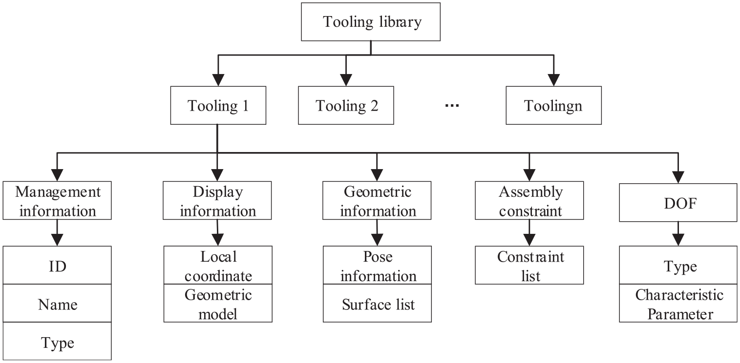
Expression of the fixture information model.

Management information

Fixture management information includes data such as identification number (ID), name and type. The ID represents the unique number of the fixture, the name is the name of the fixture and the type is the type of fixture according to its usage scope, such as common fixture, special fixture and standard fixture.

Display information

Fixture display information consists of local coordinates and a geometric model. Local coordinates represent the local coordinate system where the parts are located, while the geometric model represents the patch display information of the parts in the model view area, which is also the solving object and carrier of assembly constraints. A geometric model of the part provides the information necessary for assembly. The part’s geometric model can be expressed as

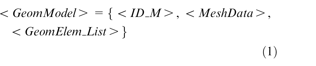
< G e o m M o d e l > = {< I D_M >, < M e s h D a t a >, < G e o m E l e m_L i s t >}

(1)

where ID_M is the ID of the geometric model of the part; MeshData represents the part’s data displayed in the model view area, which is obtained after discretisation and mesh treatment of the part’s precise geometric data in the design document, and MeshData helps to save computer storage space and improve operational efficiency; and GeomElem_List represents the list of geometric elements which correspond to the geometric model. The geometric element list here refers to the surface list.

Geometric information

Geometric information consists of pose information and a surface list. Pose information describes the position and orientation of components in terms of a global coordinate system. The surface list represents the part’s geometric surface list. The assembly of parts is usually achieved by using a constraint relationship between geometric surfaces. Therefore, geometric elements can be expressed as

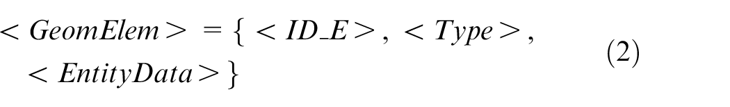
\begin{matrix} < GeomElem > = {< ID_E >, < Type >, \\ < EntityData >} \end{matrix}

(2)

where ID_E represents the identification of geometric elements, Type represents the type of geometric element, and EntityData represents precise geometric data. Geometric elements here represent geometric surfaces.

Assembly constraints

Assembly constraints consist of a set of geometric constraints. Geometric constraints are constraint relationships imposed on the geometrical surfaces of the parts. Geometric constraints are the core objects of constraint solving and are the basis of component positioning. They are also used to determine the assembly relationships between components. Therefore, it is crucial to describe the geometric constraint information to facilitate constraint solving. Geometric elements are the direct carriers of geometric constraints, the geometric model corresponds to a list of geometric elements, the part’s geometric model is an indirect carrier of geometric constraints, and geometric models and geometric elements are the basic elements of constraint information. When applying constraints to geometric elements, recording the constraint type is necessary. Therefore, geometric constraints can be expressed as

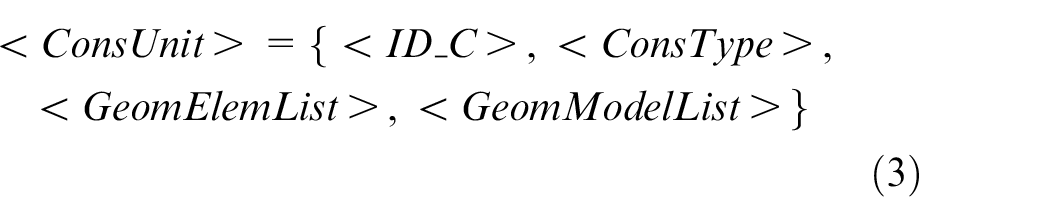
\begin{matrix} < ConsUnit > = {< ID_C >, < ConsType >, \\ < GeomElemList >, < GeomModelList >} \end{matrix}

(3)

where ID_C represents the unique ID of the geometric constraints, ConsType represents the type of constraint, GeomElemList represents two geometric elements involved in the constraint, and GeomModelList represents two-part geometric models corresponding to GeomElemList.

DOF information

The characteristic parameter is a parameterised expression of the DOF category and describes the freedom space (FS) of the components. The DOF information can be expressed as

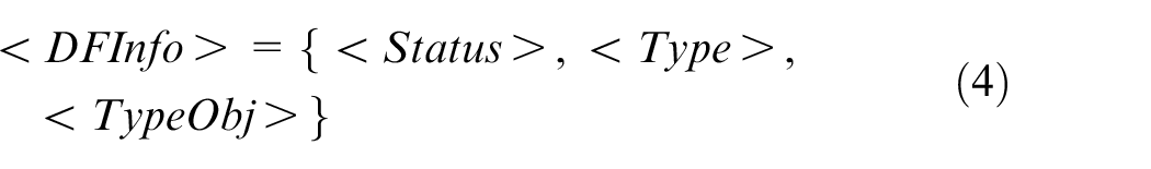
\begin{matrix} < DFInfo > = {< Status >, < Type >, \\ < TypeObj >} \end{matrix}

(4)

where Status represents the status of DOF, whose value is 1 or 0. If Status = 0, the part to be assembled is completely free. If Status = 1, the part is in a state of constraint. Type represents the category of DOF, TypeObj is a category object, which is the parameter expression of DOF. The category of DOF and its parameter expression are introduced in the following DOF analysis.

Geometric models and the geometric elements of parts

Design files usually contain the method of generating part features and precise geometric and topological information to meet the design needs of users. In the fixture module, the main purpose of part geometric models is to provide data to display the part in the model view area, display the assembly relationships of the components in the view area and associate precise geometric elements. Therefore, the part geometric model does not need to contain all of the information in the design files. Instead, the information can be obtained by performing patch processing on solid geometric data and filtering the feature generation method and other information through the conversion interface, greatly saving system memory and improving system operation efficiency.

The essence of part assembly is to impose constraints on the geometric elements and adjust the pose of the part model according to the constraint relationships to achieve assembly. Therefore, in the fixture module, the main role of the geometric elements is to participate in geometric constraint solving as elements of geometric constraints according to the constraint relationship. There are mainly point–line, point–surface, line–line, line–surface and surface–surface constraints between geometric elements. Geometric surfaces are the main assembly features in physical entities. Therefore, in the fixture module, the geometric elements involved in the constraint include various types of geometric surfaces, mainly including planes, cylinders and cones. This article focuses on the geometric constraints between geometric surfaces. Unless special instructions are given, geometric elements only represent the geometric surfaces. Common constraints between geometric surfaces include (1) constraints between two planes, (2) constraints between a plane and cylinder, (3) constraints between two cylindrical surfaces, (4) constraints between cylindrical and conical surfaces and (5) constraints between two conical surfaces.

In the model view area, constraint elements are chosen to apply constraints. Geometric model information in the view area is not accurate and cannot be used for assembly constraint solving. Therefore, to obtain accurate geometric data, it is necessary to make the geometric elements correspond to the information of the geometric model. The relationship between the geometric model and the geometric elements is shown in Figure 2.

Figure 2.

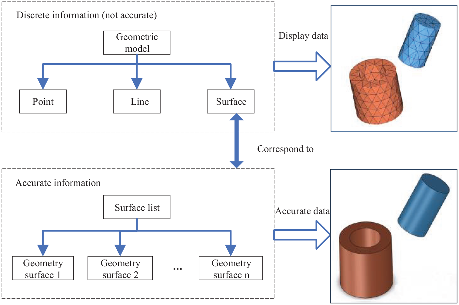
Diagram of the relationship between the geometric model and geometric elements.

Assembly constraints and geometric constraints

Common types of geometric constraints include (1) coincidence, (2) parallelism, (3) verticality, (4) tangency, (5) coaxiality, (6) distance and (7) angle. A set of geometric constraints on the components forms the assembly constraints. The geometric constraints are the basic units of the part assembly constraints, assembly constraints and geometric constraints, as shown in Figure 3.

Figure 3.

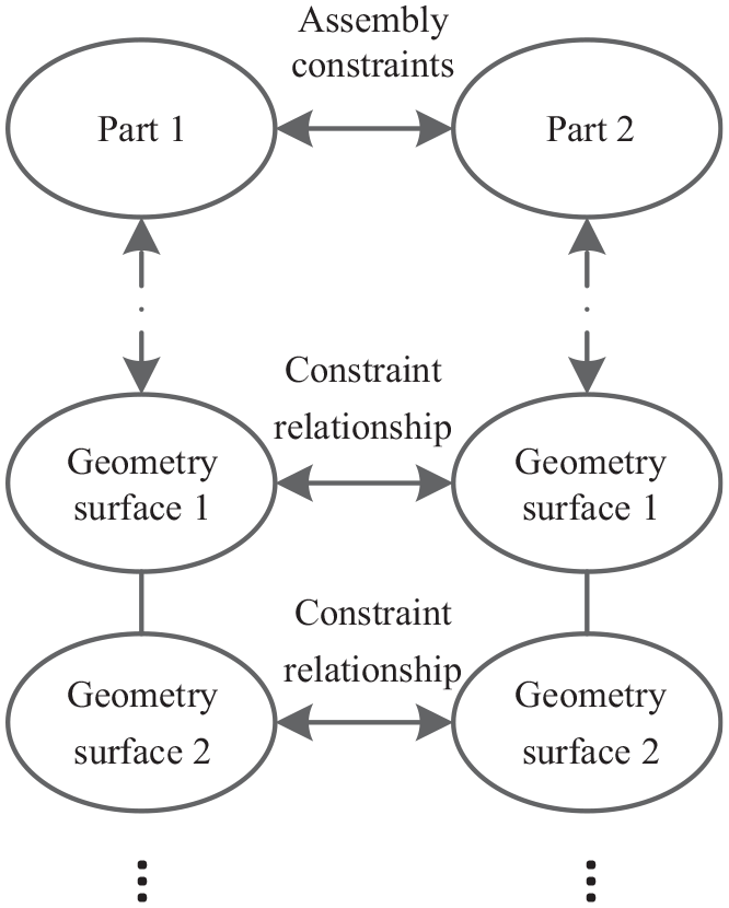
Diagram of the relationship between assembly constraints and geometric constraints.

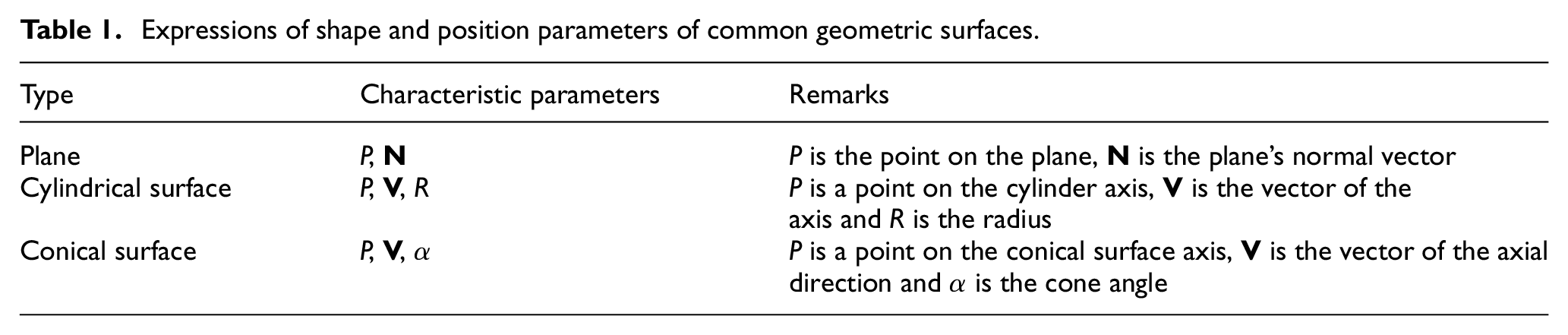
Expression of the shape and position of fixture geometric elements

In the fixture module, the assembly of the fixture is achieved through changes to the poses of the parts to be assembled. Such changes are achieved by the geometric element constraints on the two parts. To facilitate constraint solving, the geometric elements can be expressed by using characteristic parameters. For example, a plane can be expressed as the centre of a surface and its normal vector, while a cylindrical surface can be expressed as the vector of an axis, a point on the axis and the radius of the circle. Table 1 shows expressions of the shape and position parameters of common geometric surfaces in the local coordinate system.

Table 1.

Expressions of shape and position parameters of common geometric surfaces.

Type	Characteristic parameters	Remarks
Plane	P, N	P is the point on the plane, N is the plane’s normal vector
Cylindrical surface	P, V, R	P is a point on the cylinder axis, V is the vector of theaxis and R is the radius
Conical surface	P, V, $α$	P is a point on the conical surface axis, V is the vector of the axialdirection and $α$ is the cone angle

Assembly constraint solving and assembly positioning solving

Assembly constraint solving based on DOF inference

The assembly constraints between two parts appear as geometric constraints between the geometric elements of the two parts. Assembly constraint solving must satisfy the new geometric constraint relationship without violating the original one. The assembly constraint can be solved by recording, analysing and reasoning the DOF information of the part according to the geometric constraint relationship.

Relationship between DOF and constraints

Without constraints, the DOF of each part can be decomposed into three degrees of rotational freedom (DRF) and three degrees of translational freedom (DTF). The FS is the entire 3D space. When the part is constrained, the DOF of the part is limited, and the process of satisfying constraints is a process of decreasing the DOF of the part. Constraints and DOF are a pair of contradictions interacting with each other. When adding constraints, the DOF of the part decreases. When the constraints are eliminated, the DOF of the parts increases.

To facilitate the analysis of DOF, the relationship between the remaining degrees of freedom (RDF) and the constraints, and the relationship between the remaining freedom space (RFS) and constraint space (CS) are expressed as follows:

1. Relationship between RDF and DOC: This relationship can be expressed as

RDF = DF - DC

(5)

where DF represents the DOF. DC describes the degree of constraint on a part. DC = DTC + DRC, where DTC represents the degree of translational constraint and DRC represents the degree of rotational constraint.

RDF is the DOF of the part after it is constrained. RDF = RDTF + RDRF, where RDTF represents the remaining degrees of translational freedom and RDRF represents the remaining degrees of rotational freedom.

2. Relationship between RFS and CS: This relationship can be expressed as

RFS = FS - CS

(6)

where CS is the restriction that constraints impose on the FS of a part. CS = TCS + RCS, where TCS represents the translational constraint space and RCS represents the rotational constraint space.

RFS is RFS = RTFS + RRFS, where RTFS represents the remaining translational freedom space and RRFS represents the remaining rotational freedom space.

DOF analysis

The purpose of DOF analysis is to obtain the RDF of the part and the RFS under the constraints so as to facilitate geometric constraint solving. The process is as follows. (1) The RDF of a part is obtained before the new geometric constraint is imposed (when the part is unconstrained, the RDF is 6, which is in the completely free state). (2) The new constraint is applied through the analysis of the constraint relationship. The restriction is judged so the constraint bears on the DTF and DRF. (3) The RDF is calculated to obtain the RFS. Thus, geometric constraint solving is based on DOF analysis, and the satisfaction of the constraint relationship can be obtained through recording, analysing and reasoning the part DOF.

Analysis of the constraint relationship is a precondition for DOF analysis. In order to obtain the DC of each constraint relationship and the corresponding RDF, common types of constraint relationships needed to be analysed. According to Euler’s theorem, the motion of any part can be decomposed into rotation around an axis and translational in a direction. When movement is limited, there are four types of rotational part movement: non-rotation, rotation around a direction, rotation around a fixed point and free rotation. In addition, there are four types of translational movement: non-translation, translational in a direction, translational in a plane and free translation. According to part movement characteristics, the DOF expression of components is as presented in Figure 4, and common types of constraints and DOF analysis are shown in Table 2.

Figure 4.

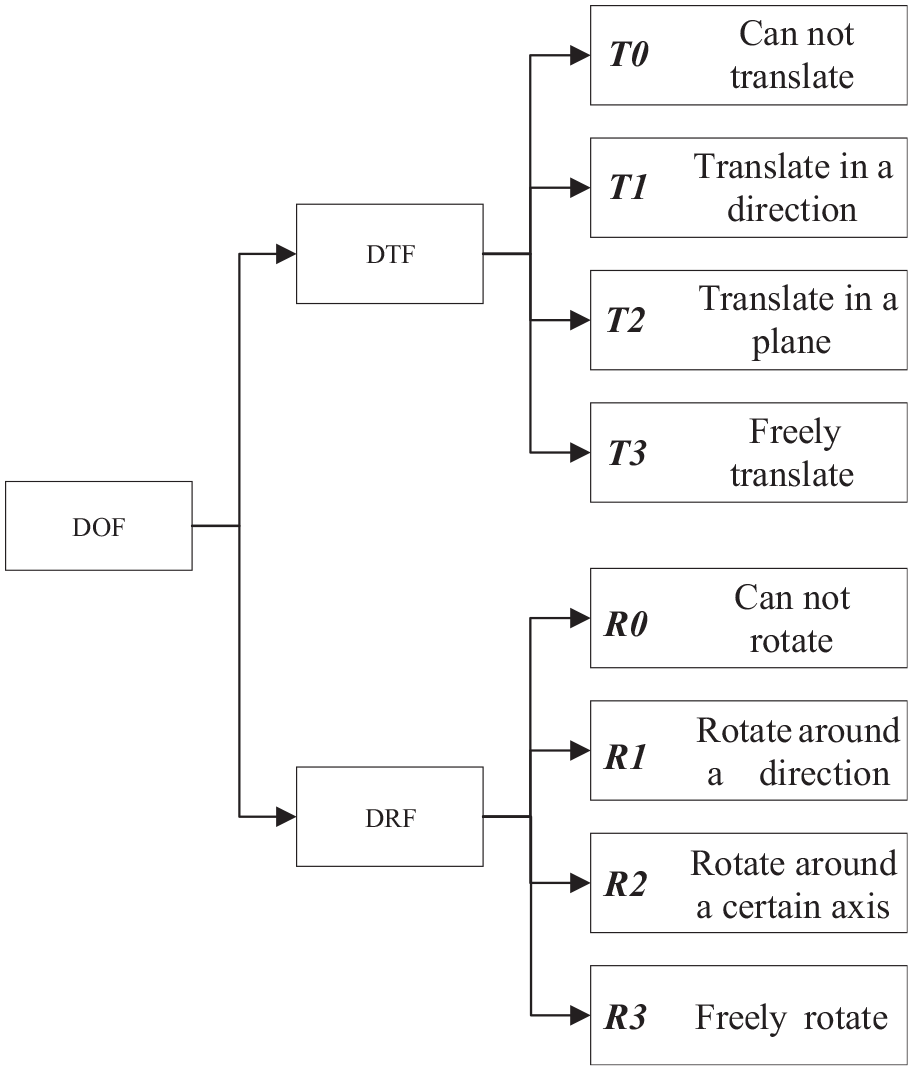
DOF expression of components.

Table 2.

Common types of constraints and DOF analysis.

Types of constraints	Geometric elements	(DTC, DRC)	(RDTF, RDRF)
Coincidence	Plane–plane	(1, 2)	(T2, R1)
Parallelism	Plane–plane	(0, 2)	(T3, R1)
Verticality	Plane–plane	(0, 2)	(T3, R1)
Tangency	Plane–cylindrical surface	(1, 2)	(T2, R1)
Coaxiality	Rotating surface–rotating surface	(2, 2)	(T1, R1)
Distance	Plane–plane	(1, 2)	(T2, R1)
Angle	Plane–plane	(0, 2)	(T3, R1)

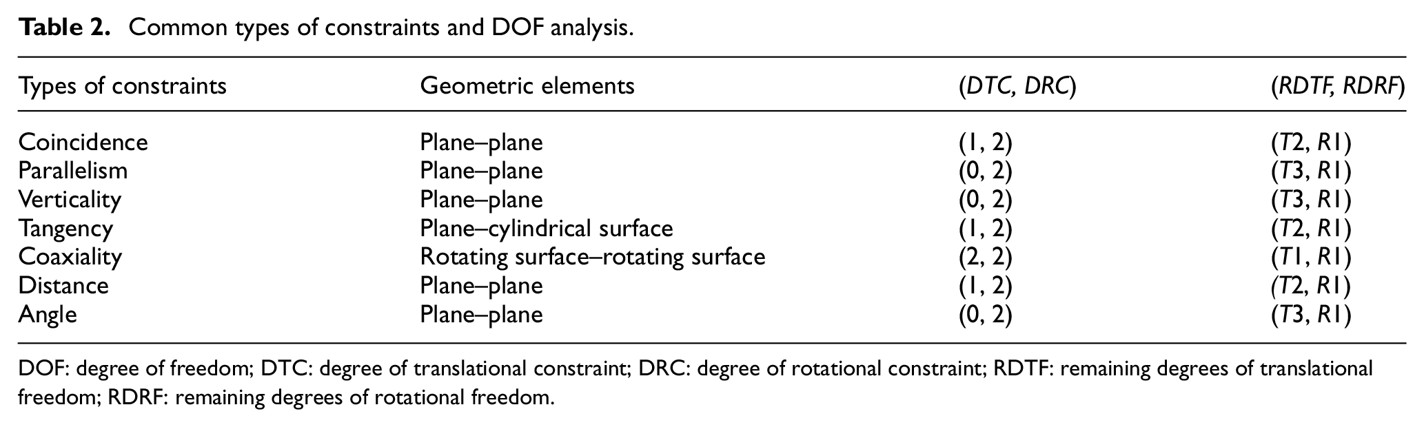
DOF: degree of freedom; DTC: degree of translational constraint; DRC: degree of rotational constraint; RDTF: remaining degrees of translational freedom; RDRF: remaining degrees of rotational freedom.

Shape and position expression of FS

Based on the DOF analysis, the relationships between the type and DC and the RDF are described, and the type of DOF of the part under the constrained condition is obtained. However, this is not enough to support the realisation of system functions. To facilitate system implementation, the RFS of the part needs to be mathematically described according to the types of DOF.

In general, the DRF and the DTF are described separately as follows.

1. RDTF

The DTF can be expressed as

RTFS (Type) = {pt, \vec{dir}}

(7)

where Type is the type of RDTF, pt represents a point and $\vec{dir}$ represents a vector. For different Types, pt and $\vec{dir}$ have different meanings. The shape and position expressions of translational FS are shown in Table 3.

2. RDRF

The DRF can be expressed as

R R F S (T y p e) = {p t, \vec{dir} 1, \vec{dir} 2}

(8)

where Type is the type of RDRF, pt represents a point and $\vec{dir} 1, \vec{dir} 2$ represent two vectors. For different Types, pt, $\vec{dir} 1$ and $\vec{dir} 2$ have different meanings. The shape and position expressions of rotational FS are shown in Table 4.

Table 3.

Shape and position expressions of translational FS.

Type of DOF	Pt	$\vec{dir}$
T0	The point does not exist	The translational axis vector does not exist
T1	A point on the straight line	Direction vector of the straight line
T2	A point on the plane	Normal vector of the plane
T3	Any point in space	Arbitrary rotation vector

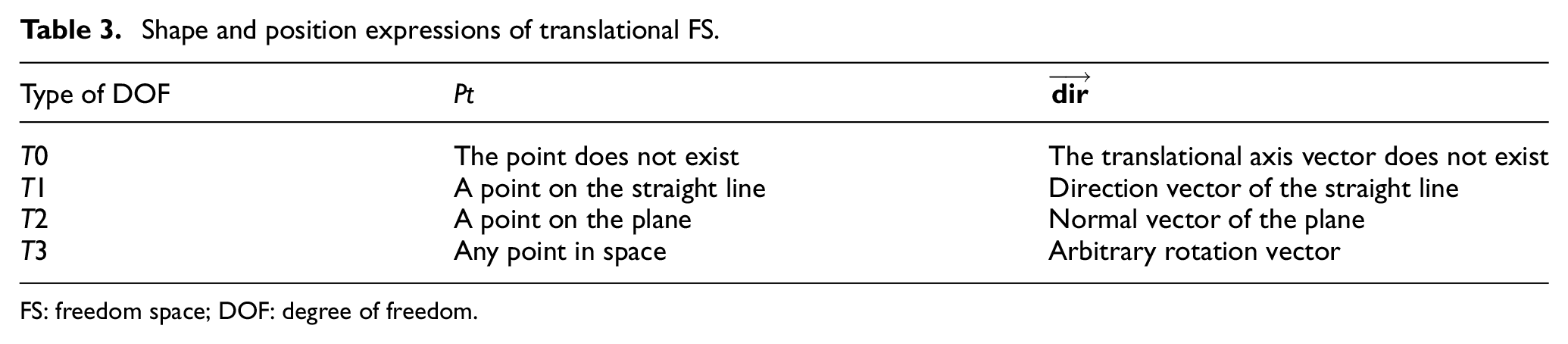
FS: freedom space; DOF: degree of freedom.

Table 4.

Shape and position expression of rotational FS.

Type of DOF	pt	$\vec{dir} 1$	$\vec{dir} 2$
R0	The point does not exist	Vector of rotational axis does not exist	Vector of rotational axis does not exist
R1	Any point	Direction vector of the rotational axis	Direction vector of the rotational axis
R2	A point on the axis of rotation	Direction vector of the rotational axis	Direction vector of the rotational axis
R3	Any point in space	Arbitrary vector of the rotational axis	Arbitrary vector of the rotational axis

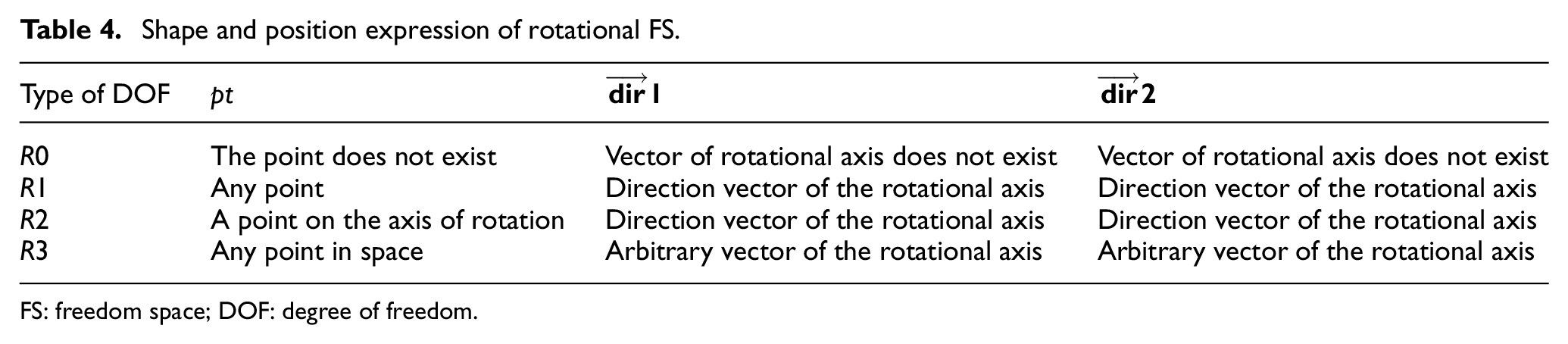
FS: freedom space; DOF: degree of freedom.

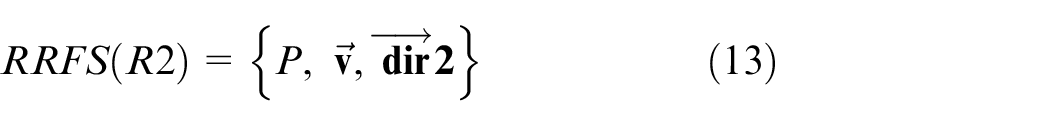
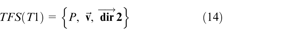
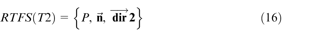
For specific constraints, mathematical methods are used to describe the RFS. There are two types of geometric constraint relationships, one is distance and the other is angel. Among them, constraints of distance type refer to distance constraint relationships between two planes, such as coincidence and distance. Constraints of angel type refer to an angle constraint relationship between two planes, such as parallelism, verticality and angle.

1. Distance constraints

For distance constraints, as shown in Figure 5(a), the distance between Surface A-1 on Part A (to be mounted) and Surface B-1 (on the reference Part B) is d (if d = 0, the plane coincides); $\vec{n}$ is the normal vector of Surface A-1, and P is a point on the plane. Then, the RRFS of Part A can be expressed as

RRFS (R 1) = {pt, \vec{n}, \vec{dir} 2}

(9)

where pt and $\vec{dir} 2$ do not exist.

The remaining freedom translational space can be expressed as

RTFS (T 2) = {P, \vec{n}, \vec{dir} 2}

(10)

where $\vec{dir} 2$ does not exist.

2. Angle constraints

For angle constraints, as shown in Figure 5(b), the angle between Surface C-1 on Part C (to be mounted) and Surface D-1 (on the reference Part D) is $θ$ ; $\vec{n}$ is the normal vector of Surface C-1, and P is a point on the plane. Then, the RRFS of Part C can be expressed as

RRFS (R 1) = {pt, \vec{n}, \vec{dir} 2}

(11)

In the formula, pt and $\vec{dir} 2$ do not exist. The remaining translational FS of part A can be expressed as

RTFS (T 3) = {pt, \vec{dir} 1, \vec{dir} 2}

(12)

In the formula, pt is an arbitrary point, while $\vec{dir} 1$ and $\vec{dir} 2$ are arbitrary vectors.

3. Coaxiality constraints

For coaxiality constraints, as shown in Figure 5(c), Surface E-1 on Part E (to be mounted) and rotational Surface F-1 (on the reference Part F) are coaxial; $\vec{v}$ is the direction vector of the axis of the rotation surface A-1, and P is a point on the axis. Then, the RRFS of Part E can be expressed as

RRFS (R 2) = {P, \vec{v}, \vec{dir} 2}

(13)

where $\vec{dir} 2$ does not exist.

The remaining translational FS can be expressed as

TFS (T 1) = {P, \vec{v}, \vec{dir} 2}

(14)

where $\vec{dir} 2$ does not exist.

4. Verticality constraints

For verticality constraints, as shown in Figure 5(d), Surface G-1 on Part G (to be mounted) and rotational Surface H-1 (on the reference Part H) is vertical; $\vec{n}$ is the normal vector of Surface G-1, P is a point on the plane and $\vec{v}$ is the direction vector of the axis of the rotation Surface H-1. Then, the RRFS of Part G can be expressed as

RRFS (R 1) = {pt, \vec{n}, \vec{v}}

(15)

where pt does not exist.

The remaining translational FS can be expressed as

RTFS (T 2) = {P, \vec{n}, \vec{dir} 2}

(16)

where $\vec{dir} 2$ does not exist.

Figure 5.

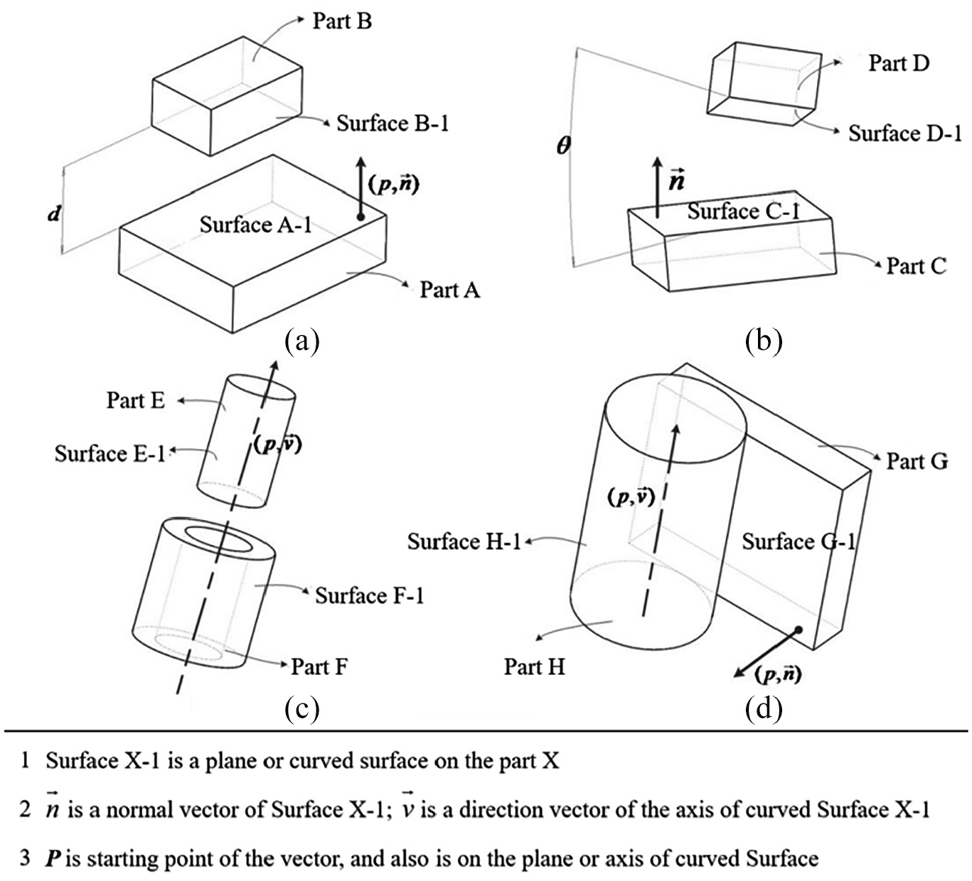
Shape and positional expressions of FS.

DOF reasoning

When a part is assembled, its position and orientation are determined by solving the assembly constraints. According to the above, the assembly constraints are usually composed of a combination of multiple geometric constraints. In order to solve the assembly constraints, the DOF of the parts must be inferred according to the geometric constraints. That is, in the case that the original constraints are not broken and the new constraints are met, the DOF of the part is updated. Because of the independence of translational constraints and rotational constraints, DOF reasoning can be divided into translational DOF reasoning and rotational DOF reasoning.

DTF reasoning

The RDTF and the DTC can be described as RDTF = RDTF – DTC. To facilitate understanding of the reasoning of the DTF, the following assumptions are made.

1. Current RDTF

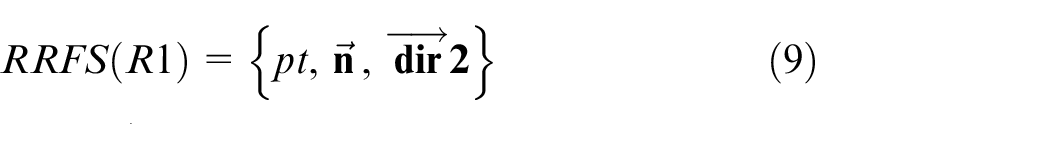
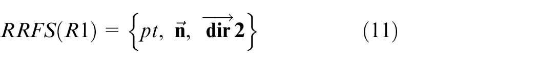
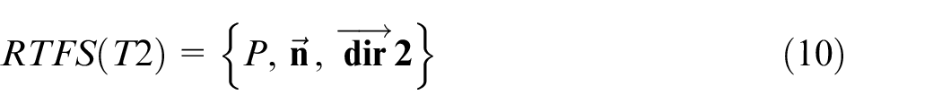
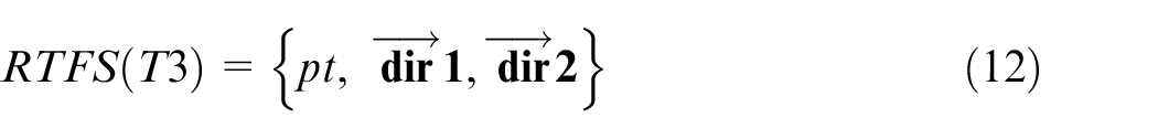
Assuming that the current RDTF of the part to be mounted is T2, then the characteristic parameters of the remaining translational FS are expressed as ( $P'$ , $\vec{N}'$ ), where $P'$ is a point on the plane and $\vec{N}'$ is the normal of the plane. If the current RDTF is T1, then the characteristic parameters of the remaining translational FS are expressed as ( $P'$ , $\vec{V}'$ ), where $P'$ is a point on the axis and $\vec{V}'$ is the direction vector for the axis.

2. The newly imposed translational constraint.

Assuming that the degree of the newly introduced translational constraint of the part to be installed is 1, the characteristic parameters of the remaining translational FS are (P, $\vec{N}$ ), where P is a point on the plane and $\vec{N}$ is the normal of the plane. If the newly introduced degrees of translational constraint are 2, then the characteristic parameters of the remaining translational FS are expressed as (P, $\vec{V}$ ), where P is a point on the axis and $\vec{V}$ is the direction vector for the axis.

Afterwards, through the enumeration method, the reasoning criteria of the DTF are given, as shown in Table 5.

Table 5.

Reasoning criteria for the DTF.

Type of constraint	Degrees oftranslationalconstraint	RDTF
Type of constraint	Degrees oftranslationalconstraint	T3	T2	T1	T0
Non-existence	0	T3	T2	T1	T0
Coincidence	1	T2	If $\vec{N}$ and $\vec{N}'$ are collinear, then it is T2If $\vec{N}$ and $\vec{N}'$ are not collinear, then it is T1	If the plane defined by (P, $\vec{N}$ ) is parallel to $\vec{V}'$ then it is T1; otherwise, it is T0	T0
Parallelism	0	T3	T2	T1	T0
Verticality	0	T3	T2	T1	T0
Tangency	1	T2	If $\vec{N}$ and $\vec{N}'$ are collinear, then it is T2If $\vec{N}$ and $\vec{N}'$ are not collinear, then it is T1	If the plane defined by (P, $\vec{N}$ ) is parallel to $\vec{V}'$ , then it is T1; otherwise, it is T0	T0
Coaxiality	2	T1	If $\vec{V}$ is parallel to the plane defined by ( $P'$ , $\vec{N}'$ ), then it is T1; otherwise, it is T0	If $\vec{V}$ and $\vec{V}'$ are collinear, then it is T1; otherwise, it is T0	T0
Distance	1	T2	If $\vec{N}$ and $\vec{N}'$ are collinear, then it is T2If $\vec{N}$ and $\vec{N}'$ are not collinear, then it is T1	If the plane defined by (P, $\vec{N}$ ) is parallel to $\vec{V}'$ , then it is T1; otherwise, it is T0	T0
Angle	0	T3	T2	T1	T0

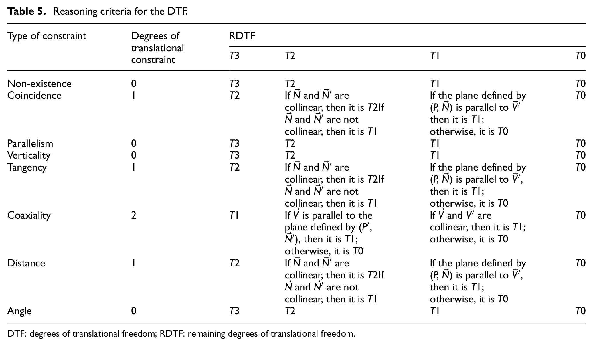
DTF: degrees of translational freedom; RDTF: remaining degrees of translational freedom.

DRF reasoning

The reasoning for the RDRF of the part and the DRC can be expressed as RDRF = RDRF – DRC. To facilitate understanding of RDRF reasoning, first make the following assumptions.

1. Current RDRF.

Assuming that the current RDRF of the part to be mounted is R2, then the characteristic parameters of the RRFS are expressed as $L' = (P', {\vec{V}}^{'})$ , where $P'$ is a point on the rotation axis $L'$ , and $\vec{V}'$ is the direction vector of the rotational axis $L'$ . If the current RDRF is R1, then the characteristic parameters of the RRFS are expressed as $l' = \vec{V}'$ , where $\vec{V}'$ is the direction vector of the rotational axis $l'$ .

2. Newly imposed rotation constraint.

Assuming that the newly introduced degrees of the rotational constraint of the part to be installed is 2, then the characteristic parameters of the RRFS are expressed as $L = (P, \vec{V})$ or $l = \vec{V}$ , where P is a point on the axis and $\vec{V}$ is the direction vector for the rotational axis.

Then, through the enumeration method, the reasoning criteria for the DRF are given, as shown in Table 6.

Table 6.

Reasoning criteria of DRF.

Type of constraint	Degrees of rotational constraint	RDRF
Type of constraint	Degrees of rotational constraint	R3	R2	R1	R0
Non-existence	0	R3	R2	R1	R0
Coincidence	2	R1	If l and $L'$ are collinear, then it is R2; otherwise, it is R0	If l and $l'$ are collinear, then it is R1; otherwise, it is R0	R0
Parallelism	2	R1	If l and $L'$ are collinear, then it is R2; otherwise, it is R0	If l and $l'$ are collinear, then it is R1; otherwise, it is R0	R0
Verticality	2	R1	If l and $L'$ are collinear, then it is R2; otherwise, it is R0	If l and $l'$ are collinear, then it is R1; otherwise, it is R0	R0
Tangency	2	R1	If l and $L'$ are collinear, then it is R2; otherwise, it is R0	If l and $l'$ are collinear, then it is R1; otherwise, it is R0	R0
Coaxiality	2	R2	If l and $L'$ are collinear, then it is R2; otherwise, it is R0	If l and $l'$ are collinear, then it is R2; otherwise, it is R0	R0
Distance	2	R1	If l and $L'$ are collinear, then it is R2; otherwise, it is R0	If l and $l'$ are collinear, then it is R1; otherwise, it is R0	R0
Angle	2	R1	If l and $L'$ are collinear, then it is R2; otherwise, it is R0	If l and $l'$ are collinear, then it is R1; otherwise, it is R0	R0

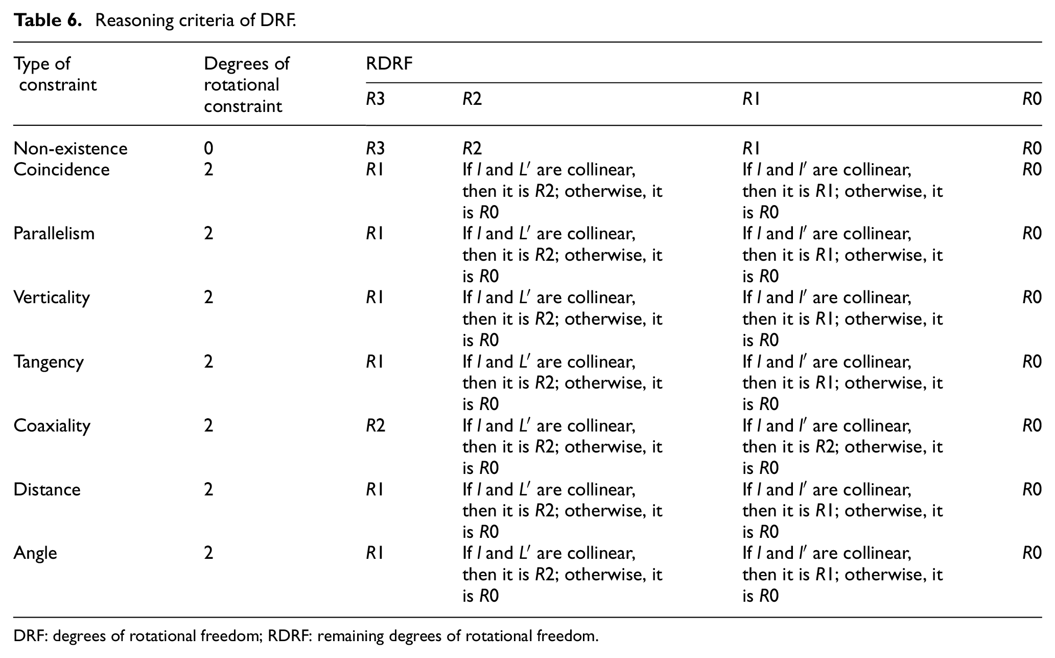
DRF: degrees of rotational freedom; RDRF: remaining degrees of rotational freedom.

Assembly positioning solving based on geometric constraints

The purpose of assembly positioning solving is to determine the pose of the parts according to the assembly constraints and to update their remaining DOF and the RFS. In the unconstrained state, the part is completely free and its pose in space is unlimited. In the constrained state, in order to satisfy the constraints, the parts of the space inevitably change in pose and the ultimate result is that the RFS is limited. The part’s movement can be decomposed into rotational movement and translational movement. Then, the geometric constraints on the part can also be expressed as limitations on the rotational movement and translational movement, that is, the DRF, DTF, rotational FS and translational FS of the part are restricted. The restricted space is removed from the part’s current RFS, and the RFS after applying the constraint is obtained.

The process of assembly positioning is as follows. First, the RFS of the part is obtained through the analysis and DOF determination of the part. Then, the pose transformation matrix is solved in the RFS according to the geometric constraints, including the rotational transformation matrix M_R and the translational transformation matrix M_T. The new geometric constraints of the part are satisfied through pose transformation, and the DOF information of the part is updated to prepare for the next constraint solving.

If the geometric constraints meet the feasibility requirements, the pose transformation matrix M can be expressed as $M = M_{R} \cdot M_{T}$ .

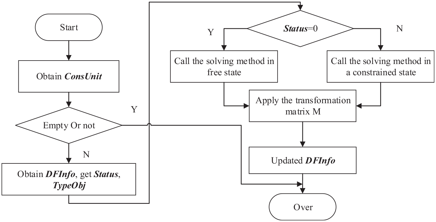
The process of assembly positioning solving is shown in Figure 6, and the specific steps are as follows:

Step 1: Through the interactive constraint definition module, get the newly imposed geometric constraint ConsUnit. If ConsUnit is empty, go to Step 6.

Step 2: Get the DOF information DFInfo from the part to be assembled, get the DOF status Status from DFInfo, get the type of DOF (Type), get the object of DOF (TypeObj), which are the mathematical parameters that describe the RFS.

Step 3: If Status = 0, the part to be assembled is completely free and ‘assembly and positioning method in a completely free state’ is invoked to determine the assembly relationship. If Status = 1, it is in a state of constraint and the ‘assembly and positioning method in the constraint state’ is invoked to determine the assembly relationship.

Step 4: Solve and obtain the pose transformation matrix M, apply M to the part to be installed and determine its correct position and orientation.

Step 5: Update the DFInfo of the part to be installed.

Step 6: Positioning end.

When performing positioning solving of components, there are mainly two kinds of situations. One is an unconstrained state where the assembly positioning solving is in a completely free state. The other kind is assembly positioning solving in the constrained state.

Figure 6.

The process of assembly positioning solving.

Completely free state

The previous section shows that geometric constraint positioning solving can be divided into two steps: (1) orientation solving, that is, rotational transformation matrix solving; and (2) positioning solving, that is, translational transformation matrix solving.

In the free state, the specific steps are as follows:

Step 1: According to ConsUnit, obtain the list of geometric elements that participate in the constraint GeomElemList. According to the parameter information of two geometric elements, determine the rotation axis $L_{axis}$ and the angle $α$ .

Step 2: According to ConsUnit, obtain the type of constraint and determine the rotation angle $θ$ .

Step 3: Solve the rotational transformation matrix M_R. Under the action of M_R, the direction of the geometric elements involved in the constraint satisfies the constraint requirements.

Step 4: Based on the rotational transformation, solve the translational transformation matrix M_T. Under the action of M_T, the position of the geometric elements involved in the constraint satisfies the constraint requirements.

Step 5: According to M_R and M_T, determine the pose transformation matrix M of the parts to be installed.

The following section takes the coaxiality constraints of a cylindrical surface as an example. Constraint positioning solving is analysed in the free state. As shown in Figure 7, there are two parts in space: part A is the part to be mounted and part B is the reference part.

Figure 7.

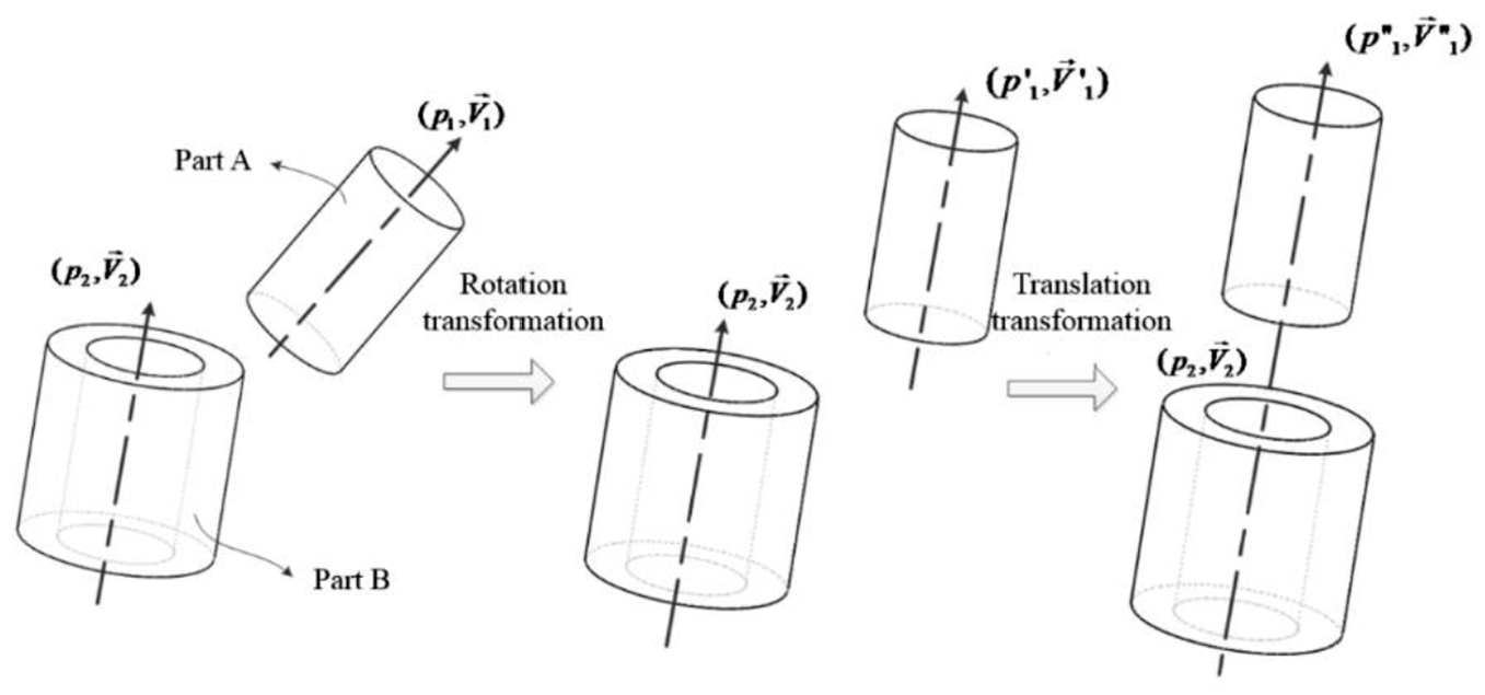
The process of coaxiality constraint positioning.

In the figure, ${\vec{V}}_{1}$ is the direction vector of the cylinder axis of part A and $P_{1}$ is a point on the cylinder axis of part A, where $P_{1} = (x_{1}, y_{1}, z_{1})$ . ${\vec{V}}_{2}$ is the direction vector of the cylinder axis of part B, and $P_{2}$ is a point in the cylinder axis of part B, where $P_{2} = (x_{2}, y_{2}, z_{2})$ .

1. Orientation solving

Positioning and orientation solving are required to calculate the rotational transformation matrix, so the cylindrical surfaces of parts A and B are parallel.

We first calculate the rotational transformation matrix to determine the rotational axis and rotation angle. Assuming that the rotational axis is L, $L = (\vec{e}, P)$ , where $\vec{e}$ represents the direction vector of the rotational axis; P is a point on the axis, where P = (x_p, y_p, z_p). The rotation angle is $θ$ . According to the direction vectors ${\vec{V}}_{1}$ and ${\vec{V}}_{2}$ of the cylinder axis of parts A and B, we calculate the direction vector of the rotation axis, $\vec{e} = {\vec{V}}_{1} \times {\vec{V}}_{2}$ . The rotation angle $θ = \arccos \frac{| {\vec{V}}_{1} \cdot {\vec{V}}_{2} |}{| {\vec{V}}_{1} | | {\vec{V}}_{2} |}$ . Then the rotational transformation matrix M_R of the part can be calculated.

2. Positioning solving

The positioning solution is to calculate the translational transformation matrix on the basis of orientation solving, making the cylinder axes of parts A and B coincide.

Assuming that the translational vector is $\vec{t} = (x_{t}, y_{t}, z_{t})$ , we make $| \vec{t} |$ be the minimum, so $(x_{t}, y_{t}, z_{t}) = (P_{2} - P_{1}) - [(P_{2} - P_{1}) \cdot {\vec{V}}_{2}] \cdot {\vec{V}}_{2}$ . The translational transformation matrix is calculated as M_T.

Therefore, to summarise positioning and orientation solving, the pose transformation matrix of part A is $M = M_{R} M_{T}$ .

Constrained state

When the component to be installed is in a constrained state, the pose transformation matrix needs to be solved in the RFS of the component to achieve its assembly positioning.

In the constrained state, the specific steps are as follows:

Step 1: Get DOF information DFInfo from the part to be assembled, get the type of DOF (Type), get the object of DOF (TypeObj), that is, the RFS.

Step 2: According to ConsUnit, obtain a list of geometric elements that participate in the constraint GeomElemList. According to the parameter information of the two geometric elements, determine the rotational axis $L_{axis}$ and the angle $α$ .

Step 3: According to ConsUnit, obtain the type of constraint. Under RFS, determine the rotation angle.

Step 4: Solve the rotational transformation matrix M_R. Under the action of M_R, the direction of the geometric elements involved in the constraint satisfies the constraint requirements.

Step 5: Based on the rotational transformation, solve the translational transformation matrix, M_T. Under the action of M_T, the positioning of the geometric elements involved in the constraint satisfies the constraint requirements.

Step 6: According to M_R and M_T, determine the pose transformation matrix M of the parts to be installed.

The following section takes the constraints of surface–surface coincidence and surface–surface verticality as an example. The constraint positioning is analysed in the constrained state. As shown in Figure 8, there are two parts, A and B, in space. Part A is the part to be mounted, and part B is the reference part.

Figure 8.

The positioning process of the verticality constraint under a coincidence constraint.

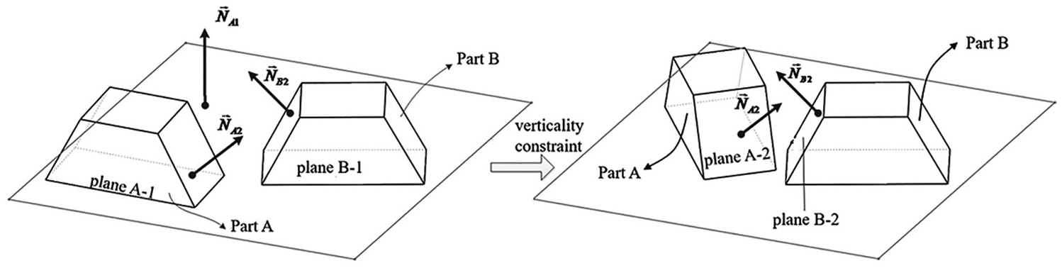
In the free state, the constraints of surface–surface coincidence (between planes A-1 and B-1) are applied on part A (to be mounted) and the reference part B. According to the free-state assembly and positioning solving method, we achieve coincidence between planes B-1 and A-1. At this time, the rest of part A (to be mounted) includes the degree of rotational freedom which is the normal vector $\vec{N} A 1$ winding plane A-1 and the degree of translational freedom along plane A-1. On this basis, the constraints of surface–surface verticality (plane A-2 and plane B-2) are applied on the reference part and the part to be mounted. The verticality constraint only has an angular relationship and does not have a positional relationship.

Under the coincidence constraint, the positioning solving of the verticality constraint is shown in Figure 9. The specific analysis process is as follows.

Supposing the unit normal vectors of planes A-2 and B-2 are $\vec{N} A 2$ and $\vec{N} B 2$ , respectively. Normal vector $\vec{N} A 2$ rotates 360 degrees around $\vec{N} A 1$ to form a conical surface C-1 with a vertex P_c. Suppose a plane $B' - 2$ which passes P_c and is parallel to B-2.

When the plane $B' - 2$ intersects the conical surface C-1, as shown in Figure 9(a), the direction vector of the line intersecting plane $B' - 2$ and the conic plane C-1 is $\vec{V} = {\vec{V} i | i = 1, 2, 3, 4}$ . Suppose that the projection of $\vec{N} A 2$ is $\vec{N} AP 2$ on plane A-1 and the projection of $\vec{V}$ on plane A-1 is $\vec{V} P$ , so the angle between $\vec{N} AP 2$ and $\vec{V} P$ is the rotation angle θ. The rotational axis is $\vec{N} A 1$ , that is, part A (to be mounted) rotates about θ around $\vec{N} A 1$ to obtain a rotational transformation matrix, such that plane A-2 is perpendicular to plane B-2. Therefore, adding face-to-face verticality constraints is feasible.

When plane $B' - 2$ is tangential to conical surface C-1, as shown in Figure 9(b), the direction vector of the line intersecting plane $B' - 2$ and conic plane C-1 is $\vec{V} = {\vec{V} i | i = 1, 2}$ . Suppose that the projection of $\vec{N} A 2$ is $\vec{N} AP 2$ on plane A-1, and the projection of $\vec{V}$ is $\vec{V} P$ on plane A-1, so the angle between $\vec{N} AP 2$ and $\vec{V} P$ is the rotation angle θ. The rotational axis is $\vec{N} A 1$ , that is, the part to be mounted (A) rotates about θ around $\vec{N} A 1$ to obtain a rotational transformation matrix such that plane A-2 is perpendicular to plane B-2. Therefore, adding face-to-face verticality constraints is feasible.

When plane $B' - 2$ and conical surface C-1 do not intersect, applying constraints of surface-to-surface coincidence, which is plane A-2 and plane B-2 with face-to-face verticality constraints, is not feasible.

Figure 9.

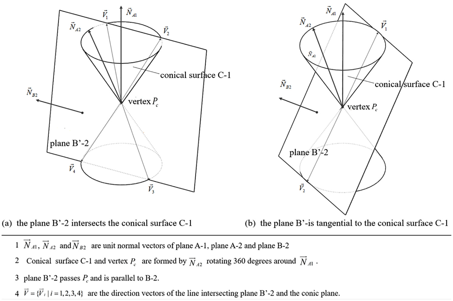
Schematic diagram of positioning solving of the verticality constraint under the coincidence constraint.

System application verification

Module development and implementation process

Based on the software modules of ACIS and HOOPS, a prototype computer-aided process planning (CAPP) system was developed in our laboratory. The proposed method was implemented as a module for fixture management and fixture operation. By using this module, many tools have been managed and applied successfully. To demonstrate the basic point of this article, the process of fixture operations management was tested.

Fixture module

Fixture involves a variety of devices, which ensure that the assembly process can be properly implemented. These devices include fixtures, knives, measuring tools, auxiliary tools and inspection tools. This article focuses on assembly fixtures, which provide reliable positioning by applying external forces to the reference component. This facilitates the assembly of the components and improves assembly accuracy, efficiency and safety.

As shown in Figure 10, in fixture management, tooling extension, tooling deletion, tooling preview and tooling import are implemented. In the tooling application, ‘tooling modelling’, ‘tooling movement’, ‘tooling assembly’ and ‘tooling exit’ can be achieved. Of these, the most critical are tooling modelling and tooling assembly. The fixture is imported to build the fixture model. Then, the assembly of the fixture can be achieved by determining the relationship between the assembly constraints and positioning.

Figure 10.

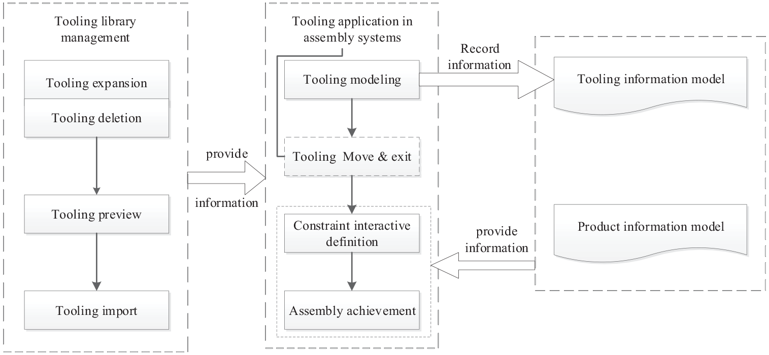
Fixture management and application.

Assembly positioning module

In the fixture module, assembly constraints are mainly achieved through four sub-modules: the fixture model, constraint definition, constraint and positioning solving module and constraint management module. The relationship between the modules and data flow is shown in Figure 11.

Figure 11.

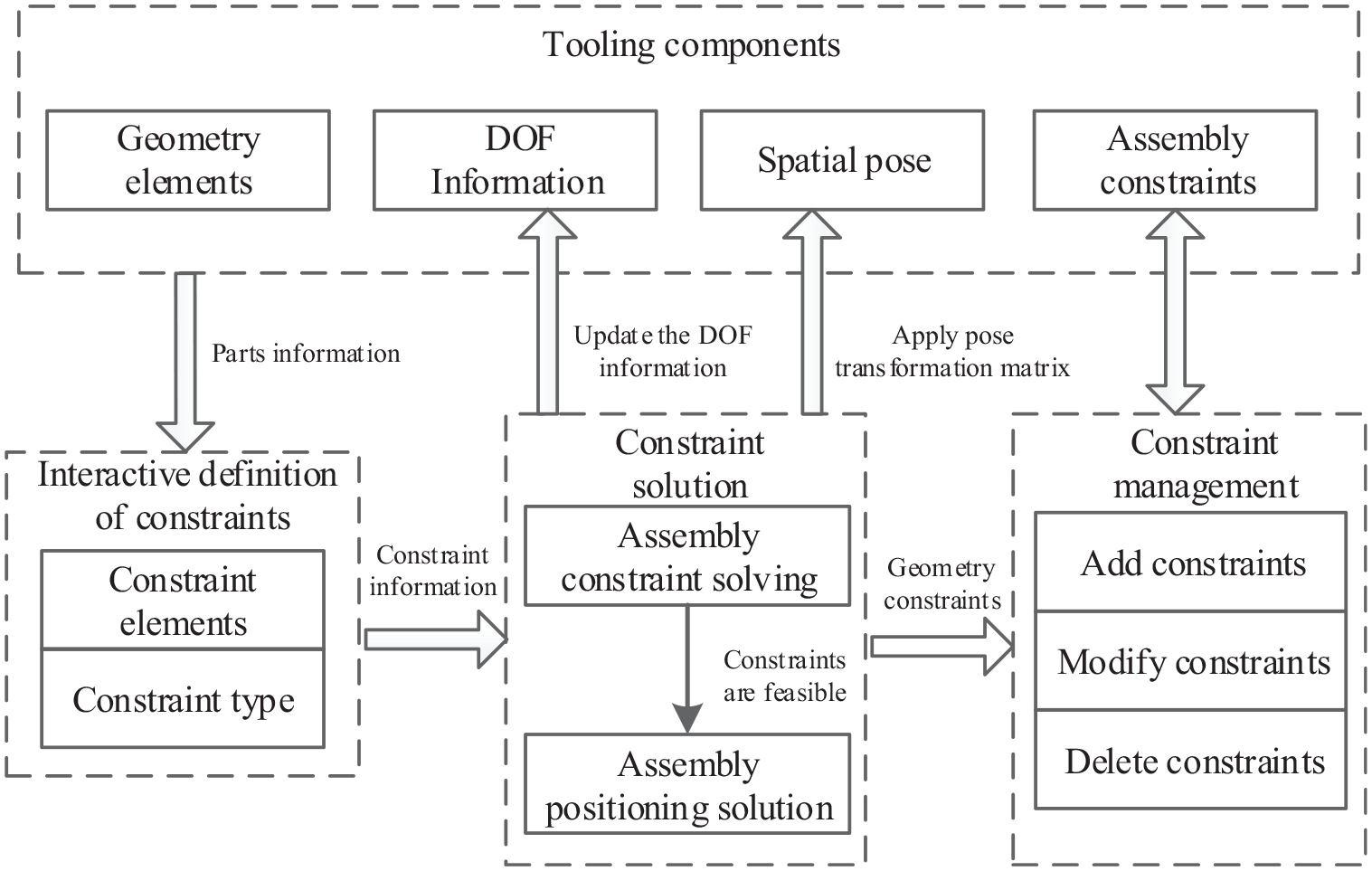
Relationship between sub-modules and data flow.

In the figure, the fixture model represents the component information model, which is the carrier of assembly constraints, including the 3D model information, spatial pose, assembly constraints and DOF information.

The constraint definition module provides an interactive method for defining geometric constraints. The definition process includes the selection of the constrained geometry elements and the constraint relationship types.

The roles of the constraints and positioning solving module are mainly as follows. According to the newly imposed geometric constraints and the current DOF state of components, we can adopt the relevant algorithms to determine the feasibility of the constraint, calculate the spatial pose transformation matrix of the component, adjust the spatial pose of the component and update the DOF information of the component.

The constraint management module manages all feasible geometric constraints and excludes contradictory and redundant ones. The constraint management module’s role is mainly to add, delete and modify geometric constraints and other operations and to interact with the fixture model of constraint information.

The process of implementing assembly positioning

The assembly of components proceeds according to changes in the positions of the components to be mounted relative to the reference component. The component to be assembled is a component that has not been assembled yet, and the reference component is an already-assembled component. Through the constraint relationship between the geometric elements of the components, the pose transformation matrix of the part to be mounted is solved (although a solution may not exist), thereby changing the spatial pose of the components to be mounted to satisfy the assembly relationship between components. The process of interactively adding constraints and implementing the assembly relationship is shown in Figure 12, and the specific steps for its implementation are as follows:

Step 1: Preview the fixture from the fixture library, select the fixture needed and import it into the system.

Step 2: Select the elements that need to have constraints imposed, which are geometric elements.

Step 3: According to the type of geometric element, display the available constraint types and then select the type of constraint to be added (such as coincidence and coaxiality).

Step 4: Solve the geometric constraints and then determine whether the newly imposed constraint conflicts with the component’s current state of constraint, that is, whether the newly imposed constraint is over-constraint.

Step 5: If there is no over-constraint, conduct assembly positioning solving and calculate the pose transformation matrix; otherwise, prompt over-constraint.

Step 6: According to the pose transformation matrix, transform the pose of the part to be assembled according to the constraint state and then update the DOF information.

Figure 12.

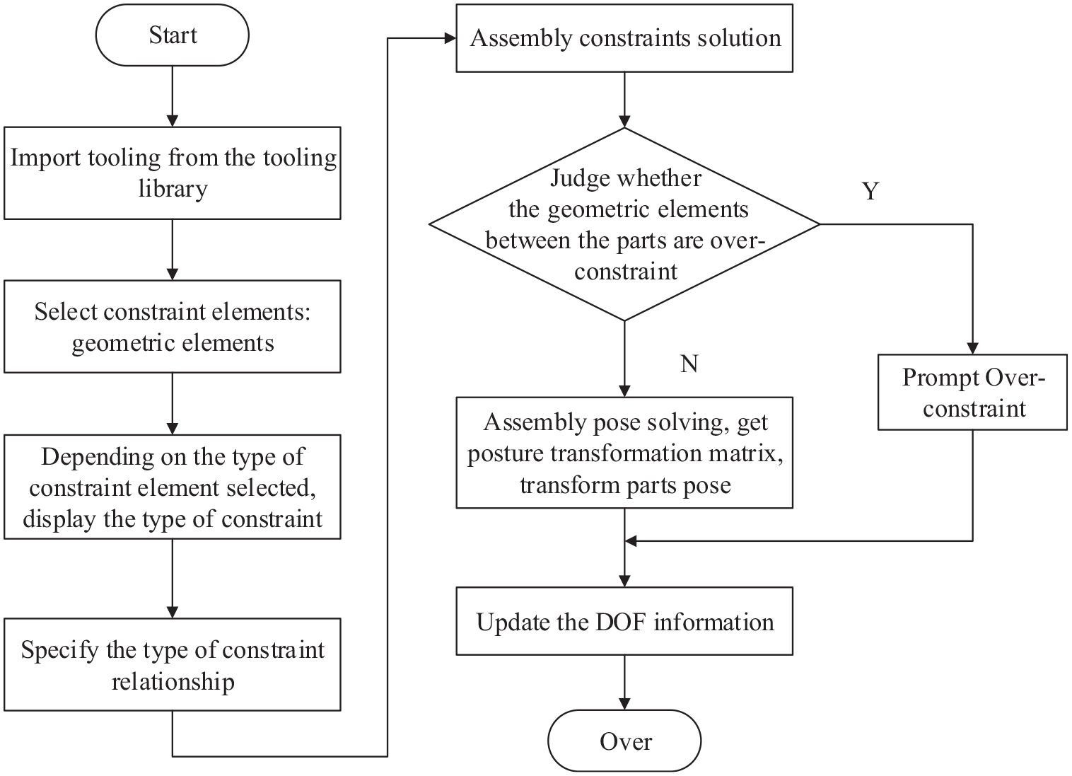
The process of interactively implementing an assembly relationship.

Examples

This article investigated a fixture module for an assembly process planning system based on 3D models. Part of a spacecraft was used as an example to demonstrate the realisation of fixture management, fixture modelling, fixture and product assembly, and generation and application of the assembly process and other functions.

Fixture management

Fixture management involves using the database to classify and manage fixture. Classified by the usage scope, fixture can include common fixtures, special fixtures and standard fixtures. Classified by function, jigs includes cutting tools, measuring tools, jigs and so on. Fixture extension, deletion, preview and import functions in the system were achieved.

1. Extension and deletion of fixture

When there is no suitable fixture in the fixture library, the system supports the importation of external fixture data. As shown in Figure 13, the ‘file open’ window is called to open the fixture. Then, according to the need, the fixture and corresponding categories to be added can be chosen, and the fixture is added to the tool library, as shown in Figure 14.

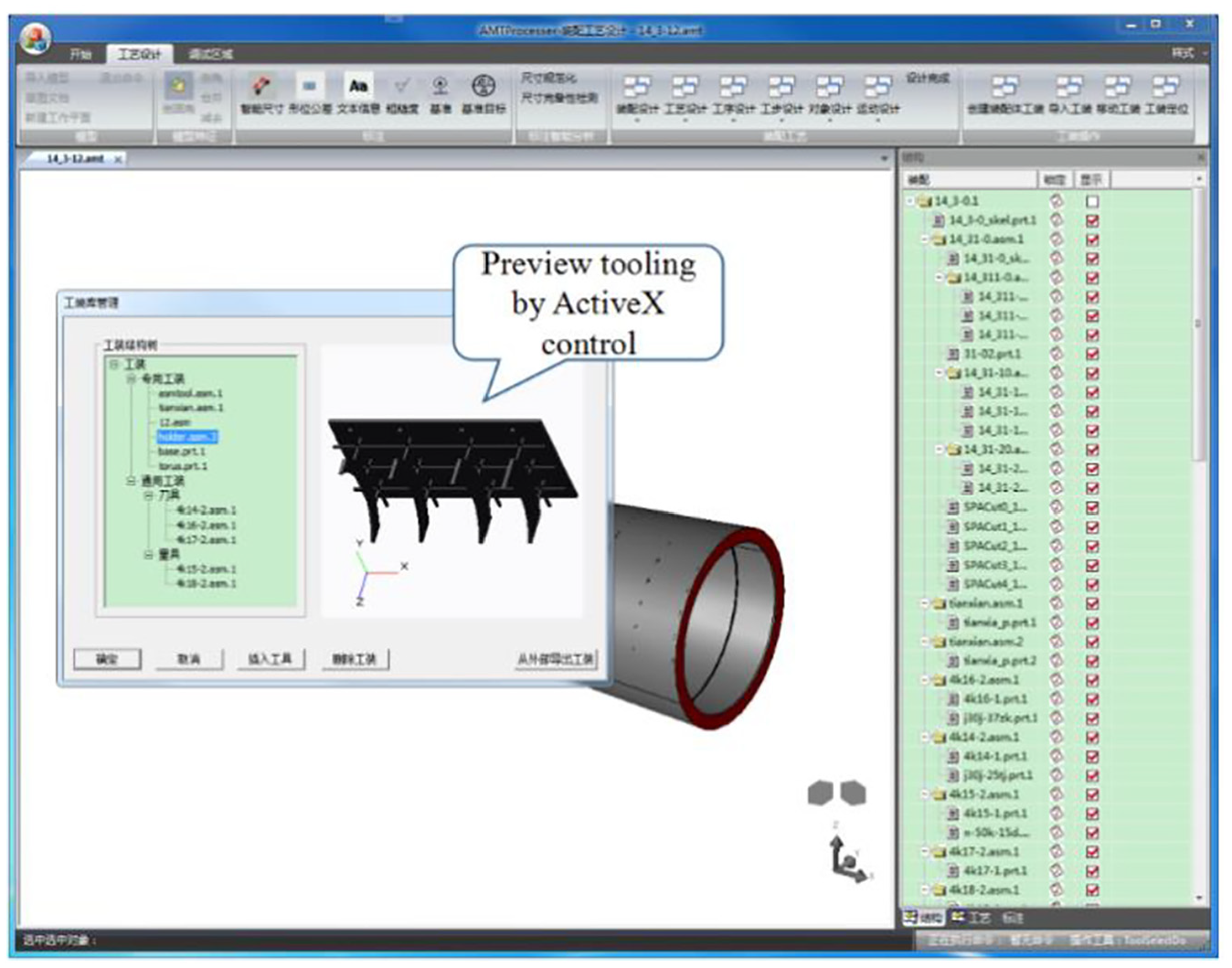
When you need to delete a tooling set from the fixture library, as shown in Figure 15, select the tooling in the fixture management tree and click the ‘Delete’ button. Before importing a selected tooling set into the system, preview it with the ActiveX control to get the correct one, as shown in Figure 16.

2. Importing fixture

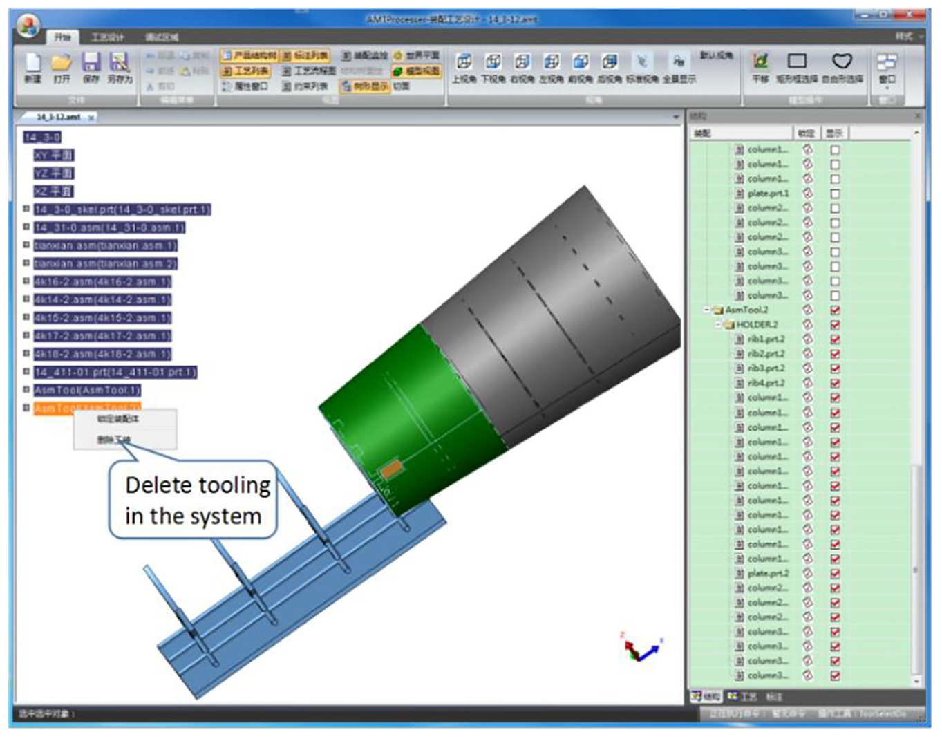
The imported fixture files can be for part tooling or fixture. Commercial CAD fixture files (e.g. Pro/E files) can be opened in the system. After the fixture file is imported, the fixture model is built in the system and the fixture 3D model is displayed in the model view area, making the fixture compatible with the 3D model of the product. Meanwhile, the fixture structure is displayed in the Structure View, which can display or hide fixture components. In addition, fixture can also be moved and removed. Removing the fixture is done, as shown in Figure 17.

Figure 13.

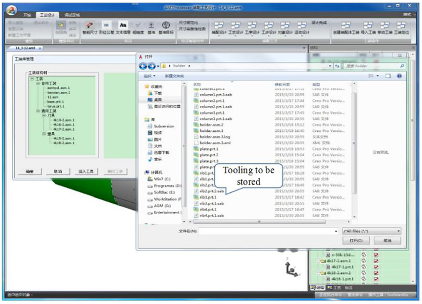
Import of tooling from outside the tooling library.

Figure 14.

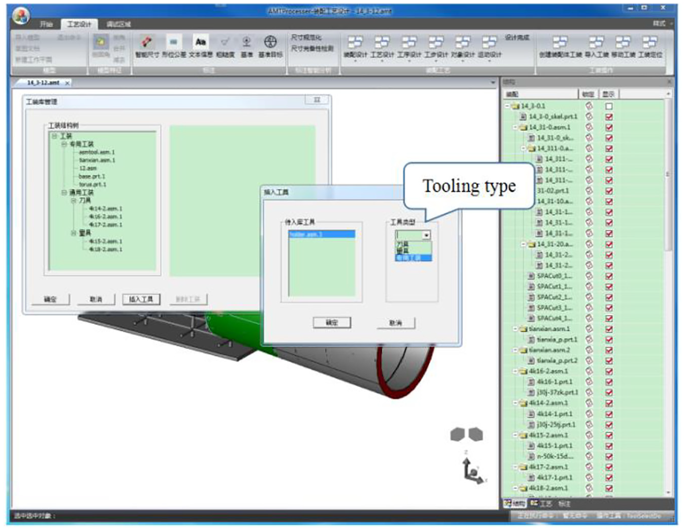
Fixture library extension.

Figure 15.

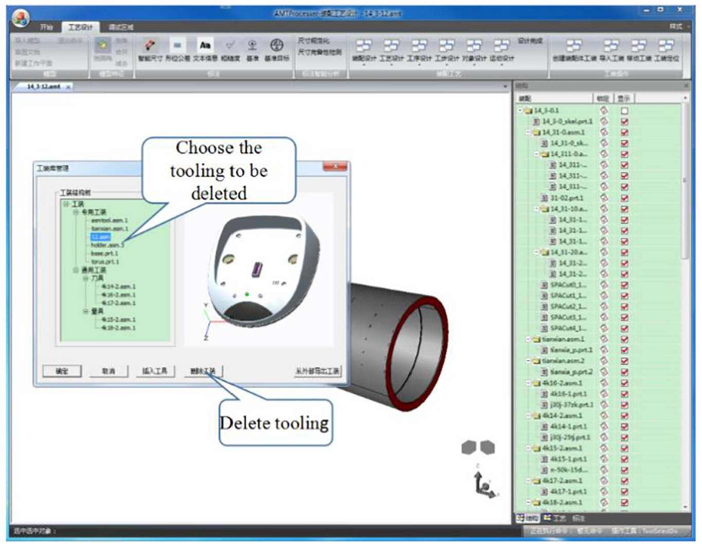
Fixture deletion.

Figure 16.

Fixture preview.

Figure 17.

System fixture deletion.

Operation of fixture assembly

In the system, the general process of fixture assembly is as follows: (1) ‘create the fixture’ as the fixture of the current activity, (2) import the fixture components, (3) assemble the fixture and (4) after the assembly of the fixture is completed, the fixture acts as the fixture of the current activity and completes the assembly operation with the product.

1. Assembly of fixtures

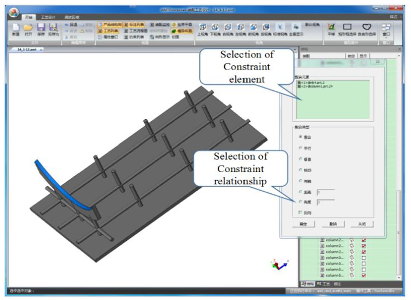
As shown in Figure 18, first, the user selects the geometric surface of the fixture component as the constraint element. The benchmark component is the part which the first selected geometric surface belongs to,Select the component which the geometric surface belongs to after assembly. Then, the user selects the type of constraint relationship. The geometric surface type and the constraint type should match; otherwise, the constraint type is not applicable. Finally, if the constraint relationship is feasible, assembly positioning is achieved and a reverse constraint can also be imposed. Multiple geometric constraints on two parts are used to achieve their assembly.

2. Fixture and product assembly

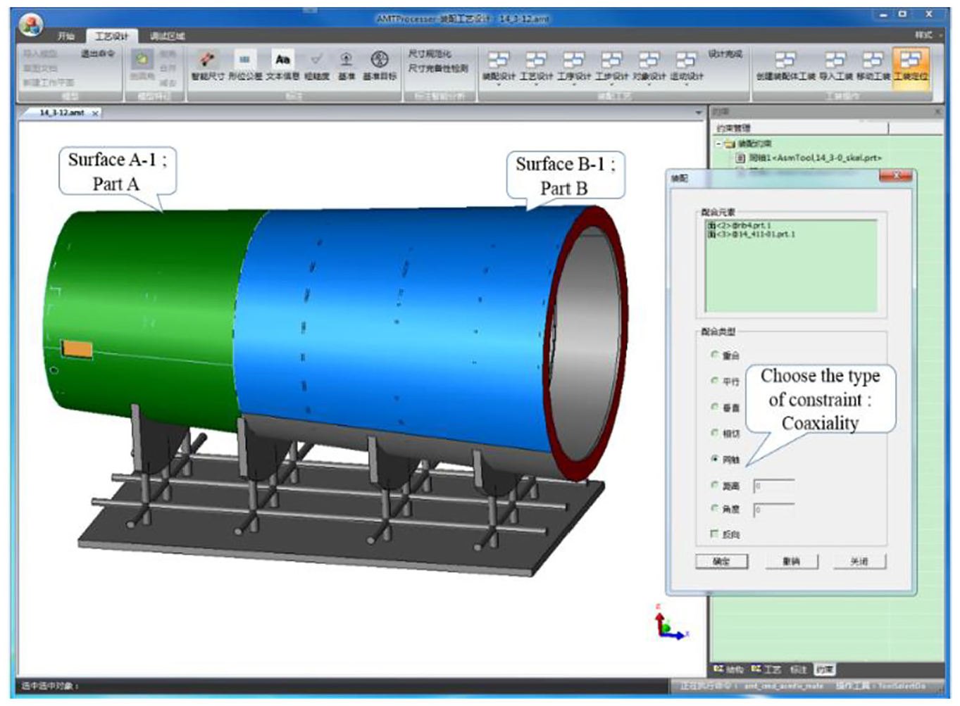
The assembly of fixture and products is similar to the process of fixture part assembly. The only difference is that the product is a benchmark, while the fixture is a to-be-installed part. As shown in Figure 19, a coincidence constraint is completed between the affixing surfaces of the tooling part and the product part. The following shows the specific positioning solution process of coaxiality constraint of fixture parts and product parts.

Step 1: Through the interactive constraint definition module, the newly imposed geometric constraint ConsUnit is obtained. Then, ID_C is obtained and the constraint type is obtained, which is coaxiality. The two geometric elements that participate in the constraint are obtained, which these elements are Surface A-1 and Surface B-1. The two-part geometry models corresponding to GeomElemList are obtained, which are Parts A and B.

Step 2: DOF information DFInfo is obtained from Part B, and the DOF status is obtained from DFInfo, Status = 1. According to the DOF reasoning, Part B is subjected to a coincidence constraint, and the DC is R2. Thus, the type of DOF obtained is R1. According to the shape and position expressions of FS (see ‘Shape and position expression of FS’ section), the object of DOF TypeObj is obtained, which is the mathematical parameter that describes the RFS.

Step 3: If Status = 1, it is in a state of constraint, and the assembly and positioning method in the constrained state is invoked to determine the assembly relationship.

Step 4: The pose transformation matrix M is solved and obtained, matrix M is applied to the part to be installed and its correct position and orientation can then be determined.

Step 5: The DFInfo of the part to be installed is updated.

Step 6: Positioning is over.

In the constrained state, the specific steps are as follows:

Step 1: DOF information DFInfo is obtained from Part B. The type of DOF obtained is R1, and the object of DOF TypeObj is obtained.

Step 2: According to ConsUnit, the list of geometric elements that participate in the constraint GeomElemList is obtained, which are Surface A-1 and Surface B-1. According to the parameter information of the two geometric elements, the rotational axis $L_{axis}$ and angle $α$ are obtained.

Step 3: According to ConsUnit, the type of constraint is obtained, which is coaxiality. Under RFS, the rotation angle θ is obtained.

Step 4: According to the method in the ‘Assembly positioning solving based on geometric constraints’ section, the rotational transformation matrix M_R is solved.

Step 5: Based on the rotational transformation, the translational transformation matrix M_T is solved.

Step 6: According to M_R and M_T, the pose transformation matrix M of the parts to be installed is determined.

Figure 18.

Assembly of fixture parts.

Figure 19.

Fixture and product assembly.

When there is over-constraint, not being assembled is prompted in the system, as shown in Figure 20.

Figure 20.

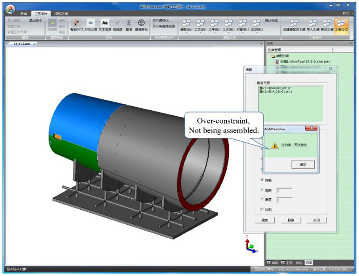
Judgement of over-constraint.

Conclusion and future work

This article studies a fixture information model, methods of solving assembly constraint and assembly positioning. The fixture information model includes fixture management information, display information, geometric information, assembly constraints and DOF information, and related information is defined and expressed by the fixture information model to achieve management and assembly operations. A method of solving assembly constraints based on DOF reasoning is proposed. First, through the analysis of constraints, the relationship between DOF and constraints is determined. Second, mathematical expressions of DOF provide data for DOF reasoning. Finally, the rules for solving DOF reasoning are given. A method of assembly positioning based on geometric constraints is proposed. That is, the rotational transformation matrix and the translational transformation matrix are, respectively, solved according to the newly imposed geometric constraints without breaking the original constraints. This process achieves pose transformation that meets the newly imposed constraint relationship and updates the DOF information. Methods for solving the rotational transformation matrix and the translational transformation matrix in free and constrained states were described.

The work proposes the algorithm and implements them in our assembly process planning prototype system. The algorithm in commercial CAD is a design for assembly, while the algorithm in our system is a design for the assembly process. As a result, differing from commercial CAD, the product assembly undergoes an assembly process in our prototype CAPP system. Through many assembly practices, the assembly speed is at the same level as foreign commercial CAD. At present, we have a qualitative analysis of assembly performance and algorithm performance compared to commercial CAD. For detailed quantitative analysis of performance, more experiments will be performed.

In this article, the assembly constraints and assembly positioning solutions provided are for common geometric surfaces. They do not consider point and line geometry elements; hence, further study is needed to improve assembly positioning. Fixture research is still imperfect, as the assembly and disassembly operating characteristics of fixture and the specific impact of fixture on the assembly process need further study.

Footnotes

Declaration of conflicting interests

The author(s) declared no potential conflicts of interest with respect to the research, authorship, and/or publication of this article.

Funding

The author(s) disclosed receipt of the following financial support for the research, authorship, and/or publication of this article: The authors acknowledge the financial support sponsored by the National Key Research and Development Program of China (grant no. 2018YFB1701301) and the Preliminary Research Program of Equipment Development Department of China (grant no. 61409 230103).

ORCID iD

Xiaojun Liu

References

Boothroyd

. Product design for manufacture and assembly. Comput Aided Des 1994; 26: 505–520.

Ding

Sun

. Multistage rotational optimization using unified Jacobian–Torsor model in aero-engine assembly. Proc IMechE, Part B: J Engineering Manufacture 2017; 233: 251–266.

Fei

. An approach to minimizing surplus parts in selective assembly with genetic algorithm. Proc IMechE, Part B: J Engineering Manufacture 2015; 229(3): 508–520.

Jayaram

Wang

. VADE: a virtual assembly design environment. IEEE Comput Graph Appl 1999; 19: 44–50.

Corrado

Polini

. Assembly design in aeronautic field: from assembly jigs to tolerance Analysis. Proc IMechE, Part B: J Engineering Manufacture 2016; 23: 2652–2663.

Zhang

Liu

. The mapping algorithm for 3D assembly process tree to assembly process flowchart. Manuf Automation 2015; 2: 127–131.

Liu

Yang

. Digital modeling method for 3D assembly process planning model. Trans Beijing Inst Technol 2015; 1: 7–12.

Zhang

Yuan

Zhang

. A new discrete double-population firefly algorithm for assembly sequence planning. Proc IMechE, Part B: J Engineering Manufacture 2016; 361(2): 241–256.

Bourjault

. Contribution to a methodological approach of automated assembly: automatic generation of assembly sequence. Doctoral Dissertation, University of Franche-Comte, Besancon, 1985.

10.

De Fazio

Whitney

. Simplified generation of all mechanical assembly sequences. IEEE J Robot Automat 1987; 3(6): 640–658.

11.

Baldwin

. An integrated computer aid for generating and evaluating assembly sequences for mechanical products. IEEE Trans Robot Automat 1991; 7(1): 78–94.

12.

Gao

. Research on assembly sequence generation and evaluation method in assembly process planning. Comput Integrat Manuf Syst 1998; 2(1): 25–27.

13.

Jiang

Zhang

. Research on automated calculation of assembly direction for feature based assembly process planning. J Tsinghua Univ Nat Sci 1998; 38(11): 45–47.

14.

Homem de Mello

Sanderson

. A correct and complete algorithm for the generation of mechanical assembly sequence. IEEE Trans Robot Automat 1991; 7(2): 626–633.

15.

Gottipolu

Ghosh

. Representation and selection of assembly sequences in computer-aided assembly process planning. Int J Prod Res 1997; 35(12): 3447–3465.

16.

Raju Bahubalendruni

MVA

Biswal

. An efficient stable subassembly identification method towards assembly sequence generation. Nat Acad Sci Lett 2018; 41: 375–378.

17.

Raju Bahubalendruni

MVA

Biswal

. A review on assembly sequence generation and its automation. Proc IMechE, Part C: J Mechanical Engineering Science 2016; 230(5): 824–838.

18.

Zhou

Zheng

Yan

, et al. A novel hybrid algorithm for assembly sequence planning combining Bahubalendruni and Biswal 837 bacterial chemotaxis with genetic algorithm. Int J Adv Manuf Technol 2011; 52: 715–724.

19.

Akpinar

Mirac Bayhan

Baykasoglu

. Hybridizing ant colony optimization via genetic algorithm for mixed-model assembly line balancing problem with sequence dependent setup times between tasks. Appl Soft Comput 2013; 13: 574–589.

20.

Hui

Yuan

Kai-fu

. Efficient method of assembly sequence planning based on GAAA and optimizing by assembly path feedback for complex product. Int J Adv Manuf Technol 2009; 42(11–12): 1187–1204.

21.

Sun

Zhang

. Research on assembly sequence dynamic planning method considering resource constraints. Aeronaut Manuf Technol 2014; 8: 36–41.

22.

Yin

Tang

Kang

. Topology face–based change propagation analysis in aircraft-assembly tooling design. Proc IMechE, Part B: J Engineering Manufacture 2014; 230: 120–135.

23.

Phong

Simmy

. A data model for an assembly planning software system. Comp Integr Manuf Sys 1997; 10: 267–275.

24.

Kang

. Research on modeling and simulation technologies of virtual tools for the 3D assembly planning. Master’s Thesis, Huazhong University of Science and Technology, Wuhan, China, 2012.

25.

Hongmin

Fan

. Interactive assembly tool planning based on assembly semantics in virtual environment. Int J Adv Manuf Technol 2010; 51(5–8): 739–755.

26.

Raju Bahubalendruni

MVA

Anil Kumar

Sankar

KMS

. Practically feasible optimal assembly sequence planning with tool accessibility. IOP Conf Ser Mater Sci Eng 2018; 390: 012026.

27.

Cao

Wang

Zhao

. Geometric constraint solving based on niche improved particle swarm optimization. Chinese J Sci Inst 2012; 33: 2125–2129.

28.

Joan-Arinyo

Soto

. A correct rule-based geometric constraint solver. Comp Graph 1997; 21: 599–609.

29.

Qiao

Wang

Xiang

. Solving 3D geometric constraints based on freedom analysis. J Comp Aided Des Comp Graph 2002; 14: 557–561.

30.

Wei

Xiaogang

. The application of improved PSO algorithm in the geometric constraint solving. In: International conference on computer network, Xi’an, China, 23–25 September 2017. New York: IEEE.

31.

Cao

. Solving geometric constraint based on the interactive update mode quantum genetic algorithm. J Image Graph 2016; 21(4): 499–495.

32.

Zhang

Gao

Tan

. Research of movement navigation based on assembly constraint recognition. Chinese J Mech Eng 2002; 15: 6–10.

33.

Liu

, et al. Assembly process modeling mechanism based on the product hierarchy. Int J Adv Manuf Technol 2016; 82: 391–405.

An assembling algorithm for fixture in an assembly process planning system

Abstract

Keywords

Introduction

Literature review

Assembly sequence planning

Information model representation of assembly tooling

Assembly constraint location of assembly tooling

Fixture model in an assembly process system

Expression of the fixture information model

Management information

Display information

Geometric information

Assembly constraints

DOF information

Geometric models and the geometric elements of parts

Assembly constraints and geometric constraints

Expression of the shape and position of fixture geometric elements

Assembly constraint solving and assembly positioning solving

Assembly constraint solving based on DOF inference

Relationship between DOF and constraints

DOF analysis

Shape and position expression of FS

DOF reasoning

DTF reasoning

DRF reasoning

Assembly positioning solving based on geometric constraints

Completely free state

Constrained state

System application verification

Module development and implementation process

Fixture module

Assembly positioning module

The process of implementing assembly positioning

Examples

Fixture management

Operation of fixture assembly

Conclusion and future work

Footnotes

Declaration of conflicting interests

Funding

ORCID iD

References