Sage Journals: Discover world-class research

Abstract

Input uncertainties inevitably result in the output error for parallel mechanisms, which will lead to significant influence on good work performance. To control the output error within the specification boundary, this article proposes a novel approach of input tolerance design based on the level set method for the driving joint. The implementation of the proposed method can be divided into two subtasks. First, using the level set method, the exact input error boundary is determined by means of evolving an initial input error interface with a defined normal speed field, thereby transforming the problem of exploring the exact boundary into solving a partial differential equation with initial value. On this basis, according to the equal and scaled principles, the tolerance width of each input is evaluated in an intuitionally geometrical manner, that is, searching the maximum geometry corresponding to the principle inside the exact input error boundary. Finally, two planar parallel mechanisms with different degrees of freedom are introduced as numerical examples to demonstrate the execution and effectiveness of the proposed method.

Keywords

Parallel mechanism tolerance design input error boundary level set method geometrical manner

Introduction

As practical engineering focuses more and more on precision, accuracy analysis becomes a key issue for the parallel mechanism because a loss will be irreparable if the operation fails owing to the output error.¹ Herein, input uncertainties lead to observable geometric deviations,² which decrease the function and quality of parallel mechanisms, and thus need to be limited by input tolerances. Therefore, it is very necessary to develop an effective and accurate approach to evaluate the maximum tolerance for each actuator.³

In the past, various studies related with tolerance design have been carried out. The most commonly used methods to deal with the tolerance allocation usually involve solving an optimization problem by minimizing production cost subjected to the constraints of the allowable pose accuracy, the manufacturing and assembling feasibilities,⁴ and so on. Building upon statistical or worst-case error models, a series of cost-tolerance functions such as exponential model,⁵ reciprocal model,⁶ and polynomial model⁷ have been proposed, and several algorithms have been developed to improve computational efficiency.^5,8,9 For example, Muthu et al.¹⁰ proposed an optimal tolerance design for assembly based on a non-linear integer model, considering both the manufacturing cost of each component and the assembling quality loss. Krishna and Rao¹¹ used an optimization technique originating from the area of metaheuristics to determine the optimal tolerance to realize the minimum manufacturing cost. Jawahar et al.¹² reported a tolerance allocation model for interchangeable assembly that, in essence, was based on searching the Pareto front of a multi-objective optimization by an iterative algorithm. Ni et al.¹³ implemented the tolerance design by means of sensitivity analysis, in which a genetic algorithm was applied to allocate the manufacturing tolerance of each part. Lin et al.¹⁴ reported a kinematic error analysis and tolerance design of cycloidal gear reducers, where the tolerances were optimized with the objective of minimizing the manufacturing cost.

Besides, mathematical approaches for the representation of geometric tolerances in tolerance simulation models have been proposed, such as vectorial tolerancing,¹⁵ the model of technologically and topologically related surfaces,¹⁶ the direct linearization method,¹⁷ the deviation domain¹⁸ relying on the small displacement torsor,¹⁹ statistical method,²⁰ and tolerance maps.²¹ Such tolerance analysis is useful for designers in understanding and verifying whether the output performance is locating within the specified limits or not.²² In addition, several scholars applied some new methods in tolerance design and analysis. Goldsztejn et al.²³ evaluated the maximal pose error given an upper boundary owing to parameters uncertainties by Kantorovich theorem, and then utilized the approximate linearization to determine the tolerances. Zhang et al.²⁴ proposed a novel tolerance analysis framework incorporating skin model shapes and a classic boundary element method, which aims to consider the interactions between form errors and local surface deformations during assembly simulation and tolerance analysis. Homri et al.²⁵ used a metric modal decomposition to model the form defects of various parts in a mechanism and utilized optimization method to assess the assemblies. Armillotta²⁶ pioneered to treat tolerance analysis as a problem analogous to the force analysis for linkages. Mazur et al.²⁷ reported an application of polynomial chaos expansion in tolerance analysis, by which the uncertainty quantification was described.

Obviously, most researchers paid plenty of attentions to tolerance synthesizing of parts. These models have been mainly used for manufacture or assembly tolerance analysis, that is, analyzing the effects of geometric tolerances on the machinability and assemblability,^28,29 as this has been the main concern in tolerancing for many years.^30,31 Conversely, the focus on how to evaluate the input tolerance for the driving joint to control the output error is comparatively limited. As a matter of fact, the driving process is inherently imprecise, triggering the end-effector deviates from the nominal pose inevitably. To solve this problem, this study proposes a novel approach of input tolerance design for the parallel mechanism to ensure the pose error of the end-effector locates inside the design limitation. Compared to the previous works mainly by means of an optimization or statistical method, there are two major advantages of the proposed method. First, this method can rapidly give the geometric surface of the input error space in the case of a given output accuracy specification. Second, this method lets us deal with the tolerance design from a perspective of geometric insight, which is quite intuitive and provides the physical interpretation for the designer to calculate the input tolerance bands.

The rest of this article is arranged as follows. The “Problem description” section gives a brief description of the studied problem. Then, the “Evaluation of the input error boundary” section demonstrates the evaluation of the input error boundary by means of the level set method. Next, tolerance design according to the exact input error boundary is presented in the “Tolerance design” section. Thereon, two different numerical examples are showcased in the “Numerical examples and discussion” section to illustrate the proposed approach. Finally, conclusions are outlined in the “Conclusion” section.

Problem description

It can be imagined that if the exact input error boundary is obtained, the tolerance band can be determined accordingly. Here, a three-degrees-of-freedom (3-DOF) parallel mechanism is introduced to elaborate this idea. Due to the output accuracy limitation, the practical input error boundary is actually a three-dimensional (3D) surface, denoted as Ω in Figure 1. It is sure that the “error point” inside Ω, whose coordinates represent the input imperfections, satisfies the output accuracy specification. Consequently, the block Ψ formed by the maximum input tolerances (a, b, and c) is certainly locating inside Ω and inscribes the boundary fitly. In other words, if the block Ψ is ascertained in this closed input error boundary, its side lengths, a, b, and c, are just the tolerance bands of the driving joints.

Figure 1.

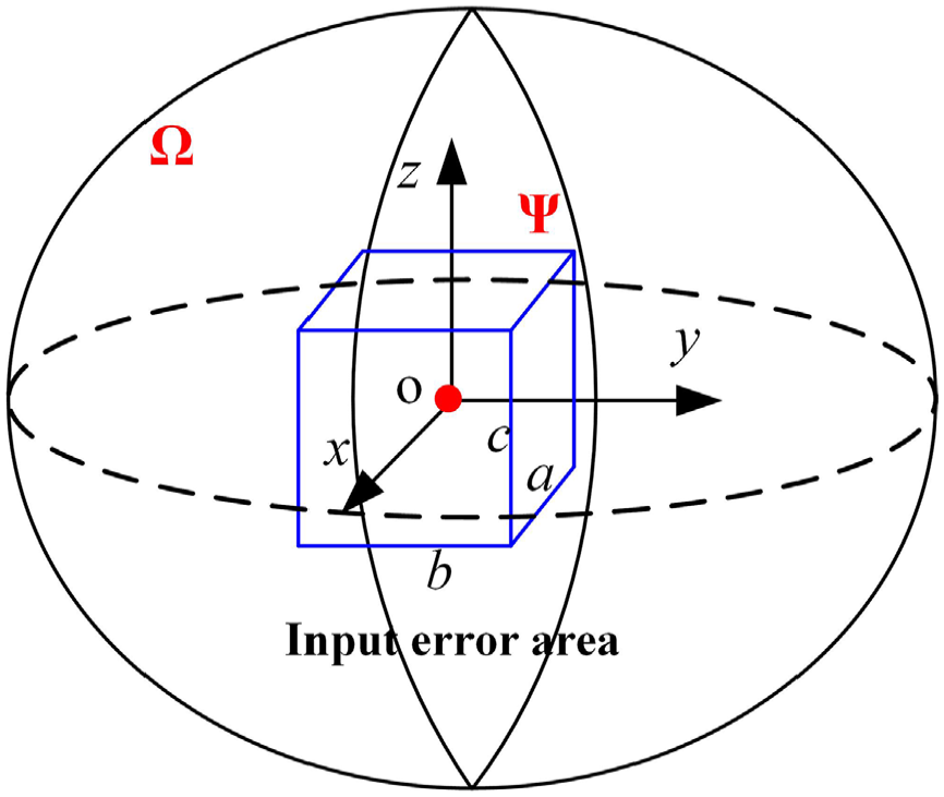
Sketch of input tolerance design using a geometric method.

Therefore, the input tolerance design can be conducted by completing the following two subtasks (the processing deviations of links are not considered in this study):

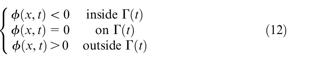
Determining the exact input error boundary Ω subject to the output accuracy specification;

Then searching the corresponding maximum geometry Ψ inside the derived boundary to obtain the tolerance.

Evaluation of the input error boundary

Basic formulation

Accuracy analysis of parallel manipulators can be sorted into two categories: the forward and inverse error boundary analysis.³² In the past, several scholars have put efforts to explore elegant methods to estimate the maximum output error in terms of the input error space.^3,33 Distinguished from them, the inverse error boundary analysis is studied in this article for the input tolerance design.

According to the forward kinematics, there exists a mapping between the input and output error spaces. Therefore, the maximum input error at a given nominal output configuration can be formulated as

\max T = ‖ x - 0 ‖

(1)

which can be constrained by

| δ_{i} - 0 | \leq ε_{i} (i = 1, 2, \dots, m)

(2)

where $x = (x_{1}, x_{2}, \dots, x_{k})$ is a column array collecting the actual input errors and k is the number of the active joints, $δ_{i}$ is the ith element of the pose error $δ$ corresponding to the input error x, $ε_{i}$ represents the accuracy specification of $δ_{i}$ , and m is the component amount of the output pose. Note that the relationship below holds, that is

δ = f (x)

(3)

where f represents the forward kinematics function.

So far, evaluating the maximum input error has been transformed into an optimization problem, in which the input error is selected as the design variables. As a matter of fact, the exact input error boundary is a closed curve (DOF = 2) or 3D surface (DOF = 3) or hypersurface (DOF > 3), and points on them reach the maximum values in arbitrary directions when the output error vector is given. Consequently, the input error boundary can be derived by searching the maximum input error points along all directions.^3,32

Illustration of the level set method

The level set method, a computational technique developed by Osher and Sethian,³⁴ has been a successful tool for simulating a moving interface of co-dimension one because of its simplicity and efficiency. Its successful applications include multi-phase flows,³⁵ the topology optimization of structures,³⁶ the accuracy analysis of parallel mechanisms,³ and image processing.³⁷ Owing to those merits, the level set method is employed here to search the input error boundary.

As depicted in Figure 2, there is a closed interface y = f(x) on the plane denoted by the red line. It can be identified with a higher dimensional function, the time-dependent level set function $φ$ , as

φ (x, y) = y - f (x)

(4)

Figure 2.

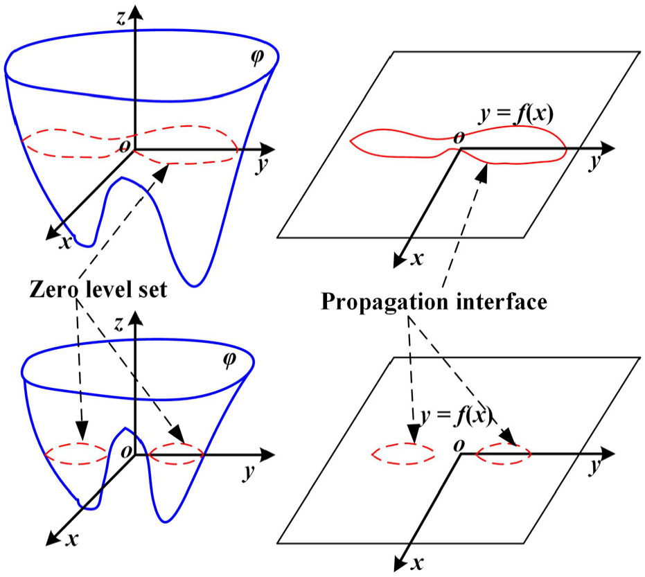
Schematic diagram of the level set propagation.

Accordingly, $φ (x, y) = 0$ is the implicit expression of this curve, expressed as

y (t) = (x | φ (x (t), t) = 0)

(5)

Applying the chain rule to equation (5)³⁸

\frac{\partial φ (x (t), t)}{\partial t} = 0

(6)

φ_{t} + \nabla φ (x (t), t) x_{t} = 0

(7)

where $φ_{t}$ is the partial derivative of the level set function with respect to time, $T_{p_{3}} \nabla φ (x (t), t)$ is the gradient of the level set function, and x_t is the time derivative of the propagating interface.

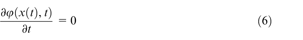
If a curve is propagated, the moving speed

F = x_{t} \cdot n

(8)

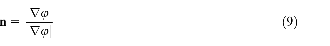
along its normal direction must be given, where n, the normal vector, has a simple representation with $φ$ , given as³⁵

n = \frac{\nabla φ}{| \nabla φ |}

(9)

Thus, equation (7) can be rewritten as

φ_{t} + F | \nabla φ | = 0

(10)

and the initial level set function can be described as

φ_{0} = φ (F (x_{0}, y_{0}), t = 0)

(11)

It is readily seen that equation (10) is just a pure Hamilton–Jacobi equation with a specific normal speed function of the propagating interface and the initial value. Hence, the problem of tracking the input error interface propagation turns out to handle a partial differential equation with the initial value.

Searching the input error boundary

The key of utilizing the level set method to propagate the input error interface lies in two aspects. On one hand, an appropriate “carrier” should be determined to express the interface implicitly, that is, a higher dimension level set function. In general, the distance function is preferred, formulated as³⁸

{\begin{matrix} ϕ (x, t) < 0 & inside Γ (t) \\ ϕ (x, t) = 0 & on Γ (t) \\ ϕ (x, t) > 0 & outside Γ (t) \end{matrix}

(12)

where Γ(t) is the closed moving interface.

On the other hand, the utilization of the level set method depends on the propagation speed. In order to illustrate the definition of the speed function clearly, an imaginary parallel mechanism with two inputs is taken, for example. Suppose that there is an initial input error curve (t = 0; the red dashed line in Figure 3(a)). Through the mapping of the forward kinematics, the corresponding output error curve can be obtained (the red line in Figure 3(b)). Note that the black line in Figure 3(b) encloses the allowable output error area.

Figure 3.

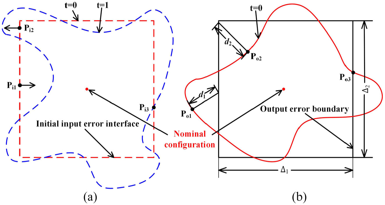
Error interface mapping between the input and output of a planar parallel mechanism: (a) input error interface and (b) output error interface.

From Figure 3(b), it can be seen that some points locate outside the designed output error domain (P_o1), some inside the domain (P_o2), and some exactly standing on the boundary (P_o3). If the point (P_o2) on the output error interface situates inside the allowable space, the corresponding original image (P_i2) on the input error interface, according to the mapping between the work space and joint space, must be one of the points inside the allowable input error area. Otherwise, if the point (P_o1) stands outside the allowable output error scope, the corresponding original one (P_i1) also locates outside the tolerant input error area. Moreover, the original point (P_i3) whose mapping image (P_o3) is on the output error boundary is bound to be one of the points of the exact input error boundary.

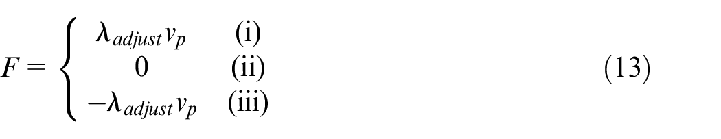
Therefore, to approach the exact input error boundary, the point inside the input error boundary should be pulled out (P_i2); whereas the point outside the input error boundary should be dragged back (P_i1). In addition, the point fitly on the exact input error boundary should not be moved any more (P_i3). In this case, the points on the input error interface can be classified into three categories:^3,39 (i) the point locating inside the exact boundary, (ii) the point just lying on the exact boundary, and (iii) the point situating outside the exact boundary. Based on this classification, the speed function of the propagation front is assigned to be

F = {\begin{matrix} λ_{adjust} v_{p} & (i) \\ 0 & (ii) \\ - λ_{adjust} v_{p} & (iii) \end{matrix}

(13)

where $λ_{adjust}$ is the adjustment coefficient, and

v_{p} = \frac{d_{k}}{σ}

(14)

where $σ$ equals to the sum of all output error intervals—namely, Δ₁ + Δ₂—and d_k denotes the distance of the point on the output error interface relative to the designed boundary along the normal directions such as d₁ and d₂.

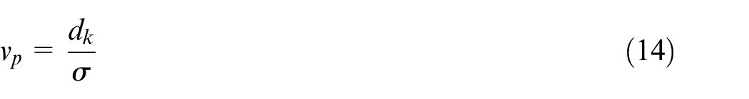
In fact, the ideal case for equation (14) is to use the distance of the point on the input error interface relative to its exact boundary. But because the input error boundary is just our target, this distance cannot be obtained. As a result, the distance of the mapping point on the output error interface relative to the allowable boundary is applied to reflect the closeness degree between the input error propagating front and the target boundary from an indirect perspective. Grounding on equation (14), the speed field of the propagating front can be evaluated, and based on this, a new closed interface (the blue dashed line in Figure 3(a)) can be attained. By repeating the above computation, the exact input error boundary can be obtained until the distance d_k is close enough to zero. Please see more solution details in Sethian and Smereka,³⁵ Peng et al.,³⁸ and Andrew.³⁹

Tolerance design

The tolerance design is exactly to find the maximum interval for the error source so that the corresponding pose deviation of the end-effector locates inside the required domain.¹⁵ The tolerance width is deeply associated with the production cost. If the cost-tolerance function of the actuator is known, the input tolerance design can be conducted by solving the optimization problem at minimizing the cost function, which is constrained by the exact input error boundary. However, the relationship between the tolerance band and production cost of the driving actuator is so complex that there is almost no ready-made cost-tolerance model. Therefore, the principles generally applied in the real-life engineering for tolerance design, namely, the equal and scaled tolerances,^40,41 will be adopted to conduct the input tolerance design for parallel mechanisms. To be specific, the equal tolerance means to select the actuators with the same allowable deviation intervals, whereas the scaled tolerance indicates these intervals are proportional with the prescribed coefficient. In essence, these two principles originate from the linear cost-tolerance model.⁴² In addition, considering the driving actuator usually has the identical possibility of generating deviations along the forward and backward directions, the tolerance band of each input is defaulted to be symmetrical.

Once the tolerance band of each driving joint is determined, the input error “geometry” inside the allowable boundary can be settled down accordingly. Thus, the input tolerance design based on the derived error boundary is essentially to find the maximum equal-side or scaled-side plane/3D/hypergeometry within it. Here, an imaginary 2-DOF parallel mechanism is used, for example.

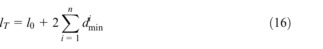
As shown in Figure 4, the input error boundary for a 2-DOF parallel mechanism is actually a closed plane curve. According to the aforementioned principles, the tolerance evaluation for its two actuators can be regarded as finding a maximum square (equal tolerance) or rectangle (scaled tolerance) within the input error boundary. It is worth mentioning that because the tolerance band is symmetrical, the geometrical center of the square or rectangle coincides with the origin of the nominal configuration.

Figure 4.

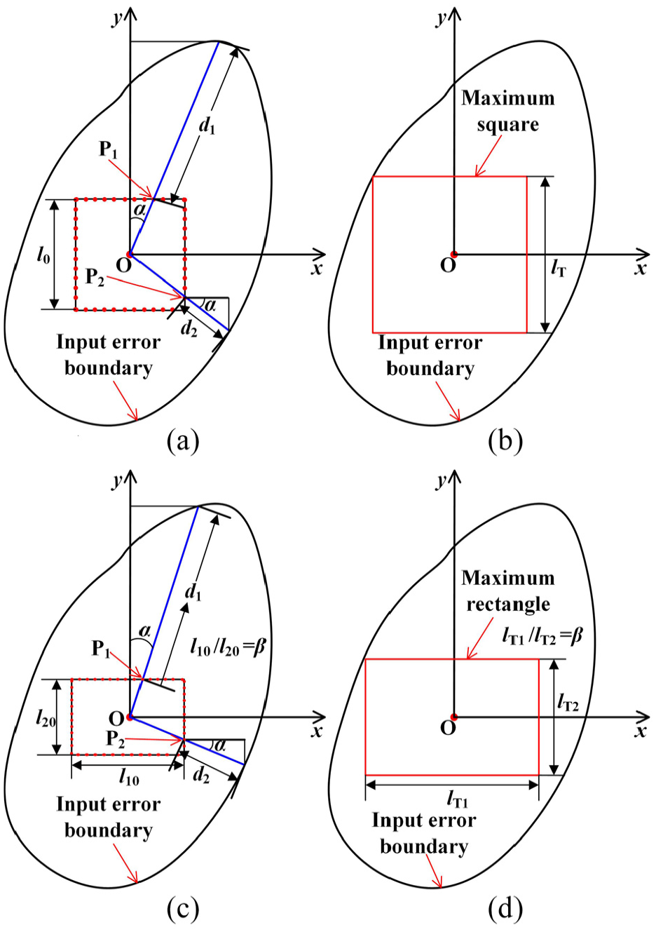
Input tolerance evaluation for a 2-DOF parallel mechanism: (a) initial square, (b) maximum square, (c) initial rectangle, and (d) maximum rectangle.

Equal tolerance

First, a square with a rather small side length is drawn, as shown in Figure 4(a). Then, whether points on this square situate inside the error boundary should be checked. In this case, the four sides are discretized and the distance of each point relative to the error boundary is computed. Suppose that the initial square side length is l₀, and then by sweeping the square, the distance of each point relative to the boundary along the vector direction linking the origin O to itself can be obtained. For example, the distances of P₁ and P₂ relative to the exact input error boundary are d₁ and d₂, respectively. On this basis, project these distances onto the axes, and the minimum distance of the point relative to the error boundary along the axis can be derived, which is denoted as d_min. It is worthy pointing out that if the original distance belongs to the point on the side parallel to x-axis, it should be projected to y-axis; otherwise, project it to x-axis. For instance, the distance of P₂ relative to the boundary along x-axis equals to d₂·cosα₂.

By computing d_min, the closeness degree of the geometry with respect to the exact input error boundary can be assessed. As a result, the initial tolerance square can be extended, and the side length becomes

l_{t} = l_{0} + 2 d_{\min}

(15)

When the new side length l_t is calculated, a new square will be also determined. Subsequently, the same work of computing the minimum distance d_min of the whole points on the square sides should be carried out. By repeating the above operation until the minimum distance d_min vanishes or extremely approaches to zero, the final biggest square can be harvested, as shown in Figure 4(b). At this moment, the side lengths are just the input tolerance bands of the two driving actuators, which can be expressed as

l_{T} = l_{0} + 2 \sum_{i = 1}^{n} d_{\min}^{i}

(16)

where $d_{\min}^{i}$ is the minimum distance d_min of the point on the ith square, and n is the total amount of the squares.

Scaled tolerance

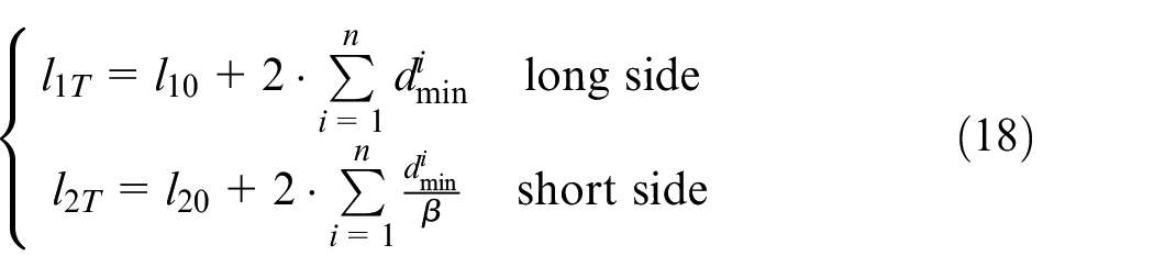
For the scaled principle, an initial small rectangle whose side lengths conform to the prescribed proportionality coefficient is also needed to be assigned inside the allowable input error boundary, as presented in Figure 4(c). Then, similar to the process shown in Figure 4(a), the distances of all points on the sides such as d₁ and d₂ should be computed first to determine d_min. Then, assume that the proportionality coefficient of the tolerance bands of the two inputs is β (β > 1) and extend the initial rectangle. But different from the one shown in Figure 4(a), the side lengths should be evaluated, respectively, and expressed as

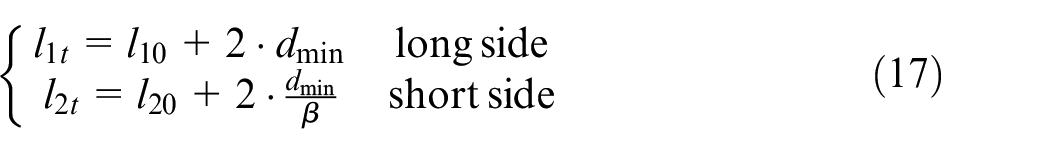
{\begin{matrix} l_{1 t} = l_{10} + 2 \cdot d_{\min} & long side \\ l_{2 t} = l_{20} + 2 \cdot \frac{d_{\min}}{β} & short side \end{matrix}

(17)

Obviously, when l_1t and l_2t are known, the initial rectangle can be updated accordingly. Like the equal principle, repeat calculating d_min and then update the side lengths of the rectangle by equation (17) until the biggest rectangle within the allowable input error boundary is sought, as shown in Figure 4(d). Consequently, the final tolerance width for each actuator can be given as follows

{\begin{matrix} l_{1 T} = l_{10} + 2 \cdot \sum_{i = 1}^{n} d_{\min}^{i} & long side \\ l_{2 T} = l_{20} + 2 \cdot \sum_{i = 1}^{n} \frac{d_{\min}^{i}}{β} & short side \end{matrix}

(18)

It can be readily observed from Figure 4 that the input tolerance design is actually to find the maximum geometry within the exact error boundary, and the side length is just the tolerance width of each driving actuator. Here, a 3-DOF parallel mechanism is considered as another example to illustrate the approach. First, suppose the exact input error boundary has been derived. There is no doubt that this boundary is a 3D surface, as shown in Figure 5. The input tolerance design of the 3-DOF parallel mechanism is to search the maximum cube inside the exact error boundary. Figure 5(a) and (b) gives the schematic diagram of tolerance evaluation for the three inputs according to different principles. Moreover, if the DOF of the parallel mechanism increases, the same operation described above can be generalized directly.

Figure 5.

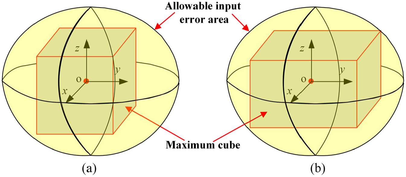
Schematic diagram of tolerance evaluation for a 3-DOF parallel mechanism: (a) equal principle and (b) scaled principle.

Numerical examples and discussion

To demonstrate the effectiveness and generalization of this approach, parallel mechanisms with different DOFs are chosen to conduct input tolerance design.

2-DOF five-bar mechanism

Figure 6 presents a simply planar parallel mechanism—five-bar linkage. Two rotating actuators are mounted between the base and its adjacent links, respectively. The global frame locates at the center of O_a1O_a2 with x-axis alongside O_a1O_a2. The length of each link is set to be 100 mm, and the configuration studied here is specified at θ₁ = 60° and θ₂ = 120°. Besides, the output errors of G, serving as the accuracy index of this planar parallel mechanism, are bounded by |Δx| ≤0.045 mm and |Δy| ≤0.035 mm.

Figure 6.

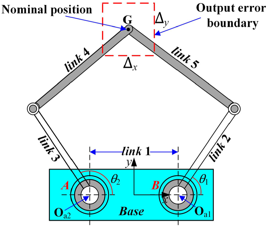
The planar five-bar mechanism.

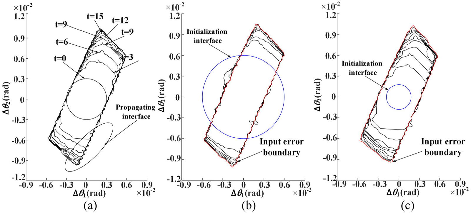
Here, the initial input error interface is set to be a small circle (radius: 0.003 rad), as presented in Figure 7(a). According to the “Searching the input error boundary” section, the input error interface will be propagated with the normal speed field defined by equation (13). Note that the adjustment coefficient $λ_{adjust}$ is set to 35 via plenty of numerical experiments. Figure 7(a) demonstrates the evolution of the input error propagating front at t = 0, 3, 6, 9, 12, and 15, respectively. Obviously, the exact boundary is obtained at t = 15.

Figure 7.

Propagation of the two-dimensional input error interface with different initial interfaces: cases (a), (b), and (c).

There might be some confusion about whether the initial interface affects the final result. To prove that it has no influence on the exact boundary, two different initial interfaces (see Figure 7(a) and (b)) are set to search the boundary again. It can be observed that the same boundary is obtained with different initial interfaces although the propagation times are different.

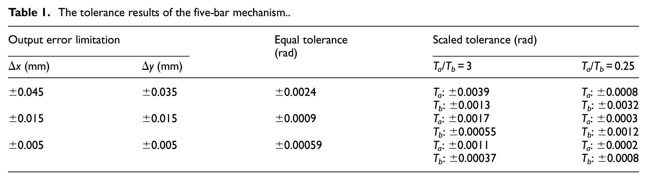
Now, the tolerance width of each input can be evaluated based on this boundary. For the equal principle, the tolerance bands of inputs A and B are both ±0.0024 rad (Figure 8(a)). For the scaled principle, two proportionality factors are assigned: if T_a/T_b = 3, the tolerance bands of A and B are ±0.0039 and ±0.0013 rad, respectively (see Figure 8(b)); if T_a/T_b = 0.25, that of A and B are ±0.0008 and ±0.0032 rad, respectively (see Figure 8(c)). Besides, another two numerical simulations are proceeded under different output error boundary. The whole results are listed in Table 1.

Figure 8.

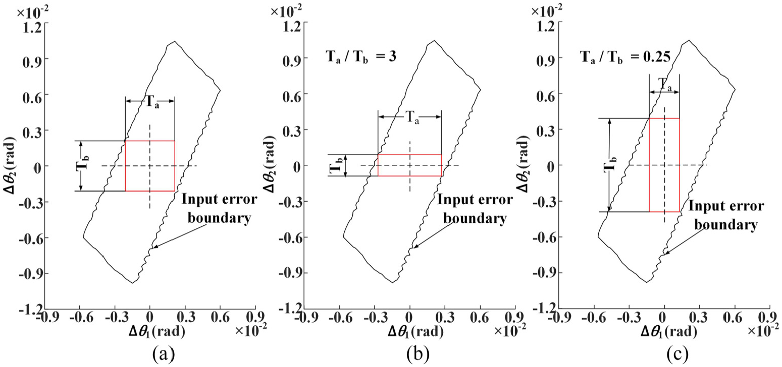
Input tolerance design for the 2-DOF five-bar parallel mechanism according to (a) the equal principle, and scaled principle with different proportionality factors of (b) T_a/T_b = 3 and (c) T_a/T_b = 0.25.

Table 1.

The tolerance results of the five-bar mechanism.

Output error limitation		Equal tolerance (rad)	Scaled tolerance (rad)
Δx (mm)	Δy (mm)	Equal tolerance (rad)	T_a/T_b = 3	T_a/T_b = 0.25
±0.045	±0.035	±0.0024	T_a: ±0.0039T_b: ±0.0013	T_a: ±0.0008T_b: ±0.0032
±0.015	±0.015	±0.0009	T_a: ±0.0017T_b: ±0.00055	T_a: ±0.0003T_b: ±0.0012
±0.005	±0.005	±0.00059	T_a: ±0.0011T_b: ±0.00037	T_a: ±0.0002T_b: ±0.0008

3-RPR parallel robot

Figure 9 gives the scheme of a 3-RPR planar parallel robot. This robot is designed as follows:³³

The translational actuators are mounted on the middle prismatic pairs;

Triangles P₀₁P₀₂P₀₃ and P₁P₂P₃ are equilateral;

OP_0i = 0.35 m and OP_i = 0.1 m (i = 1, 2, 3);

The origin of the local frame mounted on the mobile platform P₁P₂P₃ is located at the midpoint of P₁P₃ and the corresponding x-axis is alongside P₁P₃;

The origin of the global frame situates at point P₀₁, with x_g-axis pointing from P₀₁ to P₀₃.

The pose error of the mobile platform contains a rotational imperfection and two translational deviations along x_g and y_g directions, respectively. Therefore, the output error boundary is actually a 3D box (see Figure 9). When searching the input error boundary, the initial propagation interface at t = 0 is set to be a sphere (see Figure 10). The exact input error boundary is derived after 12 iterations.

Figure 9.

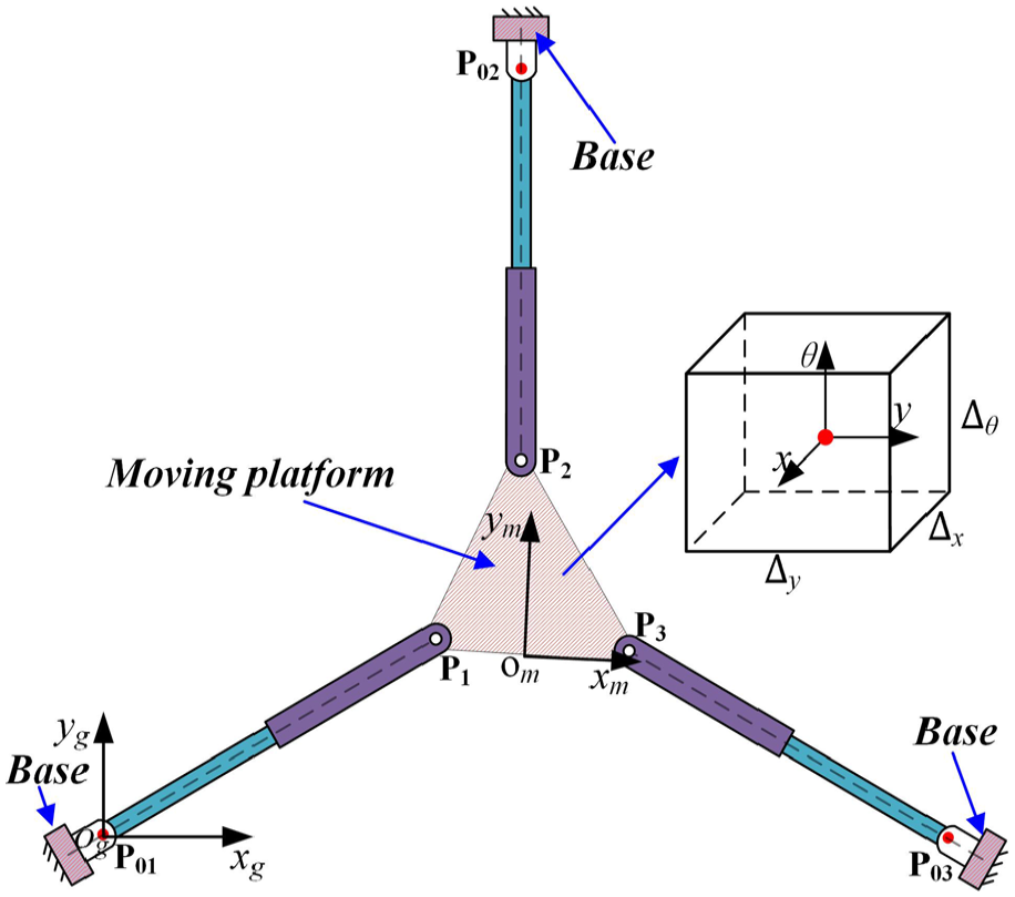
Diagram of the 3-RPR parallel mechanism.

Figure 10.

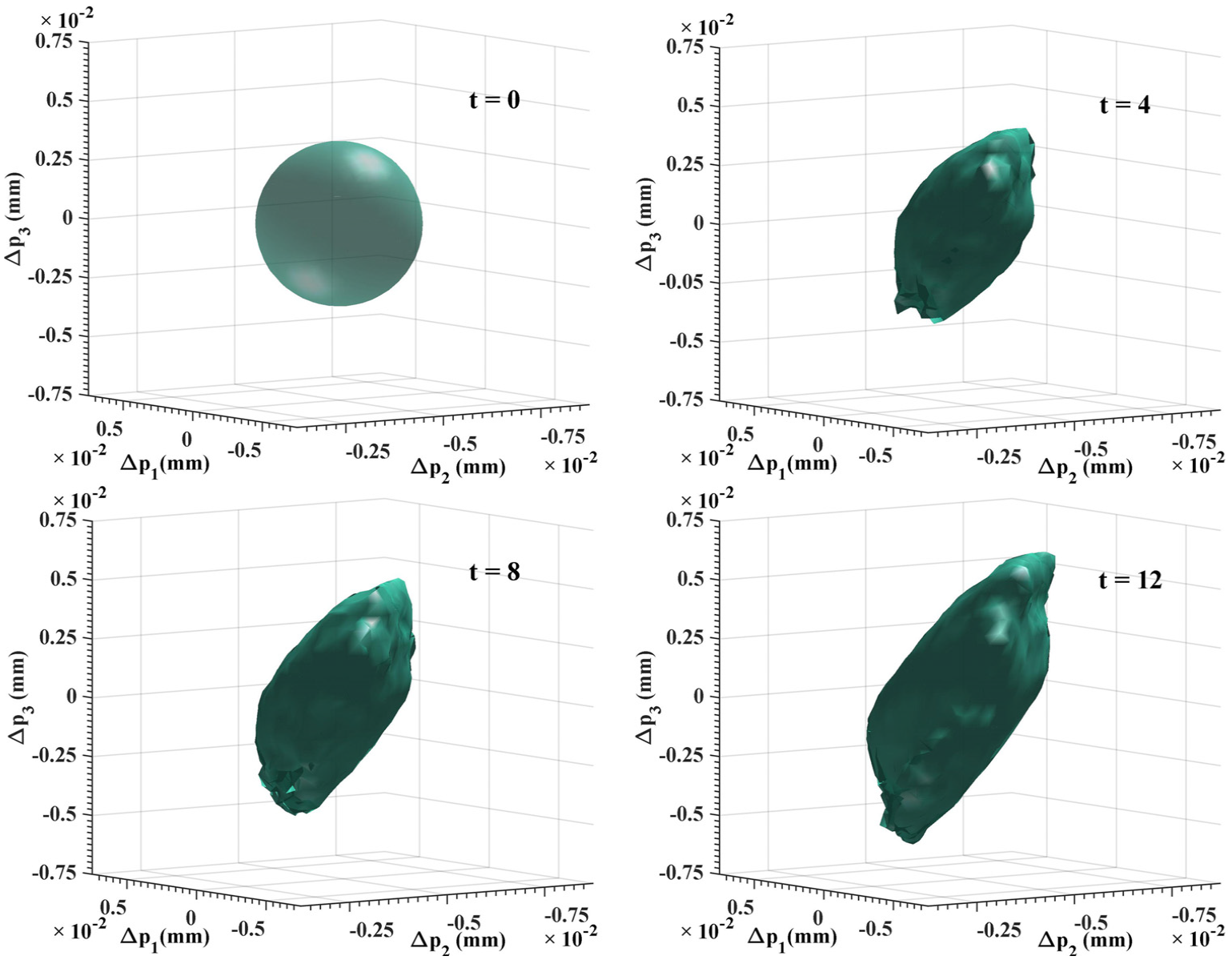
Evolution of the 3D input error interface.

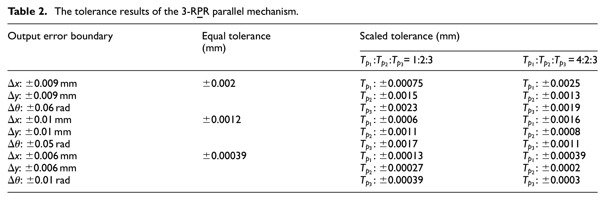
For the equal principle, the maximum cube (Figure 11(a)) should be looked for, whereas for the scaled principle, the maximum cuboid (Figure 11(b)) whose side ratio satisfies the design requirement should be sought. The tolerance results obtained in Figure 11 are constrained by the output error boundary as follows: |Δx| ≤ 0.009 mm, |Δy| ≤ 0.009 mm, and |Δθ| ≤ 0.009 rad. Likewise, another numerical simulations with different output error limitations are performed. The whole results are listed in Table 2.

Table 2.

The tolerance results of the 3-RPR parallel mechanism.

Output error boundary	Equal tolerance (mm)	Scaled tolerance (mm)
Output error boundary	Equal tolerance (mm)	$T_{p_{1}}$ : $T_{p_{2}}$ : $T_{p_{3}}$ = 1:2:3	$T_{p_{1}}$ : $T_{p_{2}}$ : $T_{p_{3}}$ = 4:2:3
Δx: ±0.009 mmΔy: ±0.009 mmΔθ: ±0.06 rad	±0.002	$T_{p_{1}}$ : ±0.00075 $T_{p_{2}}$ : ±0.0015 $T_{p_{3}}$ : ±0.0023	$T_{p_{1}}$ : ±0.0025 $T_{p_{2}}$ : ±0.0013 $T_{p_{3}}$ : ±0.0019
Δx: ±0.01 mmΔy: ±0.01 mmΔθ: ±0.05 rad	±0.0012	$T_{p_{1}}$ : ±0.0006 $T_{p_{2}}$ : ±0.0011 $T_{p_{3}}$ : ±0.0017	$T_{p_{1}}$ : ±0.0016 $T_{p_{2}}$ : ±0.0008 $T_{p_{3}}$ : ±0.0011
Δx: ±0.006 mmΔy: ±0.006 mmΔθ: ±0.01 rad	±0.00039	$T_{p_{1}}$ : ±0.00013 $T_{p_{2}}$ : ±0.00027 $T_{p_{3}}$ : ±0.00039	$T_{p_{1}}$ : ±0.00039 $T_{p_{2}}$ : ±0.0002 $T_{p_{3}}$ : ±0.0003

Figure 11.

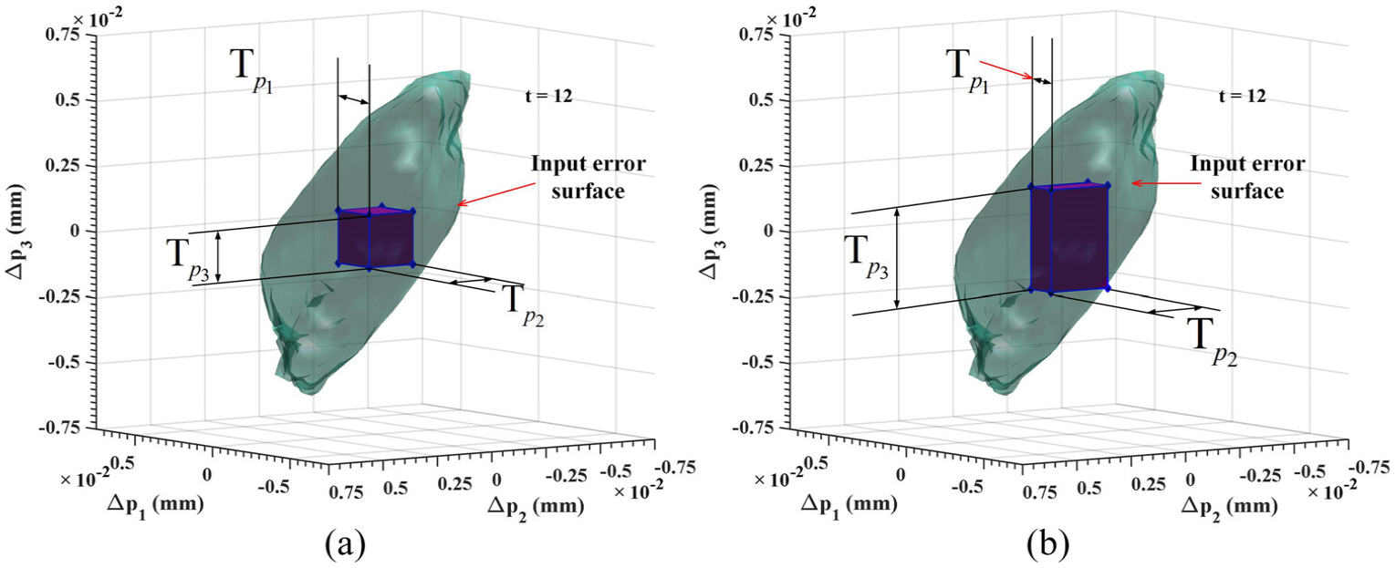
Input tolerance design within closed input error boundary for the 3-RPR parallel mechanism. (a) equal principle; (b) scaled principle.

Discussion

As mentioned above, the initial input error interface does not affect the final exact input error boundary, but it inevitably has influence on the convergence rate. According to Figure 7, it is evident that the larger initial input error interface needs a shorter time to achieve the exact boundary. In fact, the most appropriate initial input error curve can be chosen by several numerical experiments for the propagation. And also, it can be easily seen that as the output accuracy requirement becomes strict, namely, a tighter output error space, the input tolerance band will come about an obvious shrink, which is in accordance with the practical experience. In addition, for the 3-RPR parallel robot, there is an interesting point that the boundary of the angular error of the end-effector plays a more important role in the magnitude of the input tolerance than that of the positional ones (see Table 2). As a consequence, if there is a task imposing a high standard on the rotational accuracy of the end-effector, the actuator with a narrower backlash should be opted undoubtedly. More importantly, an imperceptible but apparent merit of the proposed method is that it is capable of presenting the tolerance results with a visualized geometry (see Figures 8 and 11), which is prohibitively intuitive and also provides a physical interpretation for the designer. Clearly, the previous optimization or stochastic methodologies cannot reach to this point. But, it should also be pointed out that compared to the planar case, the application of this method to the spatial parallel mechanism needs more intensive computation in that the dimension enlargement perplexes the judgment of the closeness between the practical and designed output error spaces. At the same time, since the mapping from the input error interface to the output counterpart is based on the forward kinematics, the proposed method will fail to be effective for the parallel mechanism suffering a forward singularity.

Conclusion

This study proposes a novel approach based on the level set method to implement the input tolerance design for parallel mechanisms. First, the input error boundary is obtained by means of the level set method, which inserts an initial error interface into a defined higher dimension level set function—distance function—and propagates it to evolve with a newly defined normal speed. Then, the evaluation of the tolerance width for each driving joint, according to different principles, is carried out in a geometric manner. Compared with the previous works that mostly regard tolerance design as a purely optimization problem, the contribution of this work, conversely, is transforming the evaluation of the input tolerance into a geometric issue, which is more straightforward and pellucid. Considering the level set method is available for evolving any dimensional hypersurface theoretically, this approach is generalized so that it can be applied to the spatial parallel mechanism except these situating at a forward singularity.

Footnotes

Appendix 1 Declaration of conflicting interests

The author(s) declared no potential conflicts of interest with respect to the research, authorship, and/or publication of this article.

Funding

The author(s) disclosed receipt of the following financial support for the research, authorship, and/or publication of this article: The authors are so grateful to the National Natural Science Foundation of China (Grant Nos 51635010 and 51805419) and the China Postdoctoral Science Foundation funded project (Grant No. 2018M631147) for the financial support of the work in this paper.

ORCID iD

Junkang Guo

References

Merlet

. Computing the worst case accuracy of a PKM over a workspace or a trajectory. In: Proceedings of the 5th Chemnitz parallel kinematics seminar, Chemnitz, 2006, pp.83–96, https://www.researchgate.net/publication/258844681_Computing_the_worst_case_accuracy_of_a_PKM_over_a_workspace_or_a_trajectory

Chebbi

Affi

Romdhane

LJM

, et al. Prediction of the pose errors produced by joints clearance for a 3-UPU parallel robot. Mech Mach Theory 2009; 44: 1768–1783.

Wang

Chen

Zhao

, et al. Output error bound prediction of parallel manipulators based on the level set method. Mech Mach Theory 2010; 45: 1153–1170.

Liu

Jin

Liu

, et al. Analytical method for optimal component tolerances based on manufacturing cost and quality loss. Proc IMechE, Part B: J Engineering Manufacture 2013; 227: 1484–1491.

Cheng

Tsai

JC.

Optimal statistical tolerance allocation for reciprocal exponential cost–tolerance function. Proc IMechE, Part B: J Engineering Manufacture 2013; 227: 650–656.

Chase

Greenwood

WH.

Design issues in mechanical tolerance analysis. Manuf Rev 1988; 1: 50–59.

Dong

Xue

New production cost-tolerance models for tolerance synthesis. J Eng Ind 1994; 116: 199–206.

Govindarajalu

Karuppan

Manoharan

Tolerance design of mechanical assembly using NSGA II and finite element analysis. J Mech Sci Technol 2012; 26: 3261–3268.

Vignesh Kumar

Ravindran

Lenin

, et al. Tolerance allocation of complex assembly with nominal dimension selection using Artificial Bee Colony algorithm. Proc IMechE, Part C: J Mechanical Engineering Science 2019; 233: 18–38.

10.

Muthu

Dhanalakshmi

Sankaranarayanasamy

Optimal tolerance design of assembly for minimum quality loss and manufacturing cost using metaheuristic algorithms. Int J Adv Manuf Technol 2009; 44: 1154–1164.

11.

Krishna

Rao

KM.

Simultaneous optimal selection of design and manufacturing tolerances with different stack-up conditions using scatter search. Int J Adv Manuf Technol 2006; 30: 328–333.

12.

Jawahar

Sivasankaran

Ramesh

Optimal Pareto front for manufacturing tolerance allocation model. Proc IMechE, Part B: J Engineering Manufacture 2017; 231: 1190–1203.

13.

Shao

Zhang

, et al. Error modeling and tolerance design of a parallel manipulator with full-circle rotation. Adv Mech Eng 2016; 8: 1687814016649300.

14.

Lin

Chan

Lee

JJ.

Kinematic error analysis and tolerance allocation of cycloidal gear reducers. Mech Mach Theory 2018; 124: 73–91.

15.

Polini

Geometric tolerance analysis. In: Colosimo

Senin

(eds) Geometric tolerances: impact on product design, quality inspection and statistical process monitoring. London: Springer, 2011, pp.39–68.

16.

Desrochers

Clément

A dimensioning and tolerancing assistance model for CAD/CAM systems. Int J Adv Manuf Technol 1994; 9: 352–361.

17.

Gao

Chase

Magleby

SP.

Generalized 3-D tolerance analysis of mechanical assemblies with small kinematic adjustments. IIE Trans 1998; 30: 367–377.

18.

Giordano

Samper

Petit

. Tolerance analysis and synthesis by means of deviation domains, axi-symmetric cases. In: Davidson

(ed.) Models for computer aided tolerancing in design and manufacturing. Dordrecht: Springer, 2007, pp.85–94.

19.

Bourdet

Mathieu

Lartigue

, et al. The concept of the small displacement torsor in metrology. Adv Math Tool Metrol 1996; 40: 110–122.

20.

Mahshid

Mansourvar

Hansen

HN.

Tolerance analysis in manufacturing using process capability ratio with measurement uncertainty. Precis Eng 2018; 52: 201–210.

21.

Jiang

Davidson

Liu

, et al. Using tolerance maps to validate machining tolerances for transfer of cylindrical datum in manufacturing process. Int J Adv Manuf Technol 2014; 73: 465–478.

22.

Kumaraswamy

Shunmugam

Sujatha

A unified framework for tolerance analysis of planar and spatial mechanisms using screw theory. Mech Mach Theory 2013; 69: 168–184.

23.

Goldsztejn

Caro

Chabert

A three-step methodology for dimensional tolerance synthesis of parallel manipulators. Mech Mach Theory 2016; 105: 213–234.

24.

Zhang

Liu

Ding

, et al. Tolerance analysis of annular surfaces considering form errors and local surface deformations. Proced CIRP 2018; 75: 291–296.

25.

Homri

Goka

Levasseur

, et al. Tolerance analysis—form defects modeling and simulation by modal decomposition and optimization. Comput Aid Des 2017; 91: 46–59.

26.

Armillotta

Force analysis as a support to computer-aided tolerancing of planar linkages. Mech Mach Theory 2015; 93: 11–25.

27.

Mazur

Leary

Subic

Application of polynomial chaos expansion to tolerance analysis and synthesis in compliant assemblies subject to loading. J Mech Design 2015; 137: 031701.

28.

Corrado

Polini

Assembly design in aeronautic field: from assembly jigs to tolerance analysis. Proc IMechE, Part B: J Engineering Manufacture 2017; 231: 2652–2663.

29.

Cao

Liu

Yang

, et al. A novel tolerance analysis method for three-dimensional assembly. Proc IMechE, Part B: J Engineering Manufacture 2018; 233: 1818–1827.

30.

Singh

Jain

Important issues in tolerance design of mechanical assemblies. Part 1: tolerance analysis. Proc IMechE, Part B: J Engineering Manufacture 2009; 223: 1225–1247.

31.

Singh

Jain

SC.

Important issues in tolerance design of mechanical assemblies. Part 2: tolerance synthesis. Proc IMechE, Part B: J Engineering Manufacture 2009; 223: 1249–1287.

32.

Kim

Choi

YJ.

The kinematic error bound analysis of the Stewart platform. J Field Robot 2015; 17: 63–73.

33.

Kroger

Binder

Accuracy analysis of 3-DOF planar parallel robots. Mech Mach Theory 2008; 43: 445–458.

34.

Osher

Sethian

JA.

Fronts propagating with curvature-dependent speed: algorithms based on Hamilton-Jacobi formulations. J Comput Phys 1988; 79: 12–49.

35.

Sethian

Smereka

Level set methods for fluid interfaces. Annu Rev Fluid Mech 2003; 35: 341–372.

36.

Allaire

Jouve

Toader

AM.

Structural optimization using sensitivity analysis and a level-set method. J Comput Phys 2004; 194: 363–393.

37.

Chan

Vese

LA.

Active contours without edges. IEEE Trans Image Process 2001; 10: 266–277.

38.

Peng

Merriman

Osher

, et al. A PDE-based fast local level set method. J Comput Phys 1999; 155: 410–438.

39.

Andrew

AM.

Level set methods and fast marching methods: evolving interfaces in computational geometry, fluid mechanics, computer vision, and materials science (2nd edition). Kybernetes 2000; 29: 239–248.

40.

Geetha