
Abstract
Synergistic improvement on low carbon manufacturing is not taken full consideration in flow shop scheduling in literatures. To fill the gap, this article extends a flow shop scheduling problem by considering low carbon emission and variable machining parameters. The difference between the extended scheduling problem and the traditional one is that the former investigates the comprehensive effects of machine and scheduling levels on production throughput and environmental impact. A mathematical model of the extended problem is formulated to find the Pareto frontier, which is the set of scheduling solutions that are all Pareto efficient. Moreover, two problem-specific scheduling methods are presented and their effects on the considered problem are proved. A novel multi-objective heuristic is developed to deal with the extended problem because it is a non-deterministic polynomial acceptable problem. An actual case is studied to demonstrate the feasibility and applicability of the proposed extended problem and two scheduling methods. These finds can be employed in manufacturing execution systems and do not require additional cost.
Keywords
Introduction
It is well known that global warming stems from the increasing amount of greenhouse gas due to the soaring energy consumption. In China, a National Climate Change Plan was proposed with a goal to reduce the carbon emission intensity by 40%–45% by 2020 from the 2005 level. Similar regulations were laid down in other countries and regions, including the United States, European Union, Japan, and so on.
There are two practical approaches for reducing carbon emission in manufacturing: one is to use energy-saving equipment and embodied energy framework, 1 and the other is to employ low carbon operational strategies and optimization methods. 2 The former needs a large capital investment to develop new technologies and replace old equipment, while the latter requires less cost and is more preferred by manufacturers.
Recently, extensive studies on energy saving or low carbon in manufacturing scheduling systems are found. Mouzon et al. 3 observed a fact that there were a large amount of energy savings when idle machines were turned off. In their follow-up work, a single machine scheduling model with the objectives of minimizing energy consumption and tardiness was reported. 4 Their model adopted an “ON–OFF” method, which switches machines off when they are idle and switches them on before new workpieces come. Fang et al. 5 used a speed scaling method in a flow shop scheduling problem with a peak power constraint. It is assumed that machines can run at varying speed levels and more energy is consumed if a machine works at a higher speed. Thus, it is possible to reduce energy consumption by slowing down some operations.
According to the studies,6,7 carbon emission of any machining operation is concerned with energy consumption, resource utilization, and waste disposal. Carbon emission is a more overall criterion to indicate the environmental burden of manufacturing activities when compared with energy consumption. In the carbon efficient scheduling model proposed by Ding et al., 8 carbon emission was only tied to energy consumption. However, they neglected the carbon emission caused during the preparation time and tool motion time of operations. A special blocking flow shop scheduling case in turning processes for high efficiency and low carbon was investigated in Lin et al.’s 9 work.
Synergistic improvement can be achieved by considering the integrated optimization of multiple perspectives.10,11 However, no much work was reported to investigate the integrated optimization. In the speed scaling method, machines only run at several prespecified levels.5,8,12 It may not be practical in some manufacturing systems, as machine tools can run at any speed in a range. Besides, as other machining parameters (i.e. feed rate and depth of cut) also have impacts on carbon emission, 13 they should be considered in the integrated optimization. To fill the gap, this article addressed a flow shop scheduling problem with variable machining parameters. The contribution of this work can be summarized as follows: (1) development of a novel multi-objective mathematical model, taking into account the machining parameters and the scheduling sequence as decision variables; (2) presentation of two problem-specific scheduling methods that aim to cut down carbon emission in scheduling; and (3) demonstration of the effects of the synergistic use of methods on Pareto frontier and the importance of the order of using them in optimization procedures.
The remainder of this article is organized as follows. A carbon emission calculation method for machining operations is introduced in section “Carbon emission calculating method,” while the mathematical model of a flow shop scheduling problem with variable machining parameters is briefly described in section “Flow shop scheduling problem with variable machining parameters.” Section “Problem-specific scheduling methods” gives two scheduling methods and section “Modified multi-objective GWO” presents a modified multi-objective grey wolf optimizer (GWO). Finally, sections “Case study” and “Conclusion” present the analysis of a case study and the conclusion, respectively.
Carbon emission calculating method
As the carbon emission due to workpiece (chips) is determined at the stage of production design or process design, they are not considered during machining parameter optimization (MPO) and scheduling. Carbon emission in a machining operation, denoted by Cms (g), is mainly caused by electricity consumption, cutting tools, and cutting fluid. 14 It can be calculated as follows

where Celec (g), Ctool (g), and Cfluid (g) are carbon emission due to electricity consumption, cutting tools, and cutting fluid in a machining operation, respectively.
Celec
Celec has a linear relationship with energy consumption, denoted by Eelec (kJ), in a machining operation, and can be determined as follows

where Felec is the electricity carbon emission factor. Felec is obtained from the study conducted by Department of National Development and Reform Commission in China in 2011. The average value of six grids in China is 0.1524 g CO2/kJ. 15
Three states are observed in a machining operation: “basic state,”“ready state,” and “cutting state.” 16 Given a machining operation with Nstep passes, Eelec can be represented as follows
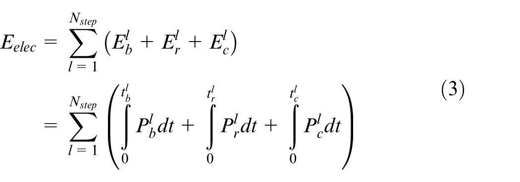
where
In the basic state, a constant value of power is consumed.

where Pb is the power consumption (kW) in the basic state.
In the ready state, the power consumption, denoted by Pp (kW), consists of two parts: Pb and the operational power Pop. 16 The latter has a linear relationship with the spindle speed, denoted by n (r/min)

where k1 and k2 are the regression coefficients.
Then,

Li and Kara
17
reported a specific energy consumption model to estimate

where
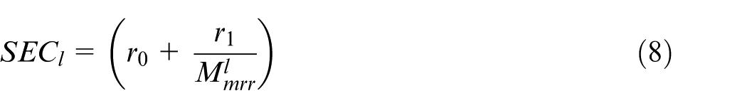
where
The formulae of
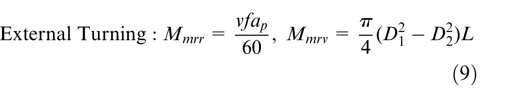
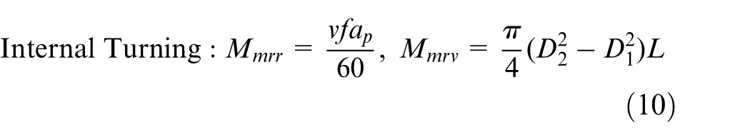
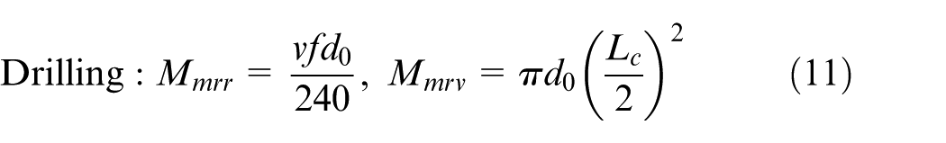
where v, f, ap are the cutting velocity (m/min), feed rate (mm/r), and depth of cut (mm), respectively. D1 and D2 are the workpiece diameters before and after machining, respectively. L is the cutting length. d0 is the tool diameter, and Lc is the depth of drilling.
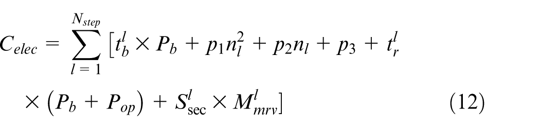
Substituting Celec in equations (3)–(7), Celec can be re-expressed as follows
Ctool and Cfluid
Carbon emission caused by cutting tools, denoted by Ctool (g), can be calculated as follows 13
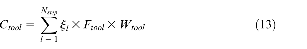
where ξl is the used tool life in the lth pass, Ftool (g CO2/g) is the tool carbon emission factor, and Wtool (g) is the tool mass. ξl is given as follows
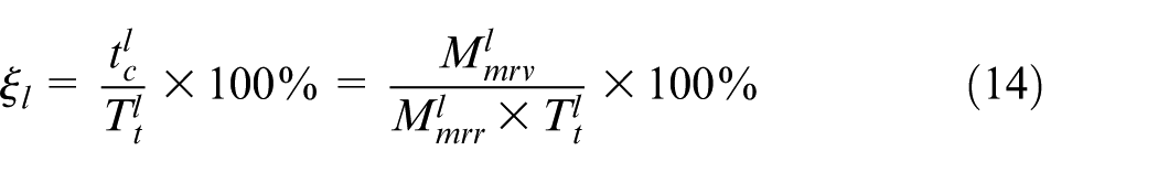
where

where N is the times of re-sharpening and
Carbon emission caused by cutting fluid, denoted by Cfluid (g), can be calculated as follows 6
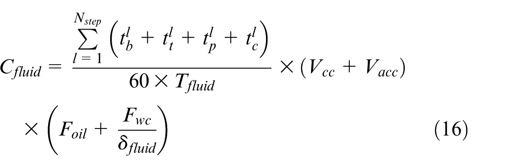
where Foil (g CO2/L) is the cutting fluid carbon emission factor, Fwc (g CO2/L) is the carbon emission factor of cutting fluid disposal. Vcc (L) and Vacc (L) are the initial volume and additional volume of cutting fluid, respectively. δfluid and Tfluid (min) are the concentration and replace cycle of cutting fluid, respectively.
Flow shop scheduling problem with variable machining parameters
The flow shop scheduling problem with variable machining parameters (FVP) is an extended version of a flow shop scheduling problem (FSP). An FVP model owns a two-level structure, that is, the lower level is a MPO sub-model and the upper level is an FSP sub-model.
MPO sub-model
The optimization objectives of the MPO sub-model are machining time tms and carbon emission Cms. Generally, a specific value of the depth of cut is determined by the workpiece’s process and the machining allowance, and that of the width of cut is determined by the rigidity of tools, machines, and workpieces. Therefore, the cutting velocity and feed rate are considered as decision variables in the sub-model.
Assume that operation Oij has
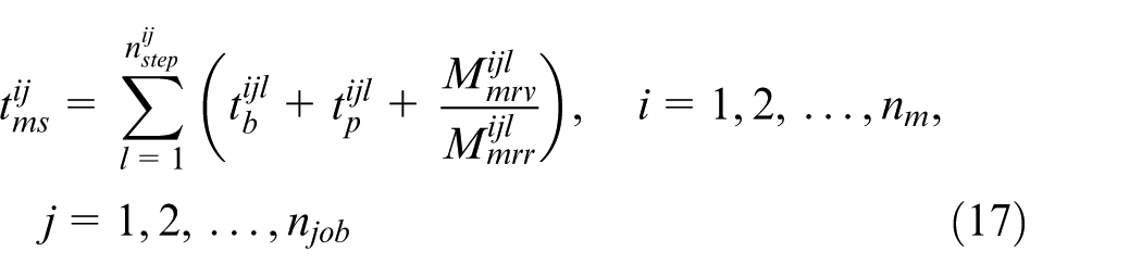
where
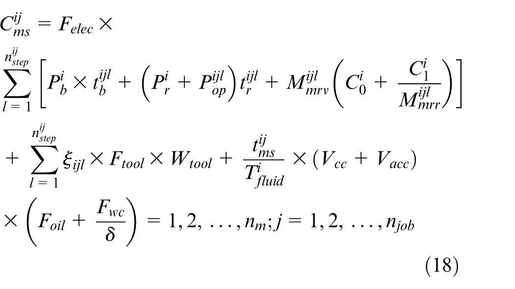
According to equations (12), (13), and (16), carbon emission of Oij can be calculated as follows
It should be ensured that the machining parameters are in their upper and lower bounds, that is
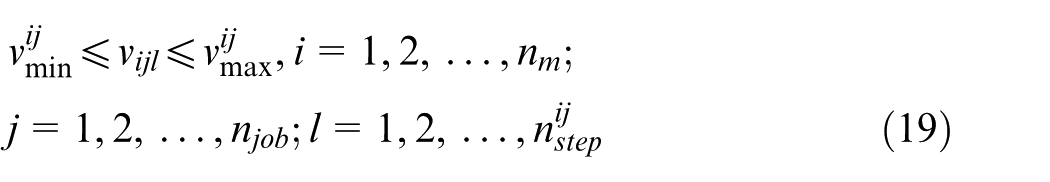
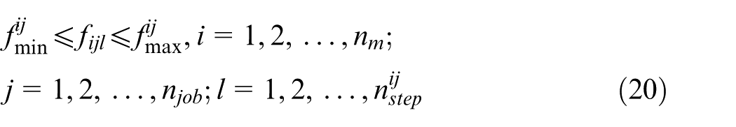
where
FSP sub-model
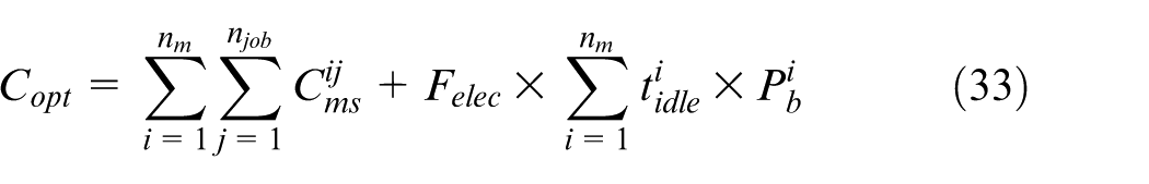
The optimization objectives of the FSP sub-model are makespan Tmax(π) and carbon emission Copt. The “ON–OFF” method switches machines on before their first operations and switches them off after their last operations.
Then, the details of the FSP sub-model are presented as follows:
Optimization objectives
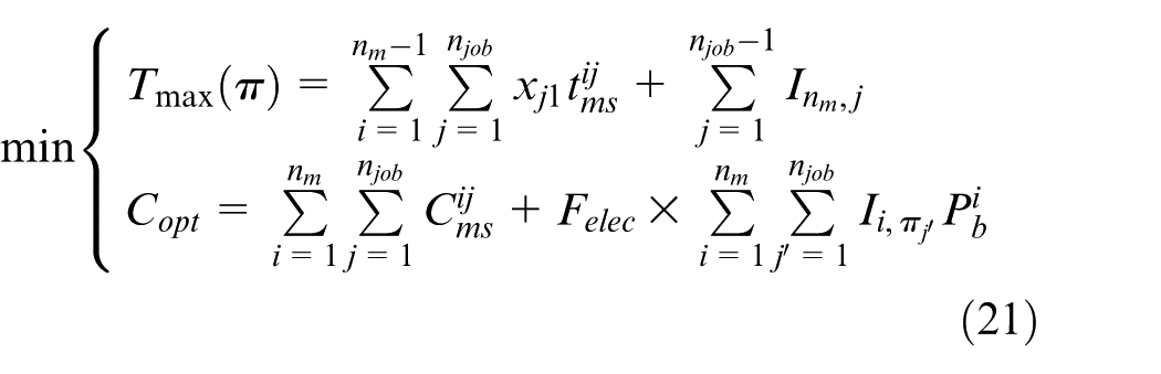
With constraints

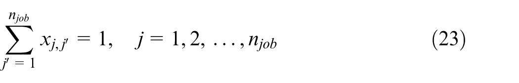
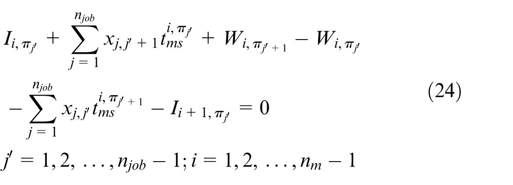


where πj′ is the j′th workpiece in π,
It is obvious that each position in the schedule should contain just one workpiece and each workpiece should be assigned to only one position, which is supported by constraints (22) and (23). Constraint (24) is incorporated into the model to calculate the idle times.
According to the two sub-models, a feasible solution can be expressed by a schedule π and a matrix of machine parameter combinations Mmpc as follows

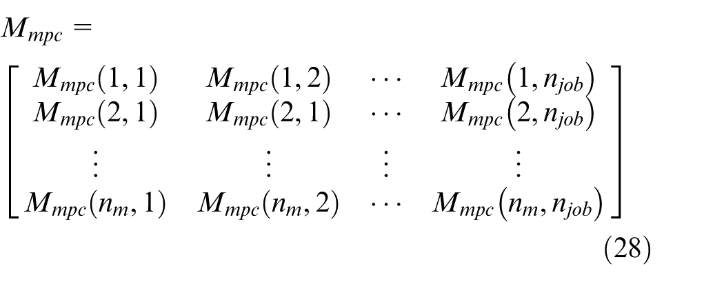
where the elements in π are the subscripts of workpieces, and Mmpc(i, j) is a combination of machining parameters for Oij.
Problem-specific scheduling methods
Two problem-specific scheduling methods are proposed in this article: postponing and improved two-stage optimization methods.
Postponing method
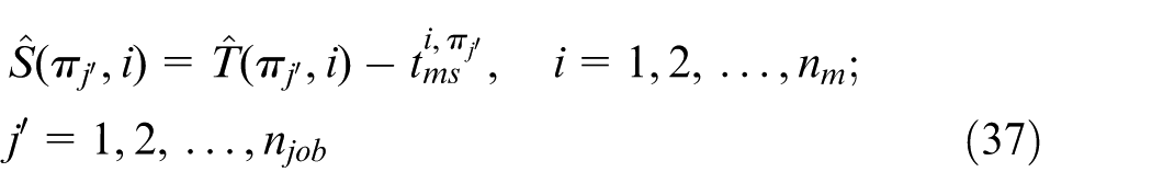
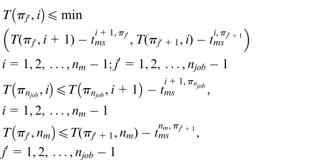
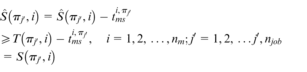
A postponing method is designed to postpone the processing of a workpiece as late as possible. Let T(πj′, i) and S(πj′, i) denote the completion time and start time of
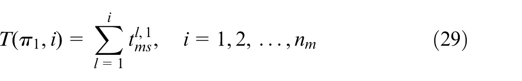
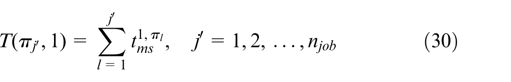
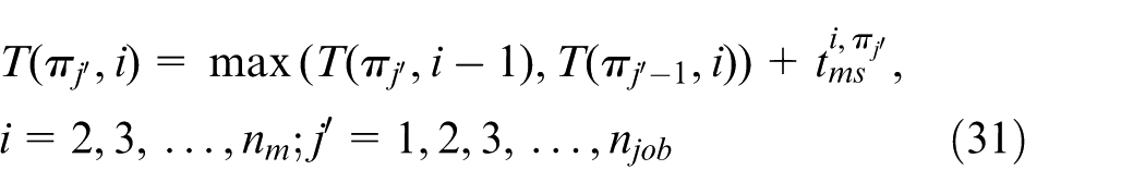
S(πj′, i) is equal to
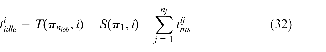
According to equation (32),
Let

Property 1
If the postponing method is employed on a solution, the original solution will be dominated by or equivalent to the improved solution.
Proof
The following equations are inferred from equations (29)–(31)
Thus
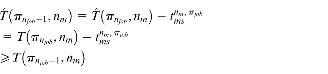
Then, it can be inferred that
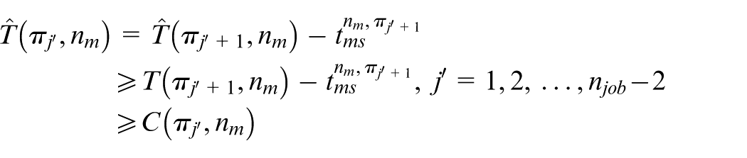
Similarly, it can be proved that
Therefore, the following equation can be inferred
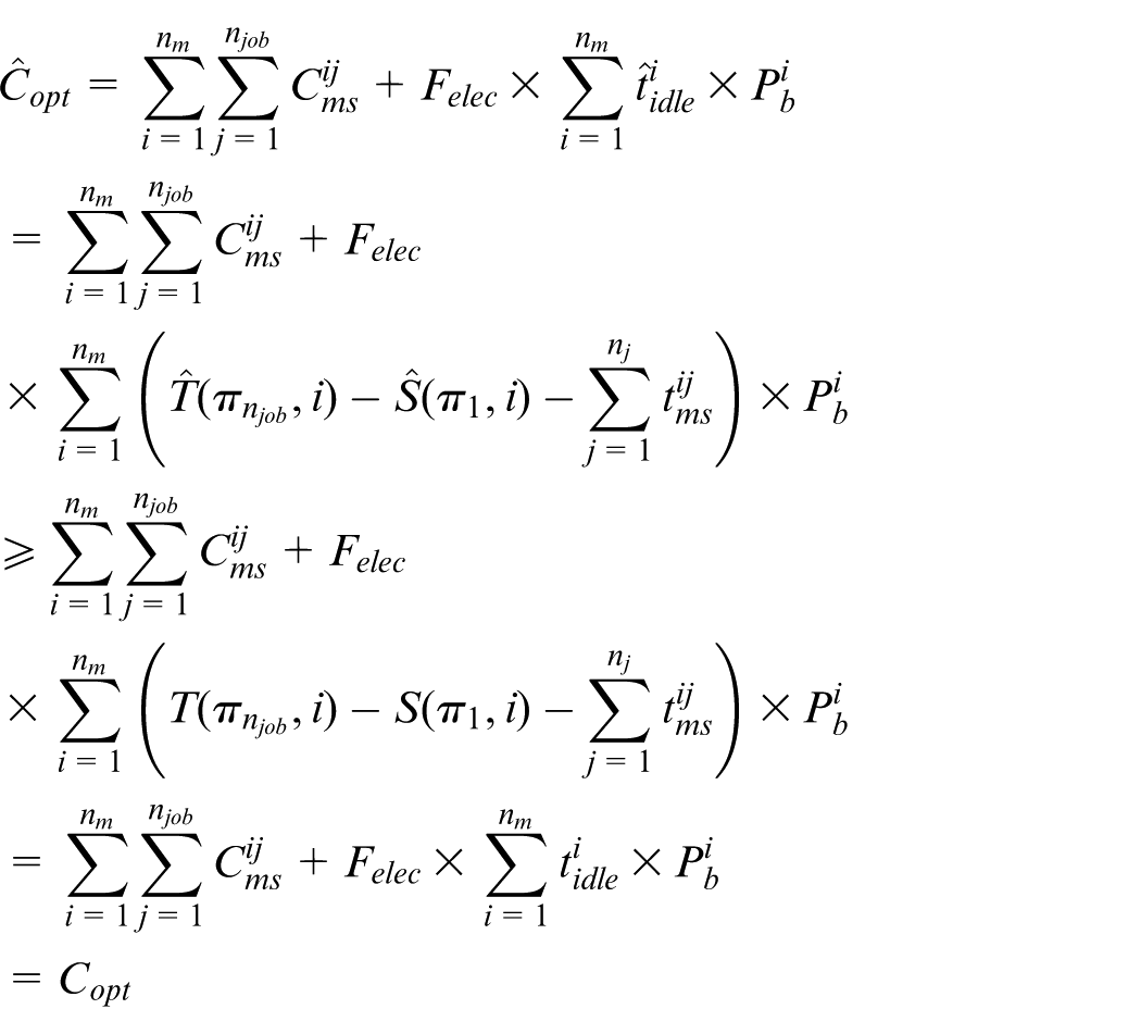
According to equation (34),
Improved two-stage optimization method
As machining parameters can be set to any values in their bounds, there exist a large amount of possible combinations of them. Fortunately, all combinations are dominated by the Pareto-optimal combinations in the Pareto frontier, denoted by Γ. Moreover, Γ can be easily obtained by optimizing the MPO sub-model. In Γ, the machining time of an operation decreases but the carbon emission increases, and vice versa. Based on the fact, the following property can be proved.
Property 2
Given a solution
Proof
Let

Therefore
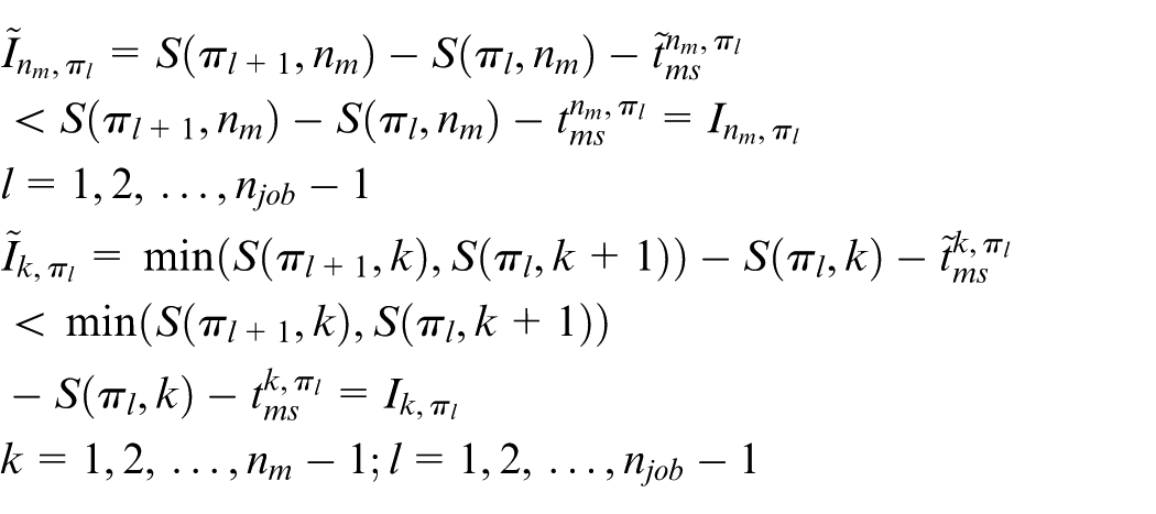
Thus,
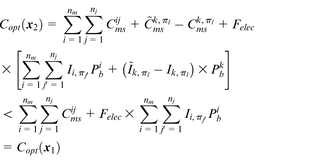
As the makespan is fixed, it can be concluded that
Based on Property 2, the steps of the improved two-stage optimization method are illustrated as follows:
Step 1. Get the Pareto frontier of each MPO sub-model and sort the Pareto-optimal combinations in an ascending order of their machining time.
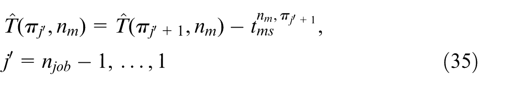
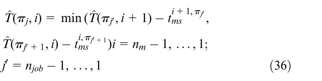
Step 2. Calculate the maximum machining time increment of each operation without affecting the makespan, denoted by Δ. The calculation formulae are
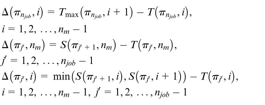
where
Step 3. Identify the Pareto-optimal combination in the Pareto frontier which owns the minimum carbon emission and satisfies the following equation for each operation
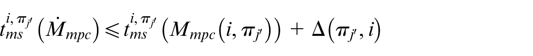
where
Step 4. The current combinations are replaced with the identified combinations, then the machining time and carbon emission are calculated for the new solution.
Modified multi-objective GWO
GWO is a novel nature-inspired population-based meta-heuristics, which is inspired by the hunting activities of grey wolves and has been proved to be of effectiveness and efficiency. 18 Furthermore, GWO is more self-adaptive, as no pre-determined parameters are required in it except the population size and maximum number of loops. A discrete multi-objective GWO (D-MOGWO) is described as follows.
Largest order-value-based encoding scheme
As π is a sequence of discrete values and Mmpc is a matrix of continuous values, a suitable mapping should be defined between π and a continuous-value sequence. Thus, a largest order-value rule 19 is proposed to fill the gap.
Non-dominated solution archive
The optimization goal of multi-objective problems is to find the entire Pareto-optimal set or its subset. In order to reach the goal, a non-dominated solution archive 20 is integrated in D-MOGWO. The archive is constructed at the beginning of each loop and involves two parts: the archive controller and adaptive grid procedure.
The archive controller is used to construct the archive. For each solution
The adaptive grid procedure is used to strengthen the diversity of the non-dominated solutions in the archive. The kernel idea is to divide the objective function grid of the non-dominated solutions into hyper-cubes. The procedure is re-performed when the new inserted solution lies outside the current grid. The crowding levels of hyper-cubes depend on the number of solutions in them. When the archive is full, a randomly selected solution in the most crowding hyper-cube is abandoned.
Roulette-wheel-based solution selection approach
In the basic GWO, the fittest solution in the current population is denoted by the alpha (α) wolf, and the second and third fittest solutions are denoted by the beta (β) and delta (δ) wolves, respectively. As no traditional fittest solution is available in a multi-objective optimization problem, a roulette-wheel-based solution selection approach is required in D-MOGWO. Each hyper-cube in the grid is assigned a selection probability pi as follows
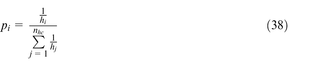
where hi is the number of solutions lie in the ith hyper-cubes and nhc is the number of hyper-cubes.
A roulette-wheel procedure is used to choose three hyper-cubes, and then a solution is randomly selected from each hyper-cube.
The rest in the population are conceived as omega (ω) wolves, and they follow the α, β, δ wolves in the hunting.
Main loop of D-MOGWO
Following equations are used to resemble the hunting activities 18


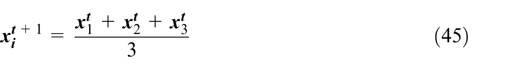
where


where the elements of
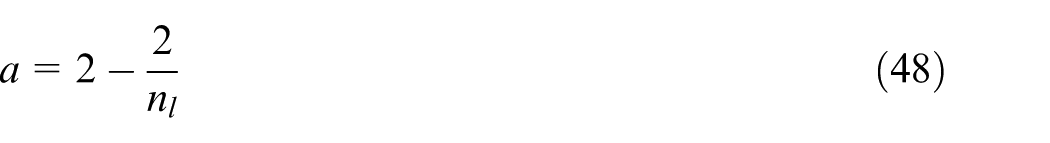
where nl is the maximum number of loops.
The flow chart of the D-MOGWO is shown in Figure 1.
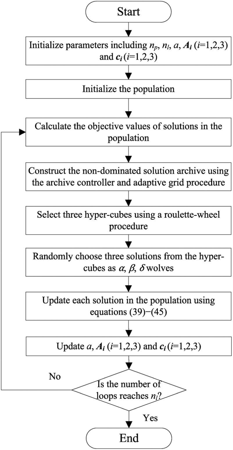
Flow chart of D-MOGWO.
Case study
Consider an eight-workpiece and three-machine FVP case. The diagram of the workpieces is shown in Figure 2. As shown in Table 1, eight different workpieces resulted from the combination of two different outer/inner diameters, two different lengths, and two different numbers of holes. Each workpiece requires three machining operations (i.e. external turning, internal turning, and drilling), and these operations are performed in a CNC lathe CK60 (M1), a CNC lathe CK0628 (M2), and a CNC drilling machine (M3) successively.
Dimensions of workpieces.
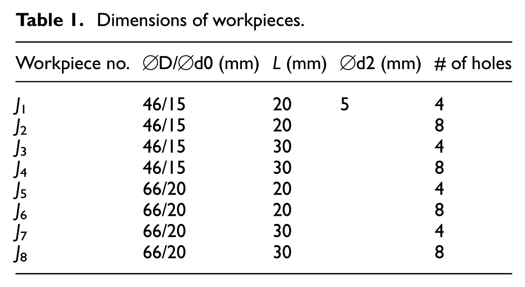
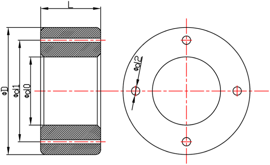
Diagram of workpieces.
The formulae of


where Cv, xv, yv, and m are the empirical coefficients related to the tool and workpiece materials.
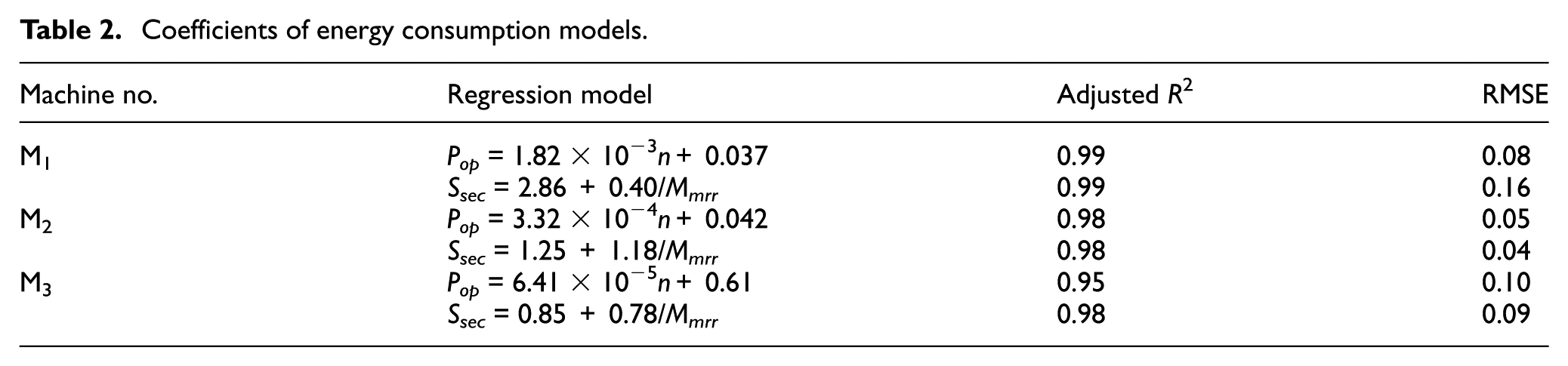
The energy consumption regression models of these machines were established based on experimental data. The three-level orthogonal array method was used, and nine tests were need for the experiment. Then, the energy consumption regression models were established using the multiple linear regression method and are depicted in Table 2. Figure 3 gives the regression result of the SEC model of M2. It shows that the empirical model was able to successfully predict the SEC. Pb was obtained using the sliding filter method and the values of Pb of these machines are 0.374, 0.418, and 0.473 kW, respectively. For details of the experiment, readers can refer to the authors’ previous works.14,21
Coefficients of energy consumption models.
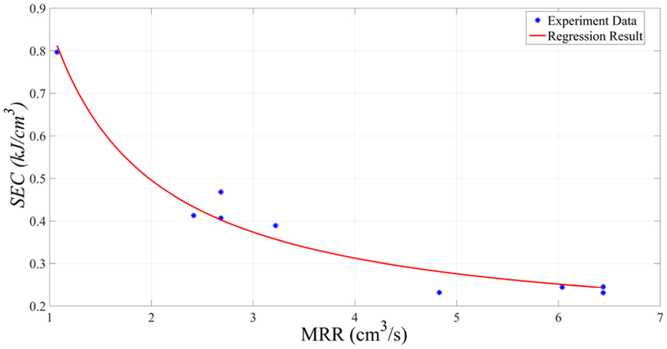
The SEC model of M2.
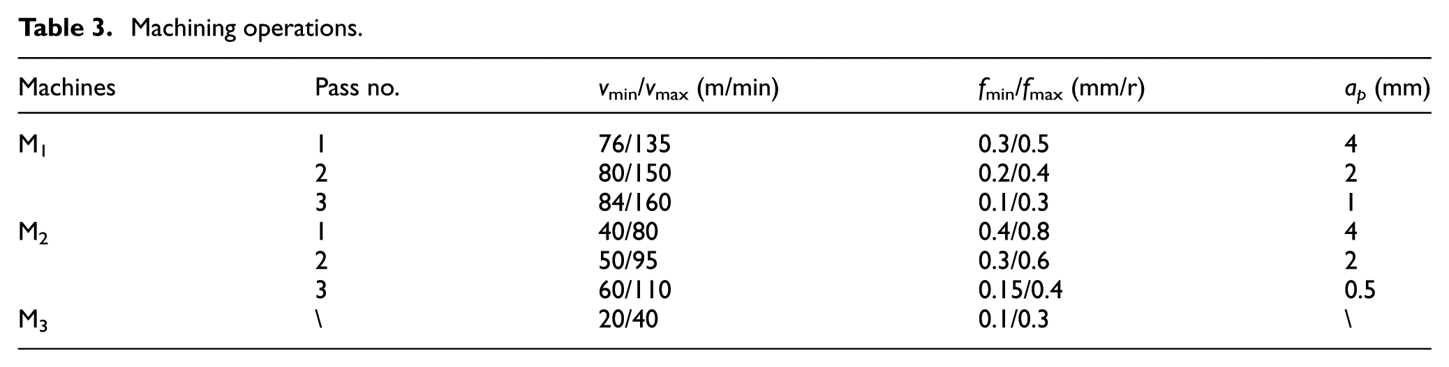
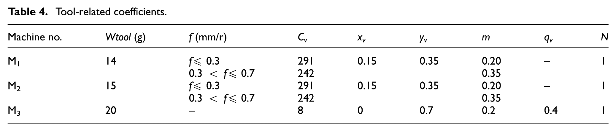
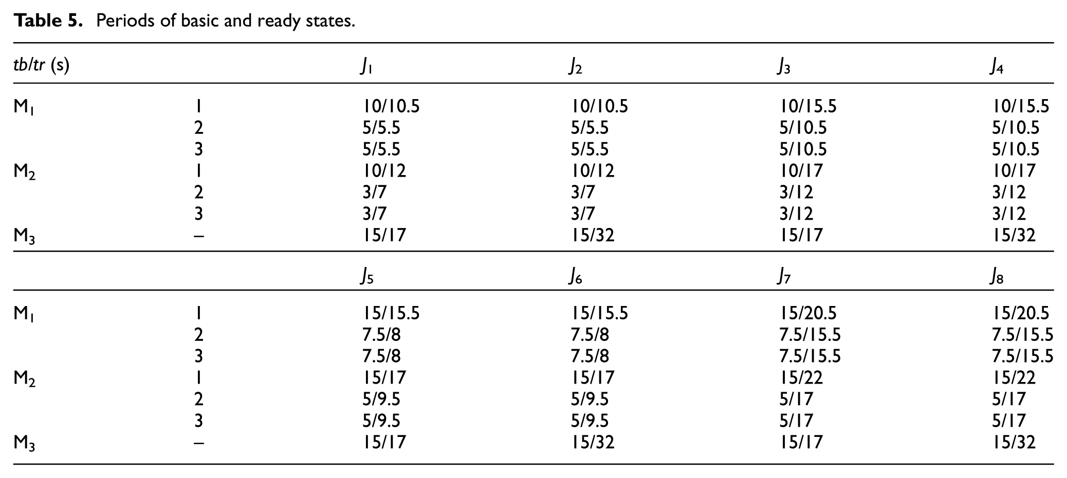
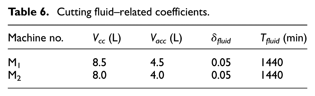
Details of the operations and machining parameters are given in Table 3.22,23 All of the machines are equipped with cemented carbide tools, the workpiece material is carbon steel, and the related constants and coefficients are listed in Table 4.22,23 The value of Ftool is 29.6 g CO2/g. 6 The period-related coefficients are given in Table 5. Both of the lathes use cutting fluid, and the drilling machine does not. The cutting fluid–related coefficients are listed in Table 6, and the values of Foil and Fwc are 2.85 and 0.2 g CO2/L, respectively.
Machining operations.
Tool-related coefficients.
Periods of basic and ready states.
Cutting fluid–related coefficients.
Algorithm setting and performance metrics
D-MOGWO was coded in MATLAB R2015b in a personal computer using a 64-bit Windows 7 operating system, a Pentium Dual-Core processor, and a 4-GB RAM. The population size and the maximum number of loops are set to 500 and 200, respectively.
In order to evaluate the effectiveness of the proposed methods, following performance metrics are considered:
Coverage metric: 24 this criterion provides a binary measure that determines which of two Pareto frontier Γ1 and Γ2 is better. It counts the percentage of solutions in Γ1 that are dominated by those in Γ2 and can be calculated as follows
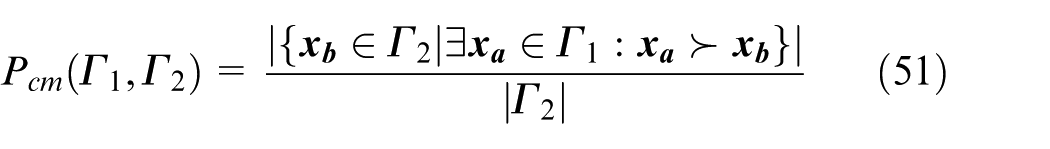
where
2. Spacing metric: 25 this criterion measures the extent of spread in the obtained Pareto frontier Γ. Let di denote Euclidean distance between solution i and its nearest solution. The spacing metric of Γ can be calculated as follows
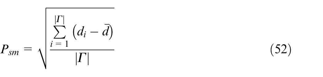
where Psm is the value of spacing metric, |Γ| is the number of solutions in Γ, and
D-MOGWO versus NSGA-II
To evaluate the effectiveness of the proposed heuristic, D-MOGWO is compared with NSGA-II, which is one of the most popular heuristic. The latter uses a non-dominated sorting and crowding distance and crowding distance calculating procedures. For NSGA-II, the population size is 500, the maximum number of loops is 200, the crossover rate is 0.9, and the mutation rate is 0.1. Each heuristic runs 30 times.
The performance metrics of the Pareto frontiers obtained by two heuristics are depicted in Figure 4. The part labels were described in sub-section “Algorithm settings and performance metrics”. For example, Pcm(NSGA-II, D-MOGWO) denotes the coverage metric of the Pareto frontier obtained by NSGA-II over that obtained by D-MOGWO. It is observed from the figure that the D-MOGWO outperforms NSGA-II for both performance metrics. The average of Pcm(D-MOGWO, NSGA-II) is 0.526, which means the majority of solutions in the Pareto frontier obtained by NSGA-II are dominated by D-MOGWO. The minimum, maximum, and average of Psm(D-MOGWO) are smaller than those of Psm(NSGA-II), respectively. The adoption of the roulette-wheel-based solution selection approach can improve the quality of population since the search process is guided by three randomly selected solutions. Therefore, it can be concluded that the D-MOGWO is effective in solving the proposed problem.
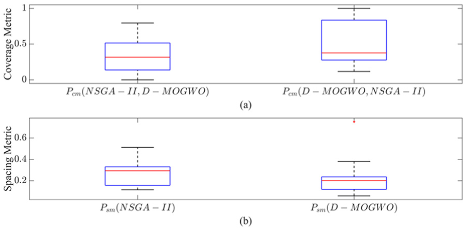
Performance metrics of the Pareto frontiers obtained by two heuristics.
Analysis of problem-specific scheduling methods
For the sake of simplicity, the postponing, two-stage optimization, 9 and improved two-stage optimization methods are denoted by A, B, and C, respectively. Several tests are generated due to using different methods in the considered case.
Effectiveness of methods
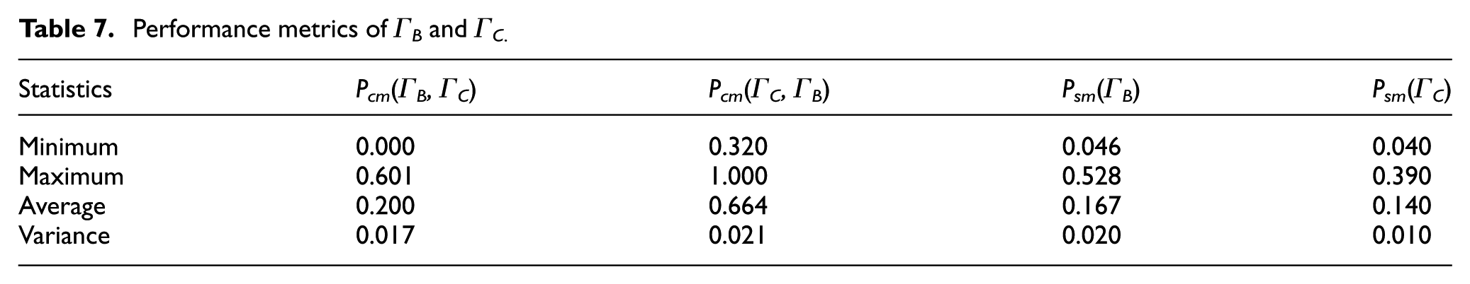
Let ΓB (Γc) denote the obtained Γ of the test using B (C). The performance metrics of the two Pareto frontiers are presented in Table 7. In the table, the minimum, maximum, and average of Pcm(ΓB, ΓC) are smaller than those of Pcm(ΓC, ΓB), respectively. This result indicates that the values of Pcm(ΓB, ΓC) are always smaller than those of Pcm(ΓC, ΓB). The average of Pcm(ΓC, ΓB) is larger than 0.5, whereas that of Pcm(ΓB, ΓC) is smaller than 0.2, which means that more than half of non-dominated solutions in ΓB are dominated by those solutions in ΓC in most cases. For the comparison between the spacing metrics of ΓB and Γc, the results are quite interesting. ΓC outperforms ΓB in the average and maximum values of Psm, while both Pareto frontiers are equal in the minimum value of Psm. It can be inferred from this result that the solutions in ΓC are more evenly distributed than those in ΓB in most cases, and the best extents of spread of both Pareto frontiers are approximate to each other. These situations arise because some operations use machining parameter combinations which own smaller carbon emission and larger machining time without affecting the makespan of a schedule when using C during the optimization procedure. Therefore, it can be concluded that better Pareto frontier can be obtained when C is employed in the considered case instead of B.
Performance metrics of ΓB and ΓC.
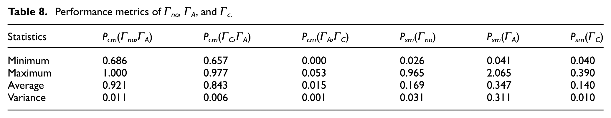
Let Γno denote the obtained Γ of the test using no methods, and ΓA denote the obtained Γ of the test using A. Table 8 reports the performance metrics of Γno, ΓA, and ΓC. The fact that the average of Pcm(Γno, ΓA) is 0.921 shows that about 10% solutions in Γno are not dominated by those in ΓA. Moreover, the minimum, maximum, and average values of Pcm(ΓA, ΓC) are much smaller than those of Pcm(ΓC, ΓA), respectively. This result indicates that the majority of solutions in ΓC are dominated by the solutions in ΓA. Psm(Γno) (Psm(ΓC)) is slightly smaller than Psm(ΓA) (Psm(Γno)). It indicates that C helps to improve the extent of spread in Pareto frontiers since the adoption of C uses the Pareto-optimal combinations instead of all combinations.
Performance metrics of Γno, ΓA, and Γc.
Comparison with the synergistic use of methods
Two tests with both of A and C are employed are generated due to the order of using these methods. Let ΓAC (ΓCA) denote the obtained Γ of the test with A used before (after) C. Figure 5 shows the comparisons of the performance metrics of ΓA, ΓC, ΓAC, and ΓCA. It can be observed from the figure that no solutions in ΓAC are dominated by those in ΓA or ΓC, while almost all of solutions in ΓA and ΓC are dominated by those in ΓAC. Therefore, synergistic improvement on Pareto frontiers can be achieved when both of A and C are employed in the considered case. For the comparisons of the performance metrics of ΓAC and ΓCA, the results are quite interesting. A quite difference is observed between the mean values of Pcm(ΓAC, ΓCA) and Pcm(ΓCA, ΓAC), whereas a slight difference is observed between Psm(ΓAC) and Psm(ΓAC).
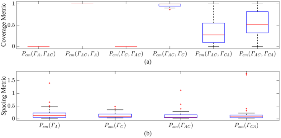
Performance metrics of ΓA, ΓC, ΓAC, and ΓCA.
In order to make the analysis more statistically convincing, two-sample t tests were conducted to determine whether the performance metrics of ΓAC and ΓCA are significantly different from each other. The significance level used in the t tests is 5%, which means that the null hypothesis is rejected if the corresponding p value is smaller than 0.05. The two-sample t test is conducted, and the p values of t test (Pcm(ΓAC, ΓCA), Pcm(ΓCA, ΓAC)) and t test(Psm(ΓAC), Psm(ΓAC)) are 0.008 and 0.461, respectively. The results clearly show that Pcm(ΓAC, ΓCA) and Pcm(ΓCA, ΓAC) are significantly different from each other, while Psm(ΓAC) and Psm(ΓCA) are not. It can be summarized from the above experiments that the order of employing methods affects Pareto frontiers, and better Pareto frontiers can be achieved using A after C in optimization procedures.
Conclusion
This article proposes the mathematical model of a flow shop scheduling problem with variable machining parameters, which considers production efficiency and carbon emission. Two problem-specific scheduling methods (i.e. postponing and improved two-stage optimization methods) are presented and their properties are proved. Then, the steps of employing these methods based on the properties are illustrated. Moreover, a novel D-MOGWO is developed to deal with the problem because of its NP-hard nature. Experiments are designed and conducted to reveal the effectiveness of these methods on improving Pareto frontiers. Three conclusions can be inferred from the computational experiments: (1) the above-mentioned methods significantly help to improve Pareto frontiers, (2) better Pareto frontiers are achieved by the synergistic use of these methods, and (3) the order of using these methods in optimization procedures matters the optimization results.
Future works would include considering other scheduling problems, including job shop scheduling problems, hybrid flow shop scheduling problems, flexible job shop scheduling problems, and so on. Besides, more environmental friendly scheduling methods can be further investigated.
Footnotes
Declaration of conflicting interests
The author(s) declared no potential conflicts of interest with respect to the research, authorship, and/or publication of this article.
Funding
The author(s) disclosed receipt of the following financial support for the research, authorship, and/or publication of this article: This work was supported by the National Natural Science Foundation of China (Nos. 51705263 and 51705262), Natural Science Foundation of Ningbo (No. 2017A610141), and Natural Science Foundation of Zhejiang Province (No. LQ16G010002). This work was also sponsored by K. C. Wong Magna Fund in Ningbo University.