Sage Journals: Discover world-class research

Abstract

Complex ceramic core is the critical part for manufacturing hollow turbine blade in the investment casting process. The complex geometry, small inner structures and high-precision requirements of ceramic cores make them difficult to fabricate, and the shape and dimensional accuracy of ceramic cores are very low in factory practice. To understand the deformation characteristics of ceramic cores, a noisy points recognition algorithm, an extraction method of measuring cross-section contour points and a B-spline iterative fitting algorithm using dominant points of chord deviation are proposed. First, the cross-section contour points were provided through registration, slicing and intersection methods. Second, the noisy points were deleted by convex noisy points and concave noisy points recognition algorithms. Third, the cross-section contour curve of the ceramic core was fitted through B-spline iterative fitting method with chord deviation dominant points. The curves fitted with chord deviation points and curves fitted with local maximum curvature points were compared with simulating data and scanning data, respectively, and the results show that B-spline fitting curve needs fewer chord deviation points than local maximum curvature points, 24.4% fewer in simulation validation and 12.5% fewer in experimental validation. In the end, the bending deformation, torsion deformation and shrinkage deformation errors of ceramic core are established by fitting contour curves of serial cross sections of the ceramic core.

Keywords

Ceramic core B-spline noisy points recognition chord deviation bending deformation torsion deformation shrinkage deformation error

Introduction

Single-crystal hollow turbine blades, which are generally manufactured using near-net-shape investment casting process, are the critical components of high thrust–weight ratio aero-engine. The rejection rate of single-crystal hollow turbine blade is as high as 90%, among which 50% rejections are due to dimension exceeds.¹ One of the most important dimensions of hollow turbine blade is wall thickness, which is determined by the wax pattern contour profile, ceramic core contour profile and the relative location of the wax pattern and ceramic core. In recent years, with the progress of pattern mold optimal design technology^2,3 and ceramic core positioning technology,⁴ the pattern dimension accuracy and ceramic core localization accuracy were well controlled. Thereby, dimensions of the ceramic core become the main constraint to the accuracy of hollow turbine blade wall thickness.

The materials and manufacturing technology of ceramic core are secrets in all countries. China’s ceramic core production technologies lag behind that of developed countries, for the blockade. The common substrate materials of ceramic core are silica and alumina: the silica-based ceramic core is generally used below 1500 °C; when the temperature is higher than 1550 °C, the qualification rate of single-crystal casting blades will fall off; compared with silica-based ceramic core, alumina-based ceramic core has better metallurgical chemical stability and creep resistance, and they can be used at temperature higher than 1550 °C.⁵ Britain and the United States developed high-performance ceramic cores in 1970s, which can be maintained at 1850 °C for 16 h.⁵ Since the 1980s, China has made great progress in the research of alumina-based ceramic cores: AECC Beijing Institute of Aeronautical Materials⁶ has developed the AC-1 and AC-2 alumina-based ceramic core, where AC-1 ceramic core can withstand high temperature up to 1560 °C, the casting success rate is about 70% and the thickness of casting blade is uniform; AC-2 ceramic core performance has been greatly improved compared to AC-1 ceramic core, which has already been used in China’s second-generation single-crystal superalloy investment casting. Chinese Academy of Sciences Institute of Metal Research⁷ has also developed a nano-composite ceramic core, compared to a single component ceramic core, which has better fracture strength, fracture toughness, high-temperature performance, easier to decore. Although the performance of ceramic core materials in China has reached the requirements of casting single-crystal turbine blade, but the dimensional accuracy of the ceramic core is very low. The inspection of ceramic core in industrial production is a problem for its complex structures and less testing standards. As the result, the accuracy of the wall thickness of a turbine blade is difficult to guarantee.

The ceramic core profile is a free-form curve, andB-spline is the most effective mathematical representation of the free-form curve. The B-spline curve fitting is a classic problem of computer aided geometric design (CAGD). It is widely used in many fields such as computational geometry, image processing, machining,^8,9 model reconstruction and pattern recognition. Although the theory of B-spline is mature, knot selection is still difficult to fit B-spline curves and surfaces for two reasons: (1) the number and distribution of optimal knots are difficult to be expressed mathematically. (2) Knot selection is a constrained high-dimensional nonlinear optimization problem. It is difficult to calculate for big number points. B-spline fitting is a least square optimization problem. The earliest algorithm is to transform the constrained optimization problem into an unconstrained optimization problem and then use gradient descent method or Gauss–Newton method¹⁰ to address these problems. However, these algorithms are easy to converge to the local optimal solutions; therefore, these algorithms are also called the local optimization algorithms. In order to surmount the shortcomings of the local optimization algorithm, Beliakov¹¹ proposed a free-knot global optimization algorithm, but the computational efficiency is relatively limited. Some researchers simplify the computational complexity through the iterative process, mainly including adaptive algorithm based on delete point strategy, sparse optimization model and iterative algorithms based on incremental strategy. Yuan et al.¹² proposed an adaptive knot selection algorithm. In this algorithm, the upper bound of knot number is selected through relaxation method based on curvature of discrete points and then the knot displacement was optimized adaptively by reducing the knot number. Kang et al.¹³ described a knot optimization method using a sparse optimization model, a decision index was adopted in his model, and the number and location of knots were optimized by removing insignificant knots and adjusting the positions of the “active” knots. Deng and Lin¹⁴ proposed an iterative algorithm to achieve knot placement optimization by gradually increasing control points or knots. Last decades, evolutionary algorithms have been widely used to solve nonlinear optimization problem, commonly used evolutionary algorithms for solving B-spline knot displacement optimization problem include genetic algorithm and particle swarm optimization method,¹⁵ as well as ant colony algorithm,¹⁶ simulated annealing algorithm¹⁷ and firefly algorithm.¹⁸ Some modified evolutionary algorithms were also researched, such as multi-objective genetic algorithm¹⁹ and global particle swarm optimization (PSO).²⁰ And, some combinatorial evolutionary algorithms such as genetic algorithm + genetic algorithm,²¹ genetic algorithm + PSO²² and random search strategy + genetic algorithm were also researched.²³ Despite the fact that evolutionary algorithms are very powerful, but the computational efficiency of evolutionary algorithms is limited and this is the main reason that hinders their widespread application, moreover, the convergence of evolutionary algorithms cannot be ensured for various kinds of splines. Some scholars study knot optimization in some interesting viewpoints, such as the Bayesian model²⁴ and the Gaussian mixture model;²⁵ knot displacements were optimized through probability distribution. In energy viewpoint, Wang et al.²⁶ established the energy function of B-spline curve through the integral of the weighted sum of squares first derivatives and the second derivatives in the parameter intervals; the knot and control points optimization can gain through energy function minimization; Ravari and Taghirad²⁷ developed a self-adaptive test cluster to identify key knots, based on group test method derived from blood sample test.

It is an effective algorithm by selecting the dominant points^28–30 and then adding points step by step for knot placement optimization; this algorithm is efficient and has good fitting accuracy, but the fitting results are highly dependent on the dominant points: good dominant points can get a smooth B-spline curve with fewer points; poor dominant points will use more points and even cause the fitted curve not smooth enough. Therefore, the selection of dominant points is of great importance. The most commonly used dominant points are endpoints, local maximal curvature (LMC) points, inflection points, turning points, and so on.³¹ These points only consider the curvature information, which is not very good for ceramic core contours fitting, which has multi-segments and various curvatures. In this article, a chord deviation (CD) method is proposed to extract the dominant points, considering both curvatures and distances of the discrete points. The remainder of the current article is organized as follows. In section “Cross-section contour curve of ceramic coreB-spline fitting process,” the whole process of data processing, cross-section contour curve B-spline fitting and deformation decouple for ceramic core are listed. In section “Point data processing,” the point data processing method, including cross-section measurement points extraction method and noisy points recognition method, is studied. In section “B-spline fitting of ceramic core contour curve,” algorithms of computing CD dominant points and B-spline fitting are presented. The simulation and experimental validations are conducted in section “Experiments and discussion.” In section “Deformation of ceramic core,” the bending deformation, torsion deformation and shrinkage deformation of the ceramic core are established through fitting serial sectional contour curves. And the conclusion is given in section “Conclusion.”

Cross-section contour curve of ceramic core B-spline fitting process

In this section, the whole procedure for ceramic core contour curve reconstruction and deformation analysis in this article is briefly listed, shown in Figure 1. Methods and algorithms are detailed in the next two sections. There are seven main steps included as follows:

Collect the point cloud of ceramic core with three-dimensional (3D) measuring devices, such as coordinate measuring machines and laser scanners. In this article, an ATOS optical scanner was used.

Catch the registration of point cloud and computer-aided design (CAD) model of ceramic core with a manual coarse registration and iterative closest point (ICP) fine registration, which can be realized in the commercial software Geomagic Qualify or MeshLab.

Slice up the CAD model and extract the cross-section measuring points.

Data processing. A new denoise algorithm is developed in section “Recognition of noisy points.”

Get the sectional contour points and the bending and torsion deformations of ceramic core cross section using two-dimensional (2D) registration method, same as the method described in step 2.

Extract the dominant points, which cover the characteristics of ceramic core contour. The detailed algorithm is presented in section “B-spline fitting of ceramic core contour curve.”

Create the contour curve of this cross section using B-spline fitting method and calculate the shrinkage deformation errors.

Figure 1.

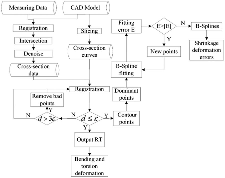
Flowchart of contour curve fitting process for ceramic core.

Point data processing

Cross-section measurement points extraction

Commonly used cross-section measurement points extraction methods are projection and intersection methods. The basis of projection method is using a plane, whose normal vector is perpendicular to the normal vector of point data, to cut off the point cloud; the cross section is obtained by adjusting the distance threshold repeatedly through a static index structure, projecting neighborhood points to the plane and the projection points are treated as cross-section points. The principle of intersection method is based on the intersection of plane and model. The model cross-section data are expressed by the intersection point of the nearest point connection and cross section of point cloud on both sides of the plane. Although the intersection method is more complex than the projection method, but the calculation accuracy is higher, especially the point cloud data of the complex surface, intersection method is used in this article.

Recognition of noisy points

In the process of data collection and data processing of ceramic cores, the noisy points will inevitably be introduced, and the noisy points will affect registration and B-spline fitting accuracy. Noisy points are usually identified by local curvature. The most commonly used local curvature estimation methods are quadratic polynomial scheme and circle scheme. For blade-type curves, the circle scheme is more convenient.³² The discrete curvature is defined as the inverse of the radius of the circles passing through three neighboring points.

Where $P_{i - 1}$ , $P_{i}$ and $P_{i + 1}$ are three adjacent points; $L_{i}$ is the distance between point $P_{i - 1}$ and point $P_{i}$ ; ${L_{i}}^{*}$ is the distance from point $P_{i - 1}$ to point $P_{i + 1}$ ; $Δ S$ is the area of the triangle formed by $P_{i - 1} P_{i} P_{i + 1}$ , as illustrated in Figure 2. The discrete curvature of point $P_{i}$ can be expressed as

K_{i} = 4 Δ S / (L_{i} L_{i + 1} {L_{i}}^{*})

(1)

Figure 2.

Discrete curvature of ordered point set.

The common method to remove noise data points is filtering method, considering discrete curvatures as the digital signals.³³ Because the noise point will affect the curvature of its neighboring points, filters will take the neighboring points as noisy points, which is not always real. Filtering method has better applicability under the condition of numerous and dense measuring points. Jiang et al.³⁴ using the dot product of two vectors from the point to its circle center to recognize noise points. This method can effectively identify the noise points of lines and on the concave side of curves, but cannot identify the noise points on the concave side of curves.

Assuming that $K_{i}$ and $V_{i}$ are the corresponding discrete curvature and center vector, respectively, the following steps can be used to recognize and remove the noisy point:

Remove the significant noisy points directly.

Recognize and remove noisy points on the convex side of the fitting curves. If $K_{i}$ satisfies equation (2), $P_{i}$ is a noisy point. Remove $P_{i}$ from the ordered point set and recalculate $K_{i - 1}$ and $K_{i + 1}$

K_{i} > \frac{a}{3} (K_{i - 1} + K_{i} + K_{i + 1}), a \in [2, 3]

(2)

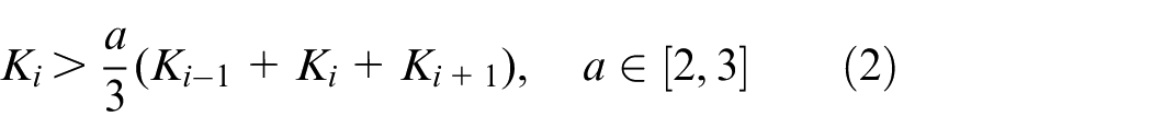
where a reflects the distance of the noisy point away from the fitted curve, choosing a bigger value when the noisy point near the fitting curve and a smaller value when noisy points far from the fitting curve, because that the curvatures of two neighboring points of the noisy point decrease at the first and then increase with the noisy point goes far from the fitted curve.

Recognize and remove noisy points on the concave side of the fitting curves. If $V_{i}$ satisfies equation (3), $P_{i}$ is a noisy point. Remove $P_{i}$ from the ordered point set and recalculate $V_{i - 1}$ and $V_{i + 1}$

{\begin{matrix} dot (V_{i - 1}, V_{i}) < 0 \\ dot (V_{i}, V_{i + 1}) < 0 \end{matrix}

(3)

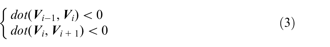
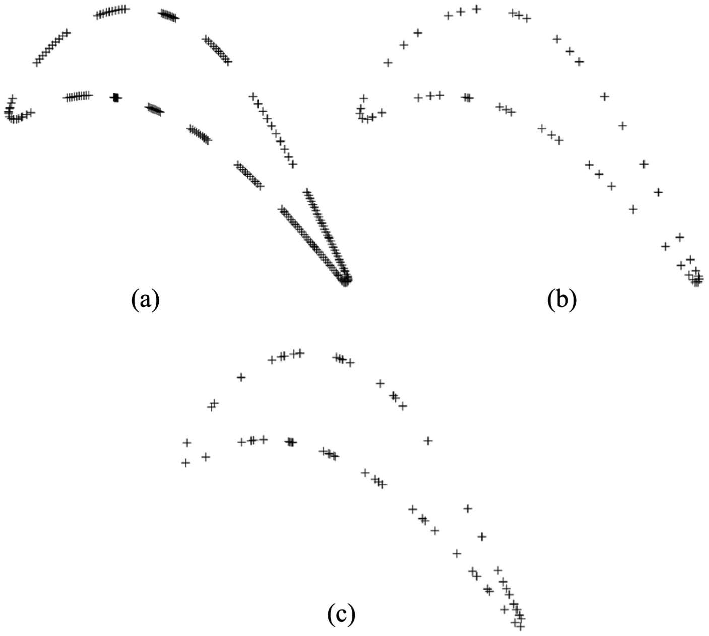
where $dot (,)$ is the dot product of two vectors.

A simple example is used to verify the algorithm and compare with the algorithm in the literature.³² As shown in Figure 3(a), a set of points is sampled on a circle and three noisy points (red dot) are added, and the recognized noisy points (in red circle) of algorithm in the literature³² and algorithm in this article are shown in Figure 3(b) and (c), respectively.

Figure 3.

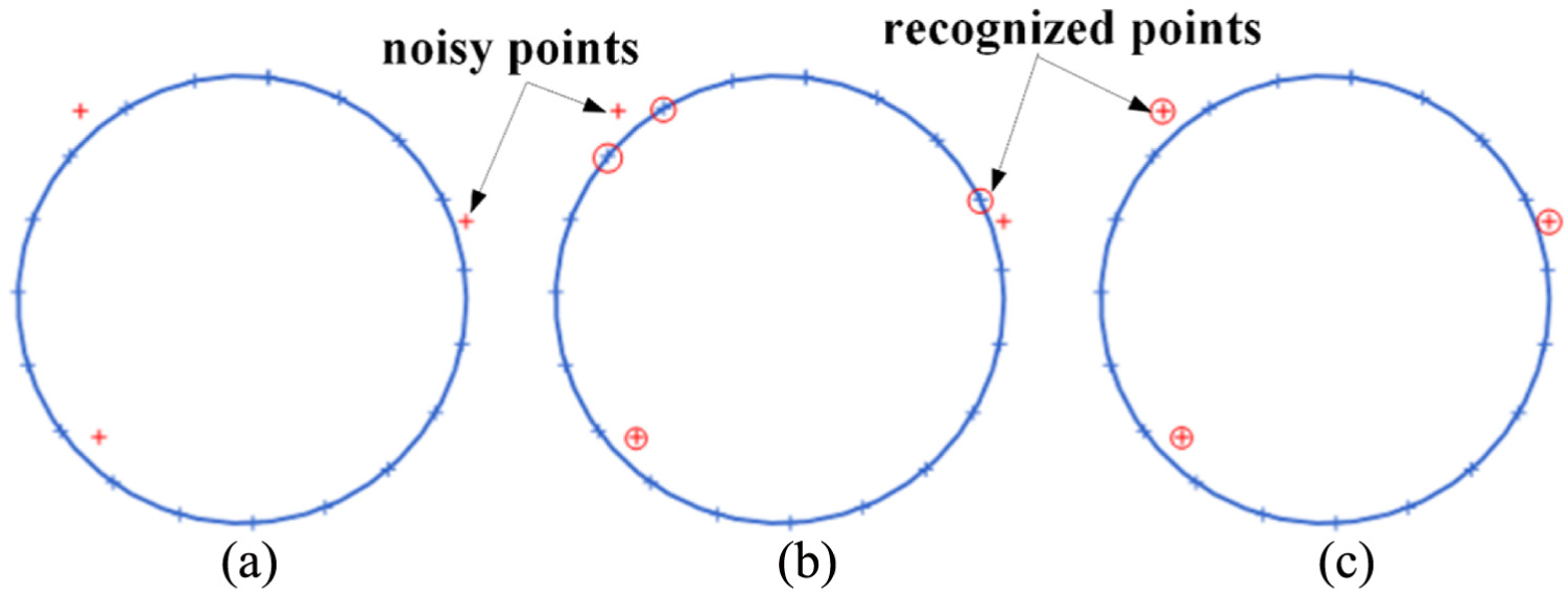
Noisy points recognition: (a) noisy points, (b) result of the literature³² and (c) result of this article.

B-spline fitting of ceramic core contour curve

The kth-order B-spline can be defined as

C (u) = \sum_{i = 0}^{n} B_{i, k} (u) d_{i}

(4)

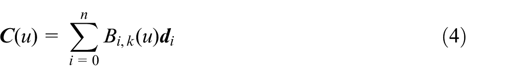
where $B_{i, k} (u)$ is the kth-order B-spline basic function, $D = {d_{i} : i = 0, 1, \dots, n;}$ is the control point, $U = {u_{i} : i = 0, 1, \dots, m + k + 1}$ is the knot vector.

For a point data set $P = {p_{i} : i = 0, 1, \dots, m} (m \geq n)$ , the fitting error of fitted B-spline curve can be expressed as equation (5)

E (d_{0}, d_{1}, \dots, d_{n}) = \frac{1}{m} \sqrt{\sum_{j = 0}^{m} {‖ C (u) - p_{j} ‖}^{2}}

(5)

On the premise of required accuracy, the lesser the points utilized, the smoother the curve can be fitted. The number of points collected by modern digital inspection facilities is very large, and not all points must be used to reconstruct the contour. The smoothness of the fitting curve can be improved using points which reflect the characteristics of the curve, called “dominant points.”²⁸ The dominant points are usually determined by the discrete curvatures of point set. But for ceramic core contour curve which is discontinuous and has various curvatures and curvature sharp changes, dominant points by curvature cannot reflect all the characteristics of the ceramic core contour curve.

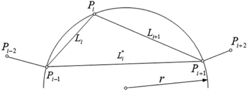
CD is the maximum distance between a curve and one of its chords, illustrated in Figure 4, which can be calculated by equation (6)

δ \approx ρ_{j} - \sqrt{ρ_{j}^{2} - {(L_{j} / 2)}^{2}}

(6)

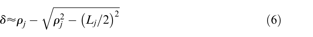
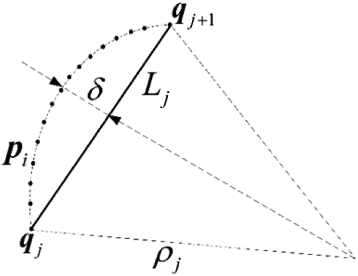
where $ρ_{j}$ is the radius of curvature at point $q_{j}$ , and $L_{j}$ is the distance between $q_{j}$ and $q_{j + 1}$ . According to equation (6), CD is related to both the curvatures and distances of the points.

Figure 4.

Approximation of chord deviation.

Definition 1

CD is the maximum distance of all measured points between two neighboring dominant points to the chord formed by these two dominant points

\hat{δ} = Max {d_{i} : j < i < j + 1}

(7)

In equation (7), $\hat{δ}$ is the estimate CD, $d_{i}$ is the distance of the measurement point $p_{i}$ to the chord of two dominant points $q_{j}$ and $q_{j + 1}$ . When measuring points are dense enough, $\hat{δ} = δ$ . The steps of selecting dominant points according to CD were implemented as below:

Add the two endpoints of each segment of ceramic core cross section to the dominant point set.

Calculate the CD $\hat{δ}$ of two neighboring dominant points and its corresponding measuring point.

If $\hat{δ} > d_{ε}$ , $d_{ε}$ is the given threshold, add the corresponding measuring point to dominant point set.

Repeat steps 2 and 3 until CD of all measurement points is within the threshold.

Having the dominant points, the B-spline can be fitted using the following steps:³⁵

Parameterization: the common parameterization methods include chord length parameterization method and centripetal parameterization method; chord length parameterization method has poor smoothness in the trailing edge of ceramic core, whose curvatures change sharply, so the centripetal parameterization method is used in this article and is expressed in equation (8)

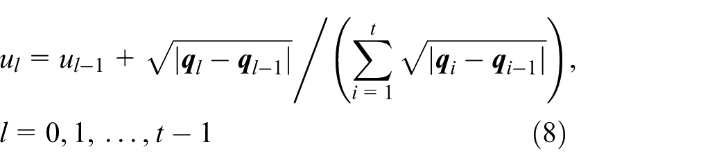
u_{l} = u_{l - 1} + \sqrt{| q_{l} - q_{l - 1} |} / (\sum_{i = 1}^{t} \sqrt{| q_{i} - q_{i - 1} |}), l = 0, 1, \dots, t - 1

(8)

where $Q = [q_{i} : i = 0, 1, \dots, t - 1]$ is the dominant point set, and t is the number of dominant points.

Build the knot vector: the contour of the ceramic core is a periodic closed curve, so $q_{t} = q_{0}$ . $[u_{k}, u_{t + k}]$ can be calculated in parameterization step. $[u_{0}, u_{k - 1}]$ and $[u_{t + k + 1}, u_{t + 2 k}]$ can be determined by the periodicity of the contour curve.

Calculate the control points: get the B-spline basic functions on the knot vector intervals and substitute them in equation (4) and then a group of linear equations are obtained. The control points can be calculated by solving these linear equations.

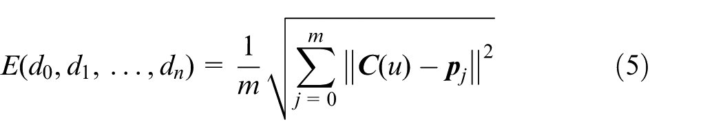
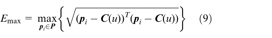
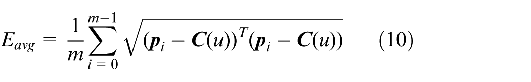
Compute the fitting errors: the B-spline $C (u)$ was got after running steps (a)–(c). The distances from measurement points $P$ to $C (u)$ were taken as the criterion of fitting accuracy. The maximum distance $E_{max}$ and average distance $E_{avg}$ were used in this article

E_{max} = max_{p_{i} \in P} {\sqrt{{(p_{i} - C (u))}^{T} (p_{i} - C (u))}}

(9)

E_{avg} = \frac{1}{m} \sum_{i = 0}^{m - 1} \sqrt{{(p_{i} - C (u))}^{T} (p_{i} - C (u))}

(10)

Selection of new dominant points: calculate the distances of each measuring point between two neighboring dominant points, and add the point having the maximal distance to dominant point set if the maximal distance is bigger than permitting error.

Repeat steps (a)–(e) until all the measuring points are within the permitting distance.

Only one new point can be added between two neighboring dominant points in each iteration. Using the above B-spline fitting algorithm, the actual contour curve and designed contour curve are obtained. We can get the corresponding couples of points by sampling the actual contour curve and design contour curve using uniform parameter sampling strategy and know the shrinkage deformation errors of this cross section of the ceramic core through computing the distances between these corresponding points.

Experiments and discussion

In this section, two experiments of B-spline fitting ceramic core contour curves, with both CD points and LMC points, were implemented and compared.

Validation with CAD data

40 points were sampled uniformly on trailing edge segment of designed ceramic core contour, and 10 points were sampled uniformly on each remaining segments, and totally 150 points are shown in Figure 5(a). These 150 sampled points were exactly on the CAD curve with no error. And, these 150 sampled points were taken as candidate points to fit B-spline curve. With the criterion of CD $d = 0.2 mm$ , 51 dominant points can be obtained, showed in Figure 5(b). 59 dominant points including endpoints and local curvature maximum points generated through extreme curvature method are shown in Figure 5(c). Comparing Figure 5(b) and (c), using CD method, there are more dominant points on the leading edge and trailing edge of the ceramic core.

Figure 5.

Dominant points of ceramic core contour: (a) CAD contour sampled points, (b) chord deviation dominant points and(c) LMC points.

According to the process of B-spline fitting in section “B-spline fitting of ceramic core contour curve,” the maximum fitting error $E_{max} = 0.01 mm$ was taken as the stopping criteria, the B-spline fitting results of the CD dominant points are shown in Table 1 and the result of LMC points is shown in Table 2.

Table 1.

Fitting errors of chord deviation dominant points for CAD data.

Iterations	Number of points	Maximal fitting error (mm)	Average fitting error (mm)
0	51	0.018436	0.002665
1	56	0.017156	0.002216
2	61	0.014793	0.001697
3	63	0.014198	0.001416
4	64	0.013652	0.001407
5	65	0.008705	0.001328

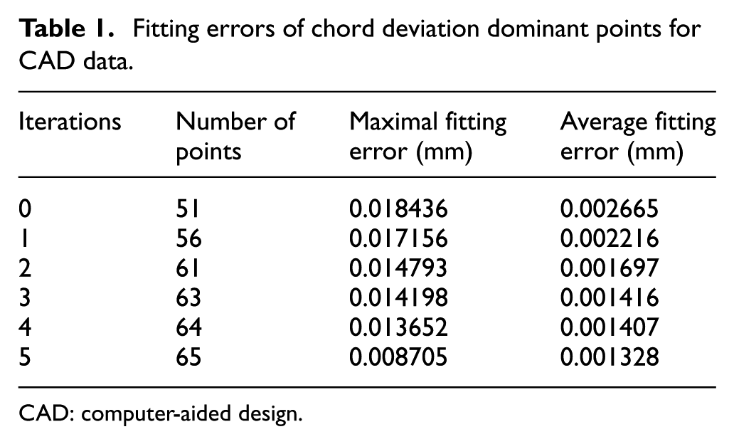
CAD: computer-aided design.

Table 2.

Fitting errors of LMC points for CAD data.

Iterations	Number of points	Maximal fitting error (mm)	Average fitting error (mm)
0	59	0.147861	0.005817
1	66	0.082279	0.005295
2	76	0.025541	0.001706
3	83	0.019320	0.001065
4	85	0.013722	0.001072
5	86	0.007985	0.000882

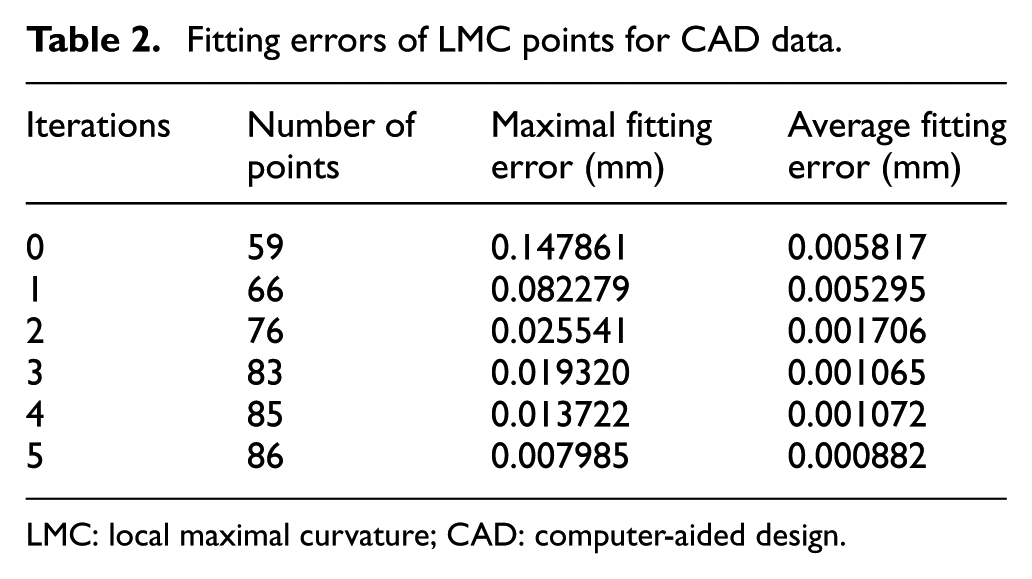
LMC: local maximal curvature; CAD: computer-aided design.

Comparing Tables 1 and 2, using CD dominant points at iteration 0, the maximal fitting error is 0.018436 mm and the average fitting error is 0.002665 mm; using LMC points at iteration 0, the maximal fitting error is 0.147861 mm and the average fitting error is 0.005817 mm. When the stopping criteria reached, the number of CD dominant points needed for fitting ceramic core contour is 65, compared to 86 LMC points, which is reduced by 24.4%. The initial fitted contour curve of ceramic core is shown in Figure 6.

Figure 6.

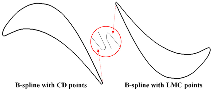
Comparison of fitted ceramic core contour.

Form Figure 6, we can see that the B-spline using CD dominant points is more accurate than B-spline using LMC points, especially at the trailing edge.

Validation with experiment data

In this section, some experiment results are given to verify the effectiveness the proposed method. The ceramic core is shown in Figure 7(b), its measurement points shown in Figure 7(c) are collected using an ATOS Core Optical 3D Scanner (shown in Figure 7(a)) of GOM company in China and the limit measurement accuracy of this ATOS is 0.015 mm.

Figure 7.

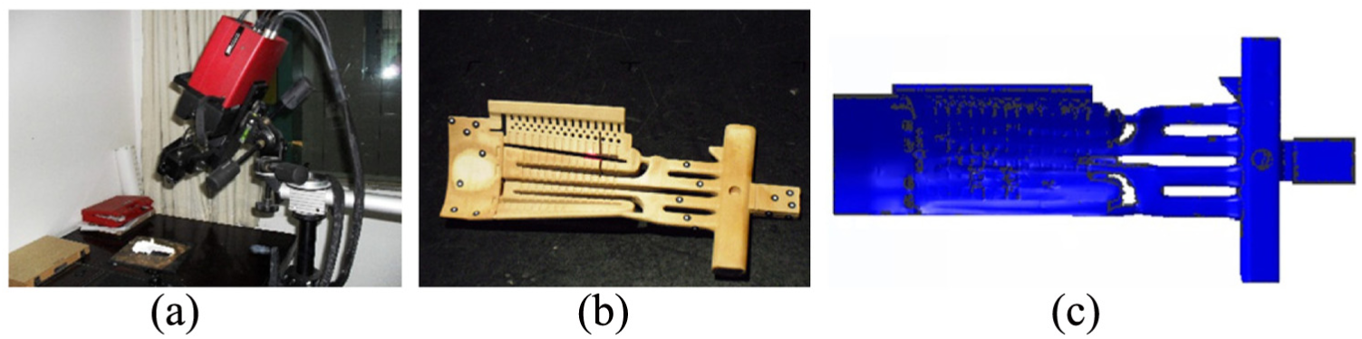
Measurement experiment of ceramic core: (a) ATOS scanner, (b) ceramic core and (c) measuring data.

The common method for point data set segmentation is segmenting points according to the similarity of the discrete normal vectors, but this method is not suitable for sintered ceramic cores for the irregular fillets. CAD model–guided segmentation method can effectively segment of the point data set of the blades.³⁶ So, this method is employed in this article. The designed ceramic core cross section is shown in Figure 8(b), in which the solid line is the contour of the designed cross section of the ceramic core. The cross-section measurement points are shown in Figure 8(a). The extraction process of measurement points of ceramic core contour is available in Figure 1. After the 2D registration of the cross-section measurement points and designed contour lines, if the nearest point of a measurement point falls on one of the designed contour lines, this point is a measured contour point; otherwise, it is an internal point. The extraction result is shown in Figure 8(c).

Figure 8.

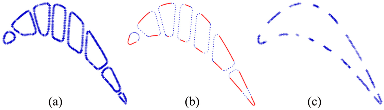
Extract contour measured points of ceramic core: (a) measuring points, (b) designed contour and (c) extraction result.

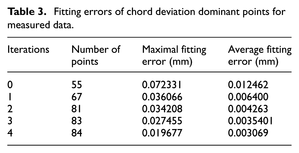
Then, the CD method and extreme curvature method were used to extract dominant points and fit the B-spline, and the results are shown in Tables 3 and 4, respectively.

Table 3.

Fitting errors of chord deviation dominant points for measured data.

Iterations	Number of points	Maximal fitting error (mm)	Average fitting error (mm)
0	55	0.072331	0.012462
1	67	0.036066	0.006400
2	81	0.034208	0.004263
3	83	0.027455	0.0035401
4	84	0.019677	0.003069

Table 4.

Fitting errors of LMC points for measured data.

Iterations	Number of points	Maximal fitting error (mm)	Average fitting error (mm)
0	51	0.226470	0.017149
1	74	0.077115	0.007956
2	86	0.031174	0.003859
3	92	0.030534	0.003462
4	96	0.018082	0.002539

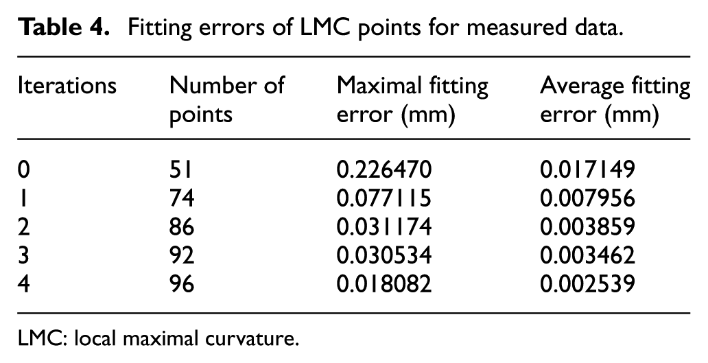
LMC: local maximal curvature.

Due to the influence of manufacturing errors, measurement errors, measurement data fusion errors and surface roughness,³⁷ even after the noisy point processing, the fluctuation of measurement point data is inevitable. Take the maximum fitting error $E_{max} = 0.02 mm$ as the stopping criteria, then the number of points needed for fitting ceramic core contour using CD method is 84, 12.5% less than that of the LMC method. In iteration 0, the maximum fitting error of CD method is 0.072331 mm, 68.06% less than that of LMC method, the average fitting error of CD method is 0.0125 mm, 26.9% less than that of LMC method. The initial fitted contour of the ceramic core is shown in Figure 9, in which the solid black lines are the designed contour of the ceramic core.

Figure 9.

Comparison of fitted contour of measurement points.

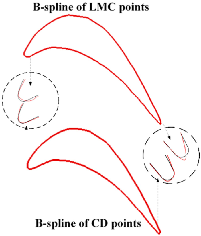
B-spline using CD dominant points are more accurate than B-spline using extreme curvature dominant points, especially in the leading and trailing edges.

Deformation of ceramic core

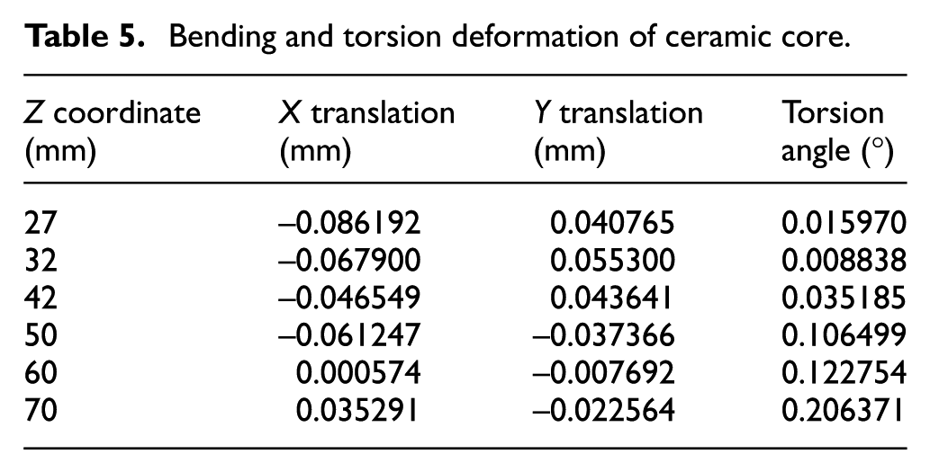
In this section, the bending deformations, torsion deformations and shrinkage errors of this measured ceramic core are calculated. A group of parallel cross sections was obtained by slicing the measurement data of ceramic core. The bending and torsion deformation of each cross section were calculated by the translation vector $T$ and the rotation matrix $R$ obtained from the 2D registration

T = [T_{x}, T_{y}] R = [\begin{matrix} \cos θ & - \sin θ \\ \sin θ & \cos θ \end{matrix}]

(11)

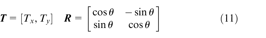
where $T_{x}$ is the bending deformation in the X direction, $T_{y}$ is the bending deformation in the Y direction, and $θ$ is the torsion angle. The bending and torsion deformation results are presented in Table 5.

Table 5.

Bending and torsion deformation of ceramic core.

Z coordinate (mm)	X translation (mm)	Y translation (mm)	Torsion angle (°)
27	−0.086192	0.040765	0.015970
32	−0.067900	0.055300	0.008838
42	−0.046549	0.043641	0.035185
50	−0.061247	−0.037366	0.106499
60	0.000574	−0.007692	0.122754
70	0.035291	−0.022564	0.206371

250 points were uniformly sampled on the designed sectional contour curves and the inspected sectional contour curves of the ceramic core. The trailing edge points were taken as the starting points and sampled points were ordered anticlockwise. The signed distance d of the corresponding points are on the measurement sectional contour curves and the designed sectional contour curves, where d is positive when the measurement point is outside the designed sectional contour curve and negative when the measurement point is in the designed sectional contour curve. The signed distance d is the shrinkage deformation error of the ceramic core at this point. The shrinkage deformation errors of the sectional curve were gained by quadratic interpolation of the signed distance of 250 couples of corresponding points. The shrinkage deformation errors of section Z =32 mm and section Z =60 mm are shown in Figure 10, in which I—the trailing edge, II—the pressure side, III—the leading edge and IV—the suction side.

Figure 10.

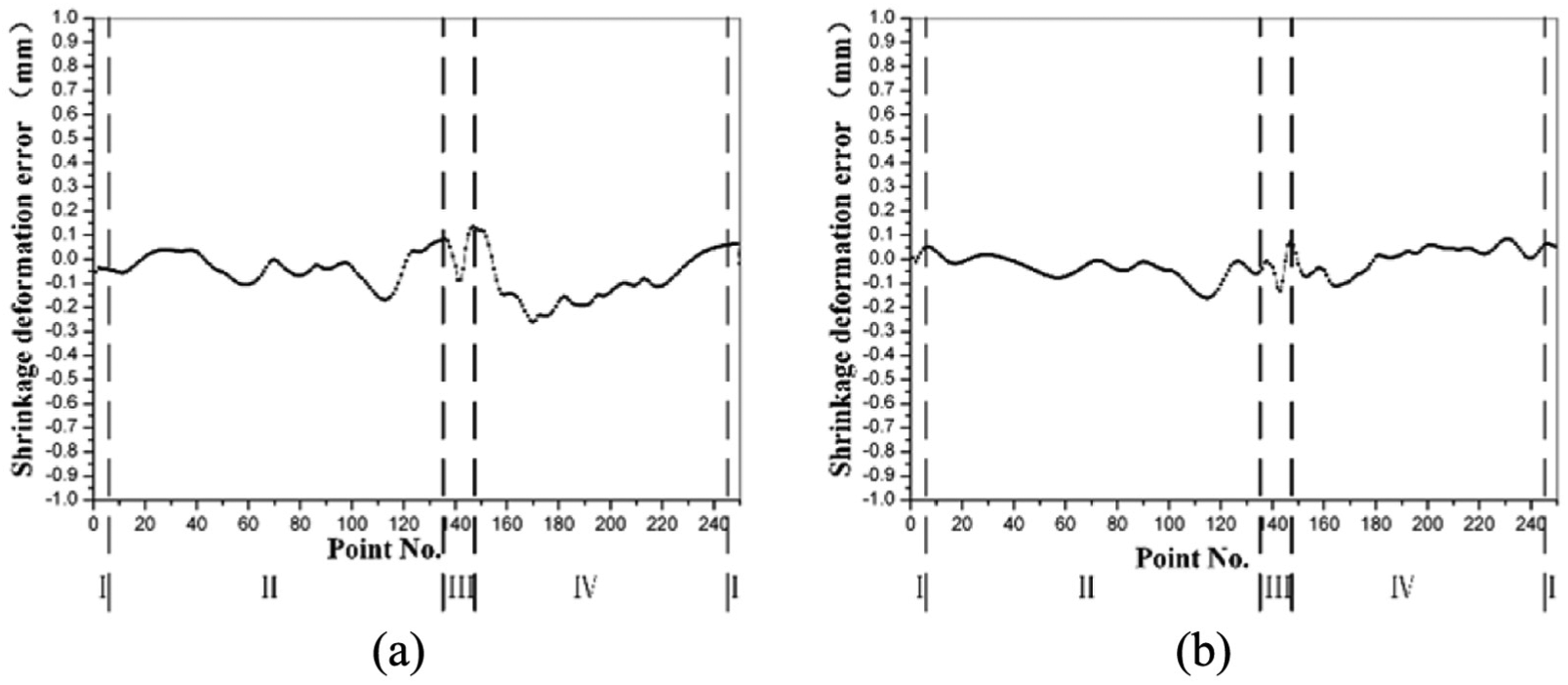
Shrinkage deformation errors of ceramic core: (a) section Z =32 mm and (b) section Z =60 mm.

The model of the ceramic core was reconstructed through lofting method with all the fitted contour curves. The reconstructed model is shown in Figure 11. The deformation nephogram by comparing the measurement points to the design model is shown in Figure 12. The deformation nephogram by comparing the reconstructed model to the design model is shown in Figure 13.

Figure 11.

Reconstructed model of ceramic core.

Figure 12.

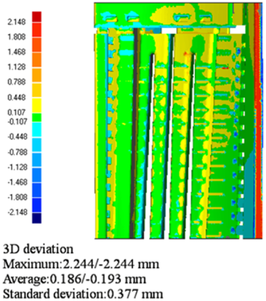
Deformation results of measurement points.

Figure 13.

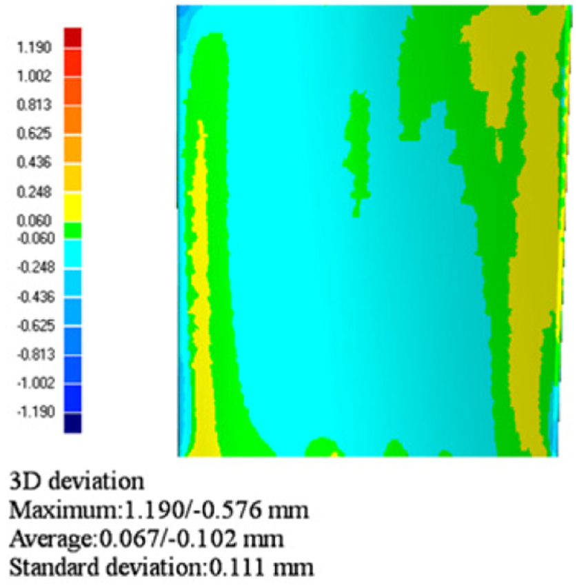
Deformation results of the reconstructed model.

From Figure 12, we can see that the deformation of the exhaust edge, pin-fin holes and some fillets is much larger than the deformation of the other structures of the ceramic core. The dimensions of exhaust edge, pin-fin holes and fillets have very little influence on the thickness of casting blade, so the deformation of them is not research priority of this article. Through fitting the contour curve, the deformation of the profile of the ceramic can be directly researched, not affected by its inner structures. Meanwhile, the shrinkage deformation error, essential to reverse design of the die of ceramic core, needs the contour curves. The ceramic core has shrinkage deformation toward the pressure surface according to Figure 13.

Conclusion

An algorithm of measurement data points processing and an algorithm of B-spline contour curve approximation have been outlined in this article for segmental and noisy data points of the ceramic core. The following conclusions can be drawn by comparing these two algorithms to others in recent literature:

Noisy points can be identified and removed effectively by classifying them into convex noisy points and concave noisy points. First, identify and remove the convex noisy points and then identify and remove the concave noisy points.

Using CD dominant points, the number of points needed for ceramic core B-spline contour curve fitting is reduced by 24.4% and 12.5% in simulation and experiment, respectively, compared to traditional LMC points. CD dominant points reflect the shape of ceramic core cross section better than LMC points, especially at the leading edge and trailing edge positions.

The whole process of ceramic core deformation analysis proposed in this article has a good guiding function for the deformation calculation and analysis of ceramic cores and blades, and it can provide references for researchers and engineers.

Footnotes

Declaration of conflicting interests

The author(s) declared no potential conflicts of interest with respect to the research, authorship and/or publication of this article.

Funding

The author(s) disclosed receipt of the following financial support for the research, authorship, and/or publication of this article: This work was supported by the National Natural Science Foundation of China (No. 51371152).

ORCID iD

Xiandong Zhang

References

Qiu

Song

J-H

et al . Dimensional control of nickel-based single crystal turbine blade investment casting by process control optimization. Int J Metalca St 2018; 12(3): 469–479.

Jiang

R-S

Zhang

D-H

et al . A deformation compensation method for wax pattern die of turbine blade. Int J Adv Manuf Tech 2017; 88: 3195–3203.

Dong

Zhang

et al . Geometric parameter-based optimization of the die profile for the investment casting of aerofoil-shaped turbine blades. Int J Adv Manuf Tech 2011; 57: 1245.

Jiang

R-S

Wang

W-H

Zhang

D-H

et al . Wall thickness monitoring method for wax pattern of hollow turbine blade. Int J Adv Manuf Tech 2016; 83: 949–960.

Shifeng

Dinghua

Kun

Research progress in precise shape-controlling technology of single crystal hollow turbine blades. Rare Metal Mat Eng 2012; 41: 559–564.

Dou

Yan

. Reversing design methodology of ceramic core for hollow turbine blade based on measured data. In: ASME 2014 international mechanical engineering congress and exposition, Montreal, QC, Canada, 14–20 November 2014, pp.V02AT02A051–V002AT002A051. New York: American Society of Mechanical Engineers.

Qin

Zhang

et al . Alumina-based ceramic core nano-composites for investment casting. Rare Metal Mat Eng 2007; 36: 774–776.

Huang

Zhang

et al . Tool path generation for ultra-precision polishing of freeform optical surfaces in an off-axis three-mirror imaging system. Proc IMechE, Part B: J Engineering Manufacture 2017; 231: 814–824.

Huang

Zhu

LM.

Feedrate scheduling for interpolation of parametric tool path using the sine series representation of jerk profile. Proc IMechE, Part B: J Engineering Manufacture 2017; 231: 2359–2371.

10.

Lim

Haron

Surface reconstruction techniques: a review. Artif Intell Rev 2014; 42: 59–78.

11.

Beliakov

Least squares splines with free knots: global optimization approach. Appl Math Comput 2004; 149: 783–798.

12.

Yuan

Chen

Zhou

Adaptive B-spline knot selection using multi-resolution basis set. IEE Trans 2013; 45: 1263–1277.

13.

Kang

Chen

et al . Knot calculation for spline fitting via sparse optimization. Comput Aided Design 2015; 58: 179–188.

14.

Deng

Lin

Progressive and iterative approximation for least squares B-spline curve and surface fitting. Comput Aided Design 2014; 47: 32–44.

15.

Pottmann

Leopoldseder

Hofer

et al . Industrial geometry: recent advances and applications in CAD. Comput Aided Design 2005; 37: 751–766.

16.

Y-Y

L-X

Wen

Q-Y

et al . Data fitting via chaotic ant swarm. In: Jiao

Wang

Gao

et al . (eds) International conference on natural computation. Berlin: Springer, 2006, pp.180–183.

17.

Aganj

Keriven

Pons

J-P.

Photo-consistent surface reconstruction from noisy point clouds. In: 16th IEEE international conference on image processing (ICIP), Cairo, Egypt, 7–10 November 2009, pp.505–508. New York: IEEE.

18.

Gálvez

Iglesias

Firefly algorithm for explicit B-spline curve fitting to data points. Math Probl Eng 2013; 2013: 528215.

19.

Valenzuela

Delgado-Marquez

Pasadas

Evolutionary computation for optimal knots allocation in smoothing splines. Appl Math Model 2013; 37: 5851–5863.

20.

Gálvez

Iglesias

Particle swarm optimization for non-uniform rational B-spline surface reconstruction from clouds of 3D data points. Inform Sciences 2012; 192: 174–192.

21.

Gálvez

Iglesias

Puig-Pey

Iterative two-step genetic-algorithm-based method for efficient polynomial B-spline surface reconstruction. Inform Sciences 2012; 182: 56–76.

22.

Gálvez

Iglesias

A new iterative mutually coupled hybrid GA-PSO approach for curve fitting in manufacturing. Appl Soft Comput 2013; 13: 1491–1504.

23.

Spiriti

Eubank

Smith

et al . Knot selection for least-squares and penalized splines. J Stat Comput Sim 2013; 83: 1020–1036.

24.

Mamic

Bennamoun

Automatic Bayesian knot placement for spline fitting. In: Proceedings of the international conference on IEEE image processing, Thessaloniki, 7–10 October 2001, pp.169–172. New York: IEEE.

25.

Zhao

Zhang

Yang

et al . Adaptive knot placement using a GMM-based continuous optimization algorithm in B-spline curve approximation. Comput Aided Design 2011; 43: 598–604.

26.

Wang

W-K

Zhang

Park

et al . Reducing control points in lofted B-spline surface interpolation using common knot vector determination. Comput Aided Design 2008; 40: 999–1008.

27.

Ravari

Taghirad

HD.

Reconstruction of B-spline curves and surfaces by adaptive group testing. Comput Aided Design 2016; 74: 32–44.

28.

Park

Lee

J-H.

B-spline curve fitting based on adaptive curve refinement using dominant points. Comput Aided Design 2007; 39: 439–451.

29.

Park

B-spline surface fitting based on adaptive knot placement using dominant columns. Comput Aided Design 2011; 43: 258–264.

30.

Zhao

Zhu

et al . Look-ahead interpolation of short line segments using B-spline curve fitting of dominant points. Proc IMechE, Part B: J Engineering Manufacture 2015; 229: 1131–1143.

31.

Razdan

Knot placement for B-spline curve approximation. Tempe, AZ: Arizona State University, 1999.

32.

Dong

Zhao

et al . Modeling of shrinkage during investment casting of thin-walled hollow turbine blades. J Mater Process Tech 2017; 244: 190–203.

33.

Zhao

et al . Adaptive knot placement in B-spline curve approximation. Comput Aided Design 2005; 37: 791–797.

34.

Jiang

Ben-chi

Lian

et al . A B-spline curve fitting algorithm based on contour key points. Appl Math Mech 2015; 36: 423–431.

35.

Bu-Qing

Ding-Yuan

Computational geometry: curve and surface modeling. Oxford: Elsevier, 2014.

36.

Cheng

Zhang

et al . Model registration control point set selection for turbine blade shape inspection. J Mech Eng 2009; 45: 240–246.

37.

Singh

Pandey

PM.

Fabrication and characterization of open cell porous regular interconnected metallic structure with solid core. Proc IMechE, Part B: J Engineering Manufacture 2018; 232: 305–316.

B-spline contour curve approximation and deformation analysis of complex ceramic core

Abstract

Keywords

Introduction

Cross-section contour curve of ceramic core B-spline fitting process

Point data processing

Cross-section measurement points extraction

Recognition of noisy points

B-spline fitting of ceramic core contour curve

Definition 1

Experiments and discussion

Validation with CAD data

Validation with experiment data

Deformation of ceramic core

Conclusion

Footnotes

Declaration of conflicting interests

Funding

ORCID iD

References